Velocity Structure in the Orion Nebula. I. Spectral Mapping in Low-Ionization Lines

Abstract

High-dispersion echelle spectroscopy in optical forbidden lines of O⁰, S⁺, and S²⁺ is used to construct velocity-resolved images and electron density maps of the inner region of the Orion nebula with a resolution of $10~{}\mathrm{km\ s}^{-1}{}\times 3\arcsec\times 2\arcsec$. Among the objects and regions revealed in this study are (1) the Diffuse Blue Layer: an extended layer of moderately blue-shifted, low-density, low-ionization emission in the southeast region of the nebula; (2) the Red Bay: a region to the east of the Trapezium where the usual correlation between velocity and ionization potential is very weak, and where the emitting layer is very thick; and (3) HH 873: a new redshifted jet to the southwest of the Trapezium.

Note: A version of this paper with full-resolution figures can be obtained from http://www.ifront.org/wiki/Spectral_Mapping_Paper_I

1. Introduction

The Orion Nebula is the prime example of a blister-type $\mathrm{H\,\scriptstyle II}$ region (Israel, 1978), in which ultraviolet radiation from the high-mass Trapezium stars heats and ionizes the front surface of the molecular cloud OMC-1, giving rise to a “champagne flow” of ionized gas (Tenorio-Tagle, 1979; Yorke, 1986; Henney et al., 2005) away from the cloud. Although the basic empirical model was proposed more than 30 years ago (Zuckerman, 1973), the nebula continues to present theoretical challenges due to the extraordinarily rich phenomenology that is continually uncovered by advances in observational techniques (see O’Dell, 2001, and references therein). The Orion Nebula presents one of the best opportunities available for studying in detail the star formation process in high density environments. A rich cluster of more than a thousand low-mass stars is associated with the nebula and centered on the Trapezium (Hillenbrand, 1997). There is evidence that the star formation rate has accelerated over the past few million years (Hillenbrand & Hartmann, 1998), with the youngest stars concentrated towards the center of the cluster. Indirect evidence from the survival of the proplyds in the core of the nebula (Henney & O’Dell, 1999) indicates that the highest mass stars are probably even younger ($10^{4}$–$10^{5}$ years). Dense molecular gas is primarily concentrated in a north-south oriented lane (Johnstone & Bally, 1999), displaced $\simeq 30\arcsec$ to the west of the Trapezium, containing embedded sites at which star formation is still ongoing (Smith et al., 2004). A thorough understanding of the structure and dynamics of the $\mathrm{H\,\scriptstyle II}$ region is necessary in order to understand the role of the high-mass stars in limiting the star formation process by dispersing the molecular cloud and in evaporating circumstellar material around young low-mass stars (Hester & Desch, 2005).

Previous global studies of the nebula have been mainly based on imaging in emission line filters (Hester et al., 1991; Pogge et al., 1992) or spectrophotometry (Baldwin et al., 1991; Esteban et al., 1998), and therefore only give an average over different emitting regions along the line of sight. High-resolution spectroscopic studies show a wealth of detail with many ions showing complex multi-component kinematic profiles (Campbell & Moore, 1918; Wilson et al., 1959; Deharveng, 1973; Goudis et al., 1984; Hanel, 1987; Castañeda & O’Dell, 1987; Jones, 1992; O’Dell & Wen, 1992; Meaburn et al., 1993; Massey & Meaburn, 1993; O’Dell et al., 1993; Wen & O’Dell, 1993; Massey & Meaburn, 1995; O’Dell et al., 2001). Although in principle high resolution optical spectroscopy can allow the disentanglement of different emission regions, in practice progress has been slow due both to the complex nature of the object and the incomplete nature of the data-sets available. Global spatio-spectral studies of the nebula have generally been carried out with Fabry-Perot instruments (O’Dell et al., 1997a; Rosado et al., 2001; de La Fuente et al., 2003), the velocity resolution of which ($>30~{}\mathrm{km\ s}^{-1}{}$) is not sufficient to study any but the highest velocity flows in the nebula. Radio recombination line studies (e.g., Wilson et al., 1997) offer the possibility of higher spectral resolution but have been confined to hydrogen lines, where the thermal Doppler broadening of $\simeq 20~{}\mathrm{km\ s}^{-1}$ largely negates this advantage. On the other-hand, most multi-line high-resolution ($\sim 5~{}\mathrm{km\ s}^{-1}{}$) echelle spectroscopy (Henney & O’Dell, 1999) has only covered restricted areas of the nebula. A notable exception is the recent study by Doi et al. (2004, hereafter DOH04), which covered the entire inner region of the nebula in the [$\mathrm{N\,\scriptstyle II}$], H$\alpha$ and [$\mathrm{O\,\scriptstyle III}$] lines with a resolution of $2\arcsec\times 1.5\arcsec\times 8$ km s^-1. In this paper, we present a study in the lines of [$\mathrm{S\,\scriptstyle II}$]$\lambda$6716,6731, [$\mathrm{O\,\scriptstyle I}$]$\lambda$6300, [$\mathrm{S\,\scriptstyle III}$]$\lambda$6312, which is complementary to the DOH04 study. Whereas DOH04 concentrated on the high-velocity emission from jets and HH objects, this paper emphasizes the more subtle variations in the bulk of the nebular gas, which typically moves at transsonic velocities of 5–20 km s^-1.

The four lines that we study cover a range of ionization stages from low to moderate ionization. These correspond to different spatial zones as a result of the ionization stratification that is typically found in ionized nebulae. The [$\mathrm{O\,\scriptstyle I}$] line is emitted principally by the partially ionized gas in the ionization front, whereas the [$\mathrm{S\,\scriptstyle III}$] line is emitted only by ionized gas in the interior of the nebula, where hydrogen is fully ionized, although excluding the most highly ionized interior of the nebula, where sulfur is triply ionized. The emission of the [$\mathrm{S\,\scriptstyle II}$] lines contains contributions from both the fully ionized and partially ionized zones and furthermore the difference in critical density of the two lines of the doublet allows the determination of the electron density. Our set of lines is of generally lower ionization than that studied in DOH04 since the [$\mathrm{S\,\scriptstyle II}$] and [$\mathrm{O\,\scriptstyle I}$] lines extend to more neutral regions than does [$\mathrm{N\,\scriptstyle II}$], whereas [$\mathrm{S\,\scriptstyle III}$] is weak from the most highly ionized regions, which emit strongly in [$\mathrm{O\,\scriptstyle III}$]. Previous, low spectral resolution studies of the electron density in the Orion nebula using these lines have suffered from the problem that the derived densities are merely an average of the conditions in different regions of the nebula, weighted by the [$\mathrm{S\,\scriptstyle II}$] emissivity. However, by kinematically resolving the different components of the line, we are able for the first time to separately determine the electron density in different zones of the nebula.

Some preliminary results from this study have already been presented in Henney et al. (2005), where the patterns of global kinematics in the nebula were compared with the results of hydrodynamical simulations of champagne flows. The current paper contains a much fuller description of our dataset and an empirical analysis of the complex structure of the spatio-kinematic maps, concentrating on velocities within $\pm 30~{}\mathrm{km\ s}^{-1}{}$ of the systemic velocity and presenting evidence for the existence of many new nebular features. Our results on the low-velocity HH 528 outflow are reported in a separate paper (Henney et al., 2006), whereas another companion paper (Henney & García-Díaz, 2006, referred to hereafter as Paper II) will present a more detailed study of some of the new features we have identified in the nebula, including comparison with high-resolution HST imaging.

In § 2 we describe our observations and the data reduction steps that we followed in order to produce flux- and velocity-calibrated spectra and velocity channel maps of emission and electron density. In § 3 we use these results to empirically derive the physical conditions and kinematics of different features in the nebula, many of which have not been previously discussed in the literature.

2. The Observations and Data Reduction

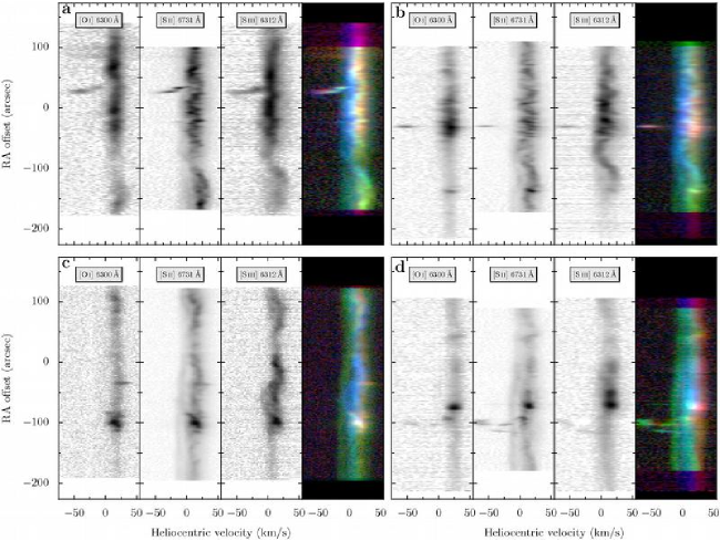
Figure 1.— Sample two-dimensional slit spectra of [$\mathrm{O\,\scriptstyle I}$] 6300 Å, [$\mathrm{S\,\scriptstyle II}$] 6731 Å, and [$\mathrm{S\,\scriptstyle III}$] 6312 Å for four representative slit positions. All spatial offsets are measured with respect to $\theta^{1}$Ori C: (a) $68.8\arcsec$ W, (b) $22.2\arcsec$ W, (c) $40.4\arcsec$ E, and (d) $88.4\arcsec$ E. The grayscale negative images are each scaled to the maximum intensity in each slit and use a “square root” transfer function, which emphasizes fainter features. The color, positive-scaled images are composites of the three emission lines for each slit, with [$\mathrm{O\,\scriptstyle I}$] represented by red, [$\mathrm{S\,\scriptstyle II}$] by green, and [$\mathrm{S\,\scriptstyle III}$] by blue.

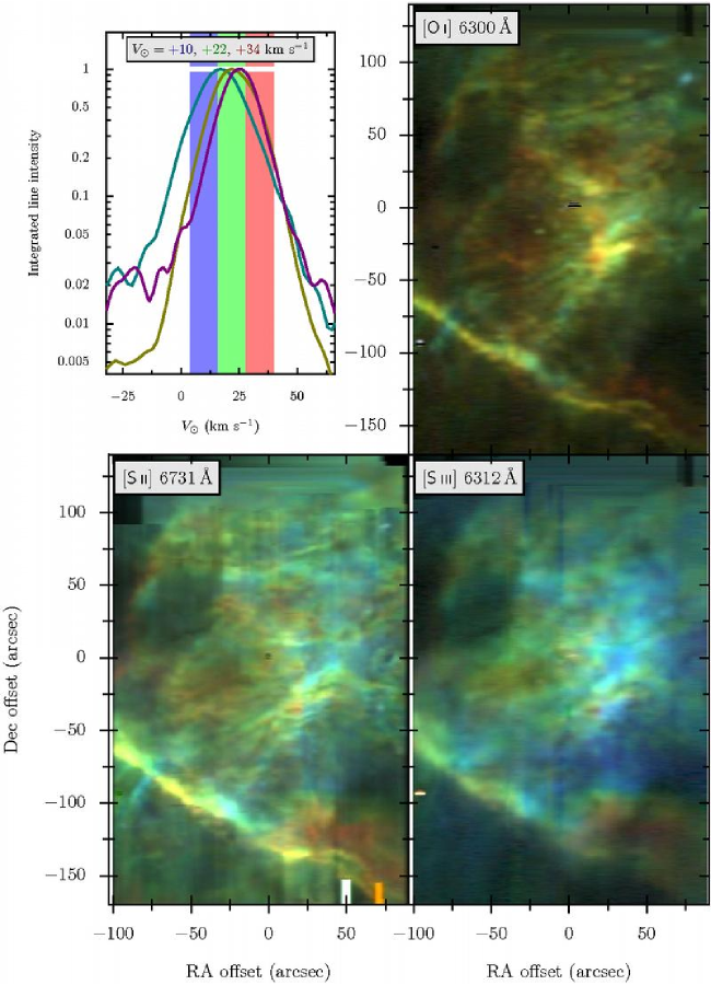
Figure 2.— Natural-weighted channel maps of the line cores, color-coded as shown in the top-left panel, showing the coarse velocity changes within $\pm 18~{}\mathrm{km\ s}^{-1}$ of the peak [$\mathrm{S\,\scriptstyle II}$] velocity of $V_{\odot}=+22~{}\mathrm{km\ s}^{-1}$. For each emission line, an identical intensity scale is used for each of the three RGB channels, allowing meaningful comparison to be made between the colors in the different maps. The upper-left panel indicates the position of each velocity channel on the integrated spectrum of the entire nebula (logarithmic scale) in the three lines. Left to right: [$\mathrm{S\,\scriptstyle III}$] (turquoise), [$\mathrm{S\,\scriptstyle II}$] (gold), [$\mathrm{O\,\scriptstyle I}$] (purple).

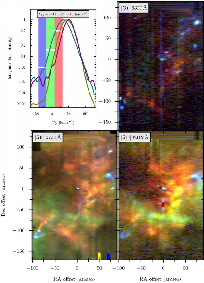
Figure 3.— Same as Fig. 2 but for the blue side of the line profiles, corresponding to heliocentric velocities between $V_{\odot}=-20~{}\mathrm{km\ s}^{-1}$ and $+16~{}\mathrm{km\ s}^{-1}$. Since the emission line profiles are falling towards the blue in this velocity range, different normalizations are used for the images in the 3 velocity bands, as indicated by the horizontal white lines in the top-left panel.

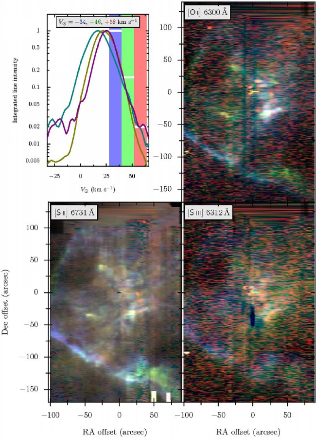
Figure 4.— Same as Fig. 2 but for the red side of the line profiles, corresponding to heliocentric velocities between $V_{\odot}=+28~{}\mathrm{km\ s}^{-1}$ and $+64~{}\mathrm{km\ s}^{-1}$. Since the emission line profiles are falling towards the red in this velocity range, different normalizations are used for the images in the 3 velocity bands, as indicated by the horizontal white lines in the top-left panel.

High-resolution spectroscopic observations of the Orion Nebula were obtained from two different observatories: one set from Kitt Peak National Observatory (KPNO), and the other set from Observatorio Astronómico Nacional at San Pedro Mártir, B.C., Mexico (SPM). The first set of spectra was obtained with the echelle spectrograph mounted on the 4 m telescope at KPNO and is described in detail in O’Dell et al. (2001) and DOH04. The $300\times 0.8^{\prime\prime}$ slit was oriented north-south on the nebula and exposures were taken at a grid of different declinations (separation $\approx 2^{\prime\prime}$). This dataset, with velocity resolution of 8 $\mathrm{km\ s}^{-1}$, consists of 37 positions for [$\mathrm{S\,\scriptstyle II}$]$\lambda\lambda$6716,6731 Å lines in two disjoint regions of the nebula: one in the East, centered on $\mathrm{RA}=05^{\mathrm{h}}35^{\mathrm{m}}21\fs 5$, and one in the West, centered on $\mathrm{RA}=05^{\mathrm{h}}35^{\mathrm{m}}11\fs 70$.

The SPM observations were obtained in 2002 October and 2003 January for [$\mathrm{S\,\scriptstyle II}$] (55 pointings) and in December 2003 for the [$\mathrm{O\,\scriptstyle I}$] and [$\mathrm{S\,\scriptstyle III}$] lines (60 pointings) using the MES-SPM instrument (Manchester Echelle Spectrometer, Meaburn et al., 2003) attached to the 2.1 m telescope in its f/7.5 configuration. For the majority of the exposures, we used a 150$\mu$m ($\equiv$ 2 arcsec) slit, giving a velocity resolution (FWHM) of 12 $\mathrm{km\ s}^{-1}$, while for some exposures we used a 70$\mu$m ($\equiv$ 0.95 arcsec) slit, giving a velocity resolution of 6 $\mathrm{km\ s}^{-1}$. The $312\arcsec$-long slit was oriented North-South for most of the observations, except for one EW-oriented exposure in each line at a position $9.6\arcsec$ south of $\theta^{1}$Ori C. We used the star JW499 ($\alpha=05^{\mathrm{h}}35^{\mathrm{m}}15\fs 89$, $\delta=-05\arcdeg 23\arcmin 49\farcs 92$; Jones & Walker, 1988) as a reference point for all of our pointings. For each position we took two spectral exposures with duration of 450 s for the 150 $\mu$m slit (with $2\times 2$ pixel on-chip binning), or 900 s for the 70 $\mu$m slit (with no on-chip binning). Thorium-Argon lamp spectra were taken for wavelength calibration between each slit position. In order to establish the exact position of the slit in each pointing we took direct “slit images” of short duration, in which the diffraction grating was replaced by a mirror, with the slit removed for half of the duration of the exposure. This was necessary since the telescope pointing proved insufficiently reliable to guarantee $2\arcsec$ offsets between exposures.

Combining the datasets from the two observatories gives 92 NS pointings in the [$\mathrm{S\,\scriptstyle II}$] doublet, spanning an interval of 190.6^′′ in RA. For the [$\mathrm{O\,\scriptstyle I}$] and [$\mathrm{S\,\scriptstyle III}$] lines, which were observed simultaneously due to their proximity in wavelength, we have only the 60 NS pointings from SPM, spanning a similar interval in RA.

The initial stages of data reduction (bias removal, flat fielding, cosmic ray removal) were carried out using standard IRAF tasks. This was followed by rectification and first-order wavelength calibration of the two-dimensional spectra based on the comparison lamp spectra, also using standard IRAF tasks.

After transforming all the spectra to a common heliocentric velocity frame, we carried out a series of further steps in order to produce internally consistent, well-calibrated velocity cubes in each of the four emission lines. These were implemented using purpose-written Fortran and Python routines.

1. Continuum emission was removed by fitting a quadratic function to each row of each two-dimensional spectrum, including only line-free regions in the fit.

2. An astrometric solution was found for each of the “slit images” mentioned above, using several of the Trapezium cluster stars. This allowed us to accurately determine the slit position of each exposure.

3. Due to variations in atmospheric transparency between exposures, it was necessary to perform a slit-to-slit relative intensity calibration. This was done by comparison with the spectrum from the horizontal slit position.

4. In the same way, the relative slit-to-slit wavelength calibration was refined using the horizontal slit spectrum. The line centroid velocity as a function of position was calculated for each slit and small shifts were introduced in the velocity scale to force agreement with the horizontal slit at the point where they crossed. The shifts required were typically less than 2 $\mathrm{km\ s}^{-1}$.

5. For the [$\mathrm{O\,\scriptstyle I}$] line it was necessary to remove the night-sky component, which occurs at 0 $\mathrm{km\ s}^{-1}$ in the geocentric frame. We had chosen the dates of the observations such that the heliocentric correction means that this component is not blended with the main emission from the nebula. Since the profile of this component was seen to be constant along the length of the slit, it was straightforward to remove by fitting an analytic profile to the summed spectrum of each slit (a hyper-Gaussian profile was used). The centroid of the fitted profile provided an additional check on the accuracy of the wavelength calibration for this line.

Examples of the resultant two-dimensional spectra after following all these steps are shown in Figure 1. Only the longer wavelength component of the [$\mathrm{S\,\scriptstyle II}$] doublet is shown. In this and all following figures, heliocentric velocities, $V_{\odot}$, are used and positions are specified as arcsecond offsets ($x$, $y$) with respect to the principal ionizing star of the nebula, $\theta^{1}$Ori C, which has J2000 coordinates $\alpha=05\ 35\ 16.46$, $\delta=-05\ 23\ 23.2$ (Høg et al., 2000). Transformations between these offsets and the commonly used coordinate-based naming scheme of O’Dell & Wen (1992) are given in the Appendix.

The preceding steps have not significantly degraded the spatial or velocity resolution of the original data. However, in order to combine the individual slit spectra into a three-dimensional data cube, it is necessary to degrade the resolution to that of the lowest common denominator. To that end, we carried out the following steps:

1. The instrumental linewidths were homogenized by smoothing the SPM 70 $\mu$m spectra by 10 $\mathrm{km\ s}^{-1}$ and the KPNO spectra by 9 $\mathrm{km\ s}^{-1}$ to give the same instrumental width as for the SPM 150 $\mu$m spectra (12 $\mathrm{km\ s}^{-1}$ FWHM).

2. The slit spectra were binned/interpolated onto a uniform grid in RA, declination, and heliocentric velocity, with voxel size of $0.6\arcsec{}\times 0.6\arcsec{}\times 4~{}\mathrm{km\ s}^{-1}{}$, in order to produce the three-dimensional data cube. During this stage, we also applied a “de-jittering” procedure to each two-dimensional iso-velocity cut in order to eliminate unsightly striping due to residual inter-slit variations. For each velocity value, a mean intensity of extended diffuse emission was calculated for each slit, and these were then filtered across the slits by a 5-point smoothing kernel to produce a correction to the intensity of each slit.

The resulting data cubes for the lines of the three ions are shown in Figures 2 to 4 as velocity channel maps. Each of the images encodes the emission in three adjacent 12 $\mathrm{km\ s}^{-1}$ velocity channels as blue, green, and red, respectively, moving from more negative to more positive velocities, as shown on the logarithmically scaled line profile of the final panel. We estimate the spatial resolution of the resulting images to be $3\arcsec\times 2\arcsec$ for [$\mathrm{S\,\scriptstyle II}$] and $4\arcsec\times 2\arcsec$ for [$\mathrm{O\,\scriptstyle I}$] and [$\mathrm{S\,\scriptstyle III}$]. Despite our best efforts, some artefacts remain from the combination of different datasets. These are identifiable as bright or dark vertical stripes on the images, which are more prominent in the line wings, where the intrinsic signal is weaker. They are chiefly caused by imperfections in the rectification and continuum removal, or in some cases due to reflections caused by a bright star falling in the slit (particularly at an RA offset of $0$).

Further steps were necessary in order to photometrically calibrate our data. We used spectrophotometric observations from the literature in order to “pin down” the absolute line fluxes at different points of the nebula by comparing with the velocity-integrated intensity that we observe at the same point. For [$\mathrm{O\,\scriptstyle I}$] and [$\mathrm{S\,\scriptstyle III}$], we used the observations of Baldwin et al. (1991), who give the absolute flux of the blend of these two lines, together with the higher spectral resolution observations of Baldwin et al. (2000), who give the ratio of the two lines. In both cases the observations are for an EW slit, positioned to the W of $\theta^{1}$Ori C, which overlaps with our own data over a length of $\simeq 40\arcsec$. Note that, although we obtain the [$\mathrm{O\,\scriptstyle I}$] and [$\mathrm{S\,\scriptstyle III}$] lines in the same spectrum, we still need to externally calibrate their ratio because of the unknown variation in the spectrograph efficiency over the wavelength range of the two lines. Since we performed all the observations with the same spectrograph settings, we have assumed that the relative efficiency is the same for all slits, and, indeed, comparison with the Baldwin et al. data confirms this assumption.

For the [$\mathrm{S\,\scriptstyle II}$] doublet, a greater variety of spectrophotometric data exists in the literature (Baldwin et al., 1991; Pogge et al., 1992; Esteban et al., 1998). However, in this case, we have the added complication that our data are a combination of results from two different instruments at two different observatories. Hence the calibrations of the SPM-MES and KPNO slits were performed separately. The density-sensitive ratio of the two [$\mathrm{S\,\scriptstyle II}$] lines is of key importance, so we took particular care to verify our velocity-integrated results against those of previous authors.

We have also calculated channel maps of electron density and of the line ratios [$\mathrm{O\,\scriptstyle I}$]/[$\mathrm{S\,\scriptstyle II}$] and [$\mathrm{S\,\scriptstyle III}$]/[$\mathrm{S\,\scriptstyle II}$], which are shown in Figure 5 and 6. In both cases, the sum of the two [$\mathrm{S\,\scriptstyle II}$] lines was used in the denominator and for the ratios with [$\mathrm{O\,\scriptstyle I}$] and [$\mathrm{S\,\scriptstyle III}$] the [$\mathrm{S\,\scriptstyle II}$] maps were first smoothed slightly in order to better match the spatial resolutions.

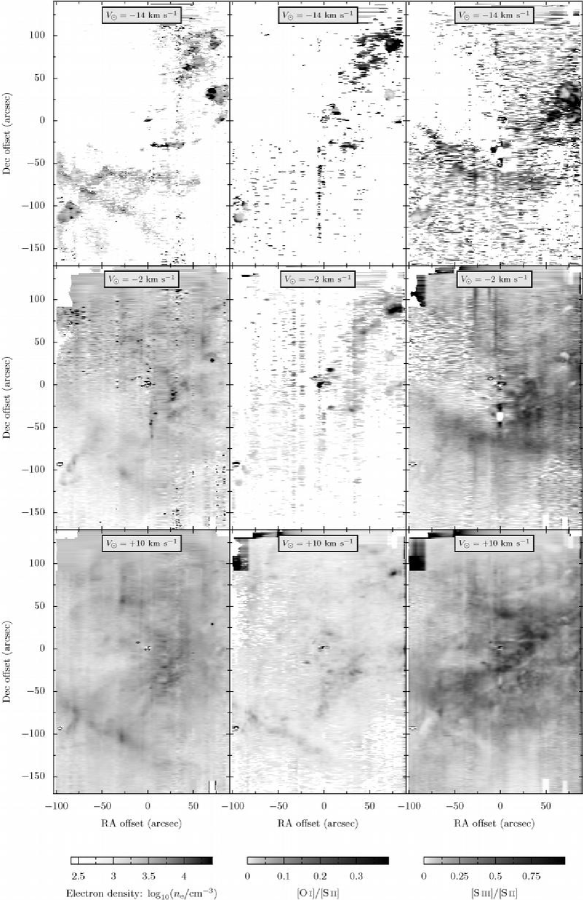
Figure 5.— Blueshifted isovelocity channel maps of [$\mathrm{S\,\scriptstyle II}$]-derived electron density (logarithmic negative grayscale), [$\mathrm{O\,\scriptstyle I}$]/[$\mathrm{S\,\scriptstyle II}$] ratio, and [$\mathrm{S\,\scriptstyle III}$]/[$\mathrm{S\,\scriptstyle II}$] ratio (linear negative grayscales). Each velocity channel is of width 12 $\mathrm{km\ s}^{-1}$.

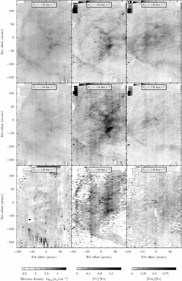
Figure 6.— Same as Figure 5 but for redshifted velocities.

3. Kinematic-ionization structure of the nebula

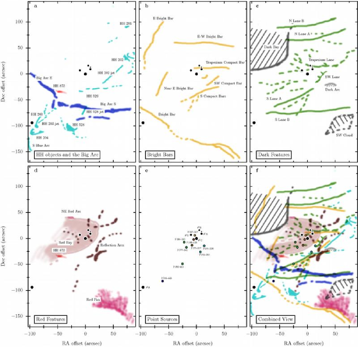
Figure 7.— Finding charts for features in our channel maps. (a) Blueshifted features assosciated with the Big Arc (dark blue) and HH outflows (light blue), together with the newly identified redshifted jet (red). (b) Bright Bars and newly identified compact bars (yellow). (c) Dark regions corresponding to low-ionization lanes (olive green), foreground extinction features (mid gray), and the dark arc (light gray). (d) Redshifted features seen in higher-ionization lines (light pink) and lower-ionization lines (magenta), together with reflection filaments seen in the far-red (brown). (e) OB stars (filled black circles) and proplyds (open circles). The shading of the proplyds indicates their peak [$\mathrm{O\,\scriptstyle I}$] velocity from 20 $\mathrm{km\ s}^{-1}$ (blue) to 31 $\mathrm{km\ s}^{-1}$ (red). (f) Superposition of all the features.

In this section we provide an empirical description of the nebular structure and kinematics as revealed by our spectra. We begin with a general overview of the kinematics and follow with more detailed treatments of some of the individual objects and spectral features, both those that are already known and those that are described for the first time in this paper. We have made use of both the isovelocity channel maps and the position-velocity spectra when identifying features. The channel maps are most useful for taking advantage of the image-processing capacity of the human brain in order to reveal large-scale, spatially coherent features that are not readily apparent in the individual slit spectra. However, it is always necessary to return to the original position-velocity spectra, which in many cases are of higher spectral resolution, in order to confirm identifications and make precise measurements. Figure 7 illustrates in cartoon form the location of all the features discussed below.

When naming new objects, we have tried to follow the established conventions of the literature and to employ names that evoke only the two-dimensional appearance of the feature on the plane of the sky. By deliberately avoiding descriptions that presuppose a certain model of the three-dimensional structure of the nebula, we hope to avoid the problem of the names becoming obsolete with advances in our physical understanding. Some widely used examples of the existing nomenclature are rays—narrow, precisely linear features, which may be bright or dark, usually aligned with some source of illumination; bars—bright, approximately linear features; lanes—dark, approximately linear features; arcs—curved, more or less elongated features, which may be dark or bright.

3.1. Large-scale nebular properties

3.1.1 The line core

The general structure of the emission near the systemic velocity of the three lines is shown in the 3-color isovelocity images of Figure 2. Note that the centroid velocity of the molecular gas behind the nebula is around $V_{\odot}=+28~{}\mathrm{km\ s}^{-1}{}$, lying between the green and the red channels of this figure. The emission is very clumpy and filamentary in [$\mathrm{O\,\scriptstyle I}$], rather less so in [$\mathrm{S\,\scriptstyle II}$], and much smoother and more diffuse in [$\mathrm{S\,\scriptstyle III}$]. The principal features of the nebula are well known—see Goudis (1982) for a compilation of early work on the subject.

1. The region of peak nebula brightness, lying just to the southwest of the Trapezium, centered around ($25$, $-25$). This is a region of highly inhomogeneous brightness, especially in the lower ionization lines, with much structure that is only poorly resolved in our observations, but that can be appreciated in HST images.

2. The Bright Bar (e.g., Elliott & Meaburn (1974)), a prominent low-ionization, approximately linear emission feature to the southeast, running from ($-100$, $-60$) to ($90$, $-170$). This is the ionized portion of the famous Orion Bar (Werner et al., 1976), which is a concentration of dense molecular gas, offset to the southeast from the ionized emission. The region south of the Bright Bar is brighter in [$\mathrm{S\,\scriptstyle II}$] than in either of the other lines.

3. The Dark Bay, a foreground extinction feature, which can be appreciated as a general reduction in brightness to the northeast, with a southern border running from ($-100$, $0$) to ($-30$, $20$).

As one passes from [$\mathrm{O\,\scriptstyle I}$], through [$\mathrm{S\,\scriptstyle II}$], to [$\mathrm{S\,\scriptstyle III}$], the line core becomes more weighted towards the blue overall, as can be appreciated both from the integrated line profiles (shown in the top-left panel of the figure) and from the general hue of each image. However, this trend is not universal across the face of the nebula and two broad regions of redshifted emission are present in the [$\mathrm{S\,\scriptstyle III}$] map (shown in fig. 7d. The first of these lies to the east of the Trapezium, and we name this region the Red Bay since its general shape seems to mimic that of the Dark Bay that lies to the northeast of it. It is discussed further in § 3.4 below. The second region lies just north of the western end of the Bright Bar, and we name it the Red Fan due to its appearance in low ionization lines as a set of bright plumes that fan away from that portion of the Bright Bar.

There is considerable agreement in the pattern of velocity changes between the three different lines. In each case, the most blueshifted gas is found in a broad C-shaped arc to the north, west, and south of the Trapezium, which wraps around the Red Bay. Apart from the two redshifted regions mentioned above, reduced blueshifts are also seen in the Bright Bar and in various other large-scale filamentary structures that criss-cross the nebula. In addition to the bright bars that have previously been reported in the literature (O’Dell & Yusef-Zadeh, 2000), we have identified several examples of more compact bars towards the core of the nebula, which are labelled in Figure 7b. Furthermore, we have also detected a series of dark lanes, which are labelled in Figure 7c. Owing to the narrowness of most of these features, a full investigation of their nature requires a detailed comparison with high-resolution HST imaging, which is beyond the scope of the current paper, but is carried out in Paper II.

3.1.2 The blue flank

Figure 3 shows further isovelocity images, but this time for the blueshifted flank of the emission lines. There is an overlap with Figure 2 in the sense that the red channel of Figure 3 is the same as the blue channel of Figure 2. All of the lines are falling away sharply towards negative velocities in this velocity range, so that, if a naturally weighted brightness scale (as in Fig. 2) had been used, then all the images would be dominated by the red channel. Instead, different scales are used for the 3 channels (with maxima as indicated by white horizontal lines in the top-left panel) so as to give a more balanced color scheme. As a result, care must be taken in interpreting the images since the brightest blue features are 10 times fainter than the brightest red features.

The [$\mathrm{O\,\scriptstyle I}$] line is generally very faint in these velocity channels, and concentrated in very localized regions. In the most negative (blue) channel, one sees only emission from high-velocity Herbig-Haro shocks: HH 201 to the northwest, HH 202 to the west, HH 269/507 to the southwest and HH 203/204 to the southeast. In the least negative (red) channel, one sees both low-velocity Herbig-Haro objects, such as HH 528 to the south, and the blue wings of the bright bars.

In the [$\mathrm{S\,\scriptstyle II}$] and [$\mathrm{S\,\scriptstyle III}$] lines, the most negative channel is again dominated by the HH objects, but the other two channels show much more extensive emission. In particular, the green channel, centered around $V_{\odot}=-2~{}\mathrm{km\ s}^{-1}$ is very prominent in the south of the nebula in these two lines. Part of this emission is due to the Big Arc (O’Dell et al., 1997a; Doi et al., 2004), a broad, elongated swathe of intermediate velocity blueshifted emission, running from southwest from ($-100$, $0$) to ($-50$, $-60$) and then more nearly west to ($80$, $-75$) (see Fig. 7a). Although it is visible in [$\mathrm{S\,\scriptstyle II}$] (faintly) and [$\mathrm{S\,\scriptstyle III}$], the Big Arc is most prominent in higher ionization lines, such as [$\mathrm{O\,\scriptstyle III}$], and it is discussed in greater detail in Paper II. In addition to the Big Arc, widespread diffuse emission is seen in this velocity channel, being especially strong in [$\mathrm{S\,\scriptstyle II}$]. The [$\mathrm{S\,\scriptstyle II}$] density sensitive line ratio map (Fig. 5) show this emission to come from low-density gas, which we refer to as the Southeast Diffuse Blue Layer and which is discussed further in § 3.6 below.

3.1.3 The red flank

Figure 4 shows isovelocity images for the redshifted flank of the emission lines, with the blue channel here being identical to the red channel of Figure 2. Again, unequally weighted brightness scales have been used to compensate for the general fall-off in the line profiles away from their core. This time, the brightest red features are a factor of 50 times fainter than the brightest blue features.

Even with this help, for [$\mathrm{O\,\scriptstyle I}$] very little emission can be discerned above the noise in the redmost channel ($V_{\odot}=+52$ to $+64~{}\mathrm{km\ s}^{-1}$), except for a faint glow in the extreme northwest. In the [$\mathrm{S\,\scriptstyle II}$] and [$\mathrm{S\,\scriptstyle III}$] images, on the other hand, faint but extensive emission is found, concentrated towards the region southwest of the Trapezium. In the [$\mathrm{S\,\scriptstyle II}$] image, which has a significantly higher signal-to-noise than the other two, the emission can be seen to be concentrated into clumps and arcs (see Fig. 7d), which usually do not coincide with the bright filaments seen at bluer velocities. We believe that this emission arises from the scattering of nebular emission lines by dust particles that lie behind the nebula. See further discussion below in § 3.5.

Most of the jets and outflows in the Orion Nebula show only blueshifted emission (see Henney et al., 2006), but we have detected a hitherto unreported redshifted jet in our data, which is clearly visible in the [$\mathrm{O\,\scriptstyle I}$] and [$\mathrm{S\,\scriptstyle II}$] images of Figure 4 at a position of ($-40$, $-35$). This is described in detail in § 3.2.2 below.

At the more moderate redshift of the blue and green channels ($V_{\odot}=+28$ to $+52~{}\mathrm{km\ s}^{-1}$), one sees mainly the red wings of the flows from the bright bars (see Paper II).

3.2. Herbig-Haro outflows

The classical M42 Herbig-Haro objects HH 201–204 and accompanying jets (O’Dell et al., 1997b) are all present in our spectra, together with more recently recognised outflows such as HH 529 (see Fig. 3). Although these flows do appear in the velocity channels that we are considering, the majority of their emission is at higher blueshifted velocities (see, for example, Fig. 1d, which shows the HH 203 jet and the HH 203/204 bowshocks). We therefore defer detailed discussion of these objects to a later paper and merely note their presence here.

Other Herbig-Haro flows do not show such high velocities and the entirety of their emission is contained within the velocity range considered in this paper. These include the large, low velocity HH 528 flow and two objects that are described here for the first time: HH 873, a newly discovered redshifted jet, and the South Blue Arc, which may represent a leading bowshock of the HH 203/204 system.

3.2.1 HH 528

HH 528 is a large-scale, low-ionization, low-velocity outflow in the core of the Orion Nebula (O’Dell & Bally, 1999; Bally et al., 2000). Although it is one of the largest outflows in the nebula, its existence was recognized only relatively recently, owing both to its lack of high-velocity emission and the fact that its bowshock, despite being very large and bright, is superimposed on the low-ionization emission from the Bright Bar. Previous spectroscopic studies have been unable to kinematically resolve the outflow from the systemic nebular emission. The multi-line velocity mapping that we present here allows the emission from the outflow and its bowshock to be cleanly separated for the first time from the more redshifted nebular gas, showing it to be blueshifted by $10\pm 3~{}\mathrm{km\ s}^{-1}$ with respect to the systemic velocity of the molecular cloud. Further details of our radial velocity measurements of this object are given in a separate paper (Henney et al., 2006).

3.2.2 HH 873

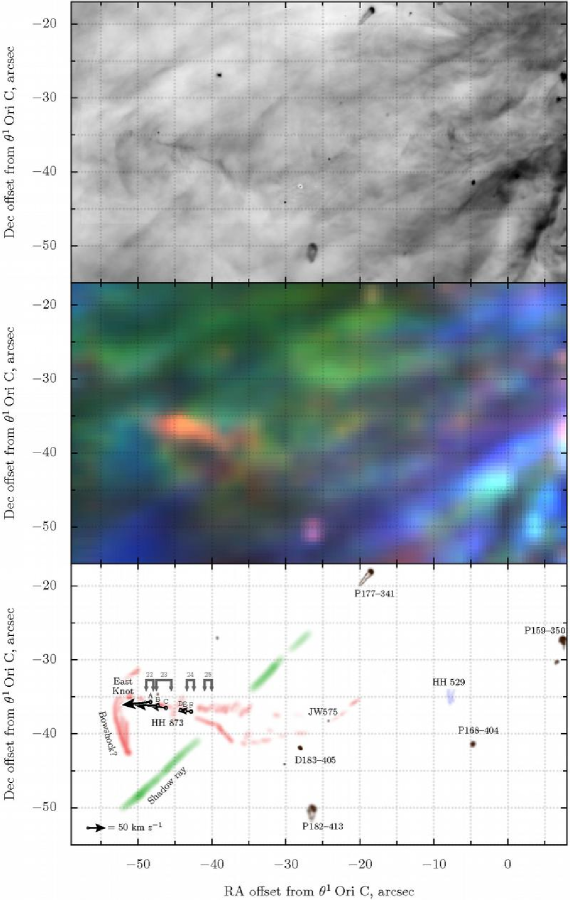
Figure 8.— Observations of the HH 873 redshifted jet. Top: Portion of the HST WFPC2 image in the [$\mathrm{N\,\scriptstyle II}$] line. Center: Three-channel color-coded [$\mathrm{N\,\scriptstyle II}$] velocity map from ground-based observations, with $12~{}\mathrm{km\ s}^{-1}$ wide channels centered on $V_{\odot}=42$ (red), $30$ (green), and $18$ (blue) $\mathrm{km\ s}^{-1}$. Bottom: Finding chart for objects of interest in the image. Also shown are proper motions of individual knots (A–F) in the HH 873 jet and the positions of the slits (22–25) used to extract radial velocities.

This newly detected redsfifted jet is shown in greater detail in Figure 8. The top panel shows an HST WFPC2 image of the region in the [$\mathrm{N\,\scriptstyle II}$] line (f658n filter) at a resolution of $\simeq 0.1\arcsec$, which is roughly 10 times better than the resolution of our spectral observations. The jet is resolved into an irregular, knotty structure, with long axis at $\mathrm{PA}\simeq 70\arcdeg$. The jet body is crossed prependicularly by several faint arcs along its length, and its eastern end is marked by a larger asymmetric arc, reminiscent of a bowshock.

From the morphology of the jet alone, it is not clear whether it is travelling in an eastward or westward direction. If the large arc is indeed a bowshock, then it would argue for an eastward motion. On the other hand, a prominent knot at the eastern end of the jet (labelled East Knot in the figure) bears some resemblance to a proplyd cusp, which might represent the exciting source of the jet, arguing for a westward motion, although this East Knot is not detected as a stellar source in the near infrared (Hillenbrand & Carpenter, 2000), implying that it is not in fact a proplyd.

Table 1Proper motions of knots in the HH 873 jet

	Position	PA	Velocity, $V_{\mathrm{t}}$
Knot	(″)	(°)	($\mathrm{km\ s}^{-1}$)
A	($-48.3$, $-35.9$)	96	81
B	($-47.3$, $-36.4$)	88	68
C	($-46.2$, $-36.7$)	82	48
D	($-44.2$, $-37.0$)	29	07
E	($-43.6$, $-37.1$)	92	20
F	($-42.8$, $-37.2$)	83	36
Error			$\pm 10$

Table 2Radial velocities and electron densities in the HH 873 jet

	$x$ Position	Velocity, $V_{\odot}$	Density, $n_{\mathrm{e}}$
Slit	(″)	($\mathrm{km\ s}^{-1}$)	($\mathrm{cm}^{-3}$)
22	$-48.4$	37.2	3000
23	$-46.5$	39.4	2500
24	$-42.9$	38.0	3900
25	$-40.5$	35.4	6200
Error		$\pm 1.0$	$\pm 500$

In order to resolve this issue, the proper motions of individual knots along the jet have been determined (O’Dell, priv. comm.) from a pair of f658n images (8121SE and 5085S1 in Fig. 1 of Doi et al. 2002), separated in time by 5.19 years. The results are given in Table 1 and are shown graphically in the lower panel of Figure 8. These show conclusively that the jet is moving towards the east, with the fastest knot having a speed in the plane of the sky of $\simeq 80~{}\mathrm{km\ s}^{-1}$ (the errors in the proper motion measurements are of order $\pm 10~{}\mathrm{km\ s}^{-1}$, Doi et al. 2002). Furthermore, the speed of the knots shows a general increase from west to east.

The contrast of the jet against the background nebula is highest in the [$\mathrm{O\,\scriptstyle I}$] line (see Fig. 1c) and it is also detected in [$\mathrm{S\,\scriptstyle II}$], but it is not seen in [$\mathrm{S\,\scriptstyle III}$]. It is also clearly visible in the [$\mathrm{N\,\scriptstyle II}$] 6584 Å line observations of DOH04, although it is not commented on by those authors. The middle panel of Figure 8 shows a color-coded isovelocity map of the redshifted side of the [$\mathrm{N\,\scriptstyle II}$] line from DOH04. The jet emission is relatively brighter in the $42~{}\mathrm{km\ s}^{-1}$ band and therefore shows up as red in the image, against the blue/green of the surrounding nebula.

We have measured radial velocities and electron densities in the jet, using 4 of our [$\mathrm{S\,\scriptstyle II}$] slit spectra that cross it. The positions and widths of the slits are indicated by gray arrows in the bottom panel of Figure 8, and the results are given in Table 2. For each slit, the line profile in a 2″ long section across the jet was fitted by 3 gaussians, which represent the nebula, the jet, and the Diffuse Blue Layer. Essentially identical results for the radial velocities are obtained from [$\mathrm{N\,\scriptstyle II}$] and [$\mathrm{O\,\scriptstyle I}$].

The electron density of the background nebula in the same slits ranges from $1500$ to $2000~{}\mathrm{cm}^{-3}$ and it can be seen from Table 2 that the jet is significantly denser than this, especially at its western end. There is evidence for an increase in the radial velocity as one passes along the jet towards the east, except for the easternmost slit (#22), where the velocity decreases again. The jet component is also weaker by a factor of two in this slit, compared with the others, which is consistent with the brightness of the jet as seen in the HST image. In the westernmost slit (#25), the jet component becomes more spatially extended, corresponding with its broader appearance on the HST image at that position. No detectable redshifted component was found in slits that cross the East Knot or the bowshock. The jet component in all the spectra was found to have an intrinsic width (FWHM) of $\simeq 9~{}\mathrm{km\ s}^{-1}$ after correcting for instrumental broadening.

It is impossible to compare individual slit positions with individual proper motion knots due to the wide disparity in the spatial resolution. Instead, we compare only the average radial and tangential velocities of the jet. We eliminate proper motion knot D from this average because its anomalously low velocity would cause its emission to be hidden inside the nebular background component in our spectra. The average tangential velocity is thus $V_{\mathrm{t}}=51\pm 12~{}\mathrm{km\ s}^{-1}$ in direction $\mathrm{PA}=89\pm 3\arcdeg$. To calculate the mean radial velocity, it is necessary to subtract the velocity of the stellar cluster, $V_{\odot}=28\pm 2~{}\mathrm{km\ s}^{-1}$ (Jones & Walker, 1988), giving $V_{\mathrm{r}}=9.5\pm 2~{}\mathrm{km\ s}^{-1}$.

Since the jet is not exactly straight, it is hard to say with any certainty what its exciting source may be, although some possible candidates are labelled in the lower panel of Figure 8. The dark silhouette proplyd disk D183–405 lies close to the western end of the long continous section of jet, but the position angle of the elliptical disk silhouette is not perpendicular to the jet axis, as would be expected on theoretical grounds. Besides, there is some indication that the jet extends further to the west than D183–405, passing close to the star JW575, which is another possible source. However, the jet may extend much farther to the west even than this, as evidenced by a broken sequence of faint red knots in the middle panel of Figure 8, which terminates in the general area of the bright proplyd P159–350. This proplyd itself is unlikely to be the source, since it is known to have a jet pointing to the NNE (Bally et al., 2000), but it also has a fainter binary companion which might be the source. Unfortunately, any attempt to trace the jet over large distances is hampered by the presence of many other high speed flows in the same general area, such as HH 529.

3.2.3 South Blue Arc

Starting roughly 10″ south of the nose of the HH 204 bowshock, we detect a very faint arc of blueshifted [$\mathrm{S\,\scriptstyle II}$] emission, which runs about 30″ to the south, while bending slightly to the west (see bottom-left panel of Fig. 3). This arc is most visible around $-10~{}\mathrm{km\ s}^{-1}$ and is distinguished from the emission of the diffuse blue layer, both by its slightly bluer velocity and by its density of $\simeq 1000~{}\mathrm{cm}^{-3}{}$, which is roughly twice that of the diffuse blue layer, as can be seen in the top-left panel of Fig. 5).

This blueshifted emission arc may possibly represent a third bowshock due to the same flow that gives rise to HH 203/204. It is probably associated with a cocoon of faint, high-ionization emission detected in deep HST imaging of the same region (Henney et al., 2006, § 3.5). DOH04 present arguments against the possibility of a common origin for HH 203 and HH 204 but these are not conclusive. We suggest that the feature shown in Fig. 10 of DOH04, rather than being a second jet that drives HH 204, might instead be associated with the HH 203 jet. In particular, the knots at 204–448 and 199–447 seem to form part of one side of the nose of a fourth bowshock, with the other side formed by the feature that branches up at $\mathrm{PA}\simeq 330\arcdeg$ from 204–448. This could either be an internal working surface or due to an interaction of the jet with the Big Arc. It is worth noting that the highly blueshifted emission from the HH 203 jet does show a bright knot at this position (198–441 in Fig. 9 of DOH), together with several abrupt changes in direction along its length, tending towards smaller position angles as one approaches the source of the jet. The progression of radial velocities towards greater blueshifts from the South Blue Arc, through HH 204, to HH 203 suggests that the jet direction is also moving closer to the line of sight. Such structures are similar to those seen in simulations of episodic, precessing jets (Lim, 2001; Cerqueira & de Gouveia Dal Pino, 2004).

3.3. Proplyds

Table 3Proplyds identified in our spectra

	Position	$V_{\mathrm{peak}}$([$\mathrm{O\,\scriptstyle I}$])
ID	(″)	($\mathrm{km\ s}^{-1}$)
P155–338	($+14$, $-14$)	+23
P159–350	($+07$, $-26$)	+23
P167–317	($-03$, $+06$)	+30
P168–326	($-05$, $-02$)	+31
P170–337	($-08$, $-13$)	+30
P177–341	($-18$, $-17$)	+25
P180–331	($-22$, $-07$)	+26
P182–413	($-25$, $-49$)	+25
P206–446	($-61$, $-82$)	+20

We can identify several of the bright proplyds in our data, which are listed in Table 3, together with the peak [$\mathrm{O\,\scriptstyle I}$] velocity of each proplyd, as determined from our spectra. The proplyds are best seen in [$\mathrm{O\,\scriptstyle I}$] since the high electron densities (up to $10^{6}~{}\mathrm{cm}^{-3}$, Henney et al., 2002) seen in these objects imply that the [$\mathrm{S\,\scriptstyle II}$] and [$\mathrm{S\,\scriptstyle III}$] lines suffer from collisional deexcitation. They show up well in the [$\mathrm{O\,\scriptstyle I}$]/[$\mathrm{S\,\scriptstyle II}$] ratio, particularly on the blue side of the line. A few of the proplyds are detected in [$\mathrm{S\,\scriptstyle III}$], where they tend to show greater line widths than the surrounding nebula, but none are convincingly detected in [$\mathrm{S\,\scriptstyle II}$]. The positions and velocities of these proplyds are also shown in Figure 7e. Due to confusion and the effects of scattered light, the proplyds close to the Trapezium are harder to spot in our data, particularly those to the west, and as a result some of the brightest proplyds (e.g., LV 5) are missing from our sample.

Henney & O’Dell (1999) showed that, although the [$\mathrm{O\,\scriptstyle I}$] line can show blue or red wings due to the photoevaporation flow, the peak [$\mathrm{O\,\scriptstyle I}$] velocity is indicative of the radial velocity of the proplyd’s central star. For our sample of proplyds we find a mean velocity of $V_{\odot}=26~{}\mathrm{km\ s}^{-1}$ and a one-dimensional velocity dispersion (after correcting for an estimated 2 $\mathrm{km\ s}^{-1}$ measurement error) of $\sigma=2.9~{}\mathrm{km\ s}^{-1}{}$. This latter is not significantly different from the value of $2.5~{}\mathrm{km\ s}^{-1}$ obtained from proper motion studies of the star cluster (Jones & Walker, 1988). The mean blueshift of the proplyd stars with respect to the background molecular gas (at $V_{\odot}=27$–29 $\mathrm{km\ s}^{-1}$) is much less than was found by Henney & O’Dell (1999) for a smaller sample. To date, only 6 proplyds have reliably measured inclination angles, which require fitting kinematic models to multiline spectroscopy (Henney & O’Dell, 1999; Henney et al., 2002; Graham et al., 2002). By combining our data with the [$\mathrm{N\,\scriptstyle II}$], [$\mathrm{O\,\scriptstyle III}$], and H$\alpha$ datasets of DOH04 it should be possible to extend this technique to a much larger sample and hence determine the three-dimensional distribution of proplyds in the nebula.

3.4. The Red Bay

This is a large region of relatively redshifted [$\mathrm{S\,\scriptstyle III}$] emission, most prominent in the $+25$ to $+35~{}\mathrm{km\ s}^{-1}$ range (red emission in Fig. 2 and blue emission in Fig. 4), which extends out to the east and east-southeast from the Trapezium. On the blue side of the line profile ($<+20~{}\mathrm{km\ s}^{-1}$), the Bay region is almost devoid of [$\mathrm{S\,\scriptstyle III}$] emission (see lower-right panel of Fig. 3), whereas on the far-red side it also corresponds to a minimum in the brightness of the scattered light (§ 3.5). All these features are illustrated in Figure 7d.

In this roughly elliptical, $120\times 80\arcsec$ region, the blueshift between the high-ionization lines and low-ionization lines is reduced to $\simeq 2~{}\mathrm{km\ s}^{-1}$, as compared to the $\simeq 10~{}\mathrm{km\ s}^{-1}$ that is more typical in the west of the nebula. The fact that the Red Bay has the appearance of an empty cavity in blueshifted velocity channels might be taken to imply that the region could be explained by the action of the stellar wind from the Trapezium stars in confining the ionized gas to a thin layer near the ionization front. However, despite its appearance in position-velocity space, the Bay is not a thin layer but rather has an effective thickness along the line of sight of $\sim 10^{18}~{}\mathrm{cm}$, which is comparable to its lateral extent on the sky.

We therefore propose that the Red Bay is a relatively inert region of the nebula, which partakes only weakly in the general champagne flow. Maps in molecular lines and far-infrared dust emission (Johnstone & Bally, 1999) show that there is relatively little dense molecular gas behind the nebula at this position, which may have permitted the ionization front to propagate further along the line of sight away from the observer. This region would therefore be bounded from behind by a concave, weak-D ionization front, the bowl-like shape of which would be expected to trap an extended zone of slow-moving ionized gas (see, for example, Mellema et al., 2006).

3.5. The red scattered component

In the far-red wing ($>+45~{}\mathrm{km\ s}^{-1}$) of the lines we detect a pattern of bright and dark lanes with a morphology that is almost identical between the 3 different lines. It can be seen as the orange/red emission in Figure 4 and is more prominent in [$\mathrm{S\,\scriptstyle II}$] and [$\mathrm{S\,\scriptstyle III}$] than in [$\mathrm{O\,\scriptstyle I}$]. This probably represents nebular emission that has been scattered by dust in the PDR and molecular cloud behind the ionization front. Because the emitting gas is moving away from the dust in the background cloud, the scattered emission will be redshifted (Leroy & Le Borgne, 1987; O’Dell et al., 1992; Henney, 1998). Figure 7d shows the general layout of the more prominent lanes and also indicates (dotted line) the boundary of an extended plateau of far-red emission, which is found just to the east of the Trapezium. The relationship between the scattered component and the bright bars and dark lanes is shown in Figure 7f.

3.6. The Southeast Diffuse Blue Layer

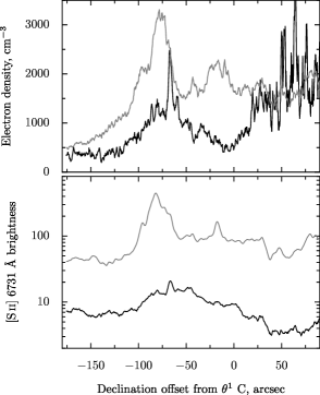
Figure 9.— North-South profiles of electron density (upper panel) and [$\mathrm{S\,\scriptstyle II}$] surface brightness (lower panel) from a slit situated $40.5\arcsec{}$ E of $\theta^{1}$Ori C. The black lines show emission at velocities around that of the blueshifted line component ($-7$ to $+7$ $\mathrm{km\ s}^{-1}$) while the gray lines show emission from the principal line component ($+7$ to $+50~{}\mathrm{km\ s}^{-1}{}$).

A notable property of the [$\mathrm{S\,\scriptstyle II}$] profiles in the southeastern region of the nebula (Fig. 1cd) is that they are double-peaked, showing a well-defined secondary emission component centered on $V_{\odot}\simeq-2~{}\mathrm{km\ s}^{-1}$, which is 20–25 $\mathrm{km\ s}^{-1}$ to the blue of the main component. This component is not detected in [$\mathrm{O\,\scriptstyle I}$] or [$\mathrm{S\,\scriptstyle III}$], although to the north of the Bright Bar it merges with emission from the Big Arc, which is also visible in [$\mathrm{S\,\scriptstyle III}$]. The spatial distribution of this component, which we will call the Diffuse Blue Layer, can be appreciated as the extended green emission in the lower left corner of the [$\mathrm{S\,\scriptstyle II}$] image of Figure 3. The electron density of this layer is very low, as can be seen from Figure 5.

In the lower panel of Figure 9 we show brightness profiles for red and blue velocity ranges of the [$\mathrm{S\,\scriptstyle II}$] 6731 Å line for a representative slit in the East of the nebula. The blue channel covers velocities $-7$ to $+7$ $\mathrm{km\ s}^{-1}$ while the red channel covers velocities $+7$ to $+50~{}\mathrm{km\ s}^{-1}{}$. The Diffuse Blue Layer is the dominant contribution to the blue channel brightness south of an offset of $-100$. The upper panel shows that the density of the Layer is roughly constant at $n_{\mathrm{e}}\simeq 400~{}\mathrm{cm}^{-3}$. The Bright Bar crosses the slit for positions between $-75$ and $-100$ and the brightness of the systemic nebular component becomes so large that its wing also dominates the brightness in the blue channel. Slightly further to the north, a peak in blue channel brightness occurs where the Big Arc crosses the slit. Therefore, the density rise in the blue channel that is seen between positions of $-100$ and $-25$ is not due to the Diffuse Blue Layer itself. To the north of the Big Arc, between offsets of $-25$ and $0$, the Diffuse Blue Layer again dominates the blue channel and the density returns to $\simeq 500~{}\mathrm{cm}^{-3}$. Further to the north, the intensity of the Diffuse Blue Layer declines and the wing of the systemic component returns to dominate the blue channel.

To the west of the nebula, the Diffuse Blue Layer is much less prominent and is only detectable to the south of the Bright Bar. A dark band appears to cross the Diffuse Blue Layer in the $-12~{}\mathrm{km\ s}^{-1}{}$ channel, roughly parallel to the ionization front of the Bright Bar but about 15″ farther away from the Trapezium.

One of our [$\mathrm{S\,\scriptstyle II}$] slits reaches 40″ farther north than the area covered by our maps and shows that a similar feature to the Diffuse Blue Layer reappears around ($+49$, $+156$). The density is $n_{\mathrm{e}}\simeq 500~{}\mathrm{cm}^{-3}$ but the velocity is slightly redder at $V_{\odot}\simeq+9~{}\mathrm{km\ s}^{-1}{}$, although it is still well separated from the systemic component, which lies at $+24~{}\mathrm{km\ s}^{-1}{}$ with $n_{\mathrm{e}}\simeq 1300~{}\mathrm{cm}^{-3}$.

We do not detect this component in [$\mathrm{O\,\scriptstyle I}$] or [$\mathrm{S\,\scriptstyle III}$] but it can also be seen in [$\mathrm{N\,\scriptstyle II}$] (Henney & O’Dell, 1999) and in [$\mathrm{O\,\scriptstyle II}$] 3727, 3729 Å (Jones, 1992). The Henney & O’Dell observations show it to extend at least another 20″ east of the region covered by our maps. It seems likely that this component is the same as that identified many years ago as a region of line splitting in [$\mathrm{N\,\scriptstyle II}$] (Deharveng, 1973). The region around and to the south of the Bright Bar coincides with Deharveng’s Region A, while the similar feature found to the North is part of her Region B. A third region of splitting (Region C) in the far west of the nebula lies outside the area of our observations.

The lack of [$\mathrm{O\,\scriptstyle I}$] emission suggests that this emission does not come from an ionization front, but rather from an extended region of fully ionized gas. The lack of [$\mathrm{S\,\scriptstyle III}$] emission implies that helium is neutral and that the ionizing spectrum is rather soft. It is therefore possible that the Blue Layer is due to a separate region along the line of sight that is ionized by $\theta^{2}$Ori A instead of by $\theta^{1}$Ori C. This is also consistent with the spatial distribution of the layer in the south east (Deharveng’s Region A). However, the larger scale distribution of the [$\mathrm{N\,\scriptstyle II}$] line splitting mapped by Deharveng (1973) argues instead that the Blue Layer is instead related to the large-scale champagne flow from the nebula.

4. Conclusions

We have mapped the Orion Nebula in a variety of optical emission lines in order to produce images of the region that are resolved in both velocity and in ionization. We have also produced the first velocity-resolved electron density maps of the nebula. The spatio-kinematic information revealed by our maps sheds new light on previously known nebular features and also uncovers several new components of the nebula. In this paper, we concentrate on low ionization emission within $\pm 40~{}\mathrm{km\ s}^{-1}$ of the systemic velocity and our main conclusions are:

1. We find a region to the east and southeast of the Trapezium, which we call the Red Bay, where the usual correlation between velocity and ionization potential is very weak or absent and where the emission layer is much thicker along the line of sight than in the west of the nebula. This is gas that is not sharing in the general champagne flow of the nebula, presumably beacause of the local concave geometry of the ionization front in the region.

2. We find an extensive layer of low-density, low-ionization, blueshifted emission in the southeast of the nebula, which may be ionized by the softer spectrum of the nearby O9.5 star $\theta^{2}$Ori A, or may represent the near side of the champagne flow from the nebula.

3. We detect a new redshifted jet, HH 873, to the southwest of the Trapezium, and a dense low-ionization shell that may represent an outer bowshock in the HH 203/204 flow.

Appendix A Translation between the coordinates used in the current paper and those of O’Dell & Wen (1994)

In the literature it is common for objects in the Orion nebula to be designated by a six-digit coordinate-based code of the form XXX–YZZ, which was first introduced by O’Dell & Wen (1994) and which is based on a truncated form of their J2000 positions, rounded to $0.1$ seconds in RA and $1\arcsec$ in declination (e.g., DOH04). For example, in this system, $\theta^{1}$Ori C would have the designation 165–323. In the current paper, we do not use this system, preferring instead to simply give arcsecond offsets ($x$, $y$) with respect to $\theta^{1}$Ori C.

In order to ease the comparison of our results with those of other papers, we here provide equations to transform between the two coordinate systems. The transformation between our ($x$, $y$) offsets and O’Dell & Wen’s system is

$$\mathrm{XXX} = \lfloor 164.6-0.6696\,x\rfloor$$

$$\mathrm{Y} = \lfloor(203.2-y)/60\rfloor$$

$$\mathrm{ZZ} = \lfloor 203.2-y\rfloor-60\,\mathrm{Y},$$

in which the notation $\lfloor\cdots\rfloor$ denotes the integer part, padded with leading zeros to the requisite number of digits. The inverse transformation is

$$x = 245.8-1.493\,\mathrm{XXX}$$

$$y = 203.2-(60\,\mathrm{Y}+\mathrm{ZZ}).$$

Note that these equations are only valid for right ascensions between 05^h 35^m and 05^h 36^m and declinations south of $-05\arcdeg{}\ 20\arcmin{}$, which corresponds to $-650<x<246$ and $y<203$. All our observations fall well within these limits.

References

- Baldwin et al. (1991) Baldwin, J. A., Ferland, G. J., Martin, P. G., Corbin, M. R., Cota, S. A., Peterson, B. M., & Slettebak, A. 1991, ApJ, 374, 580
- Baldwin et al. (2000) Baldwin, J. A., Verner, E. M., Verner, D. A., Ferland, G. J., Martin, P. G., Korista, K. T., & Rubin, R. H. 2000, ApJS, 129, 229
- Bally et al. (2000) Bally, J., O’Dell, C. R., & McCaughrean, M. J. 2000, AJ, 119, 2919
- Campbell & Moore (1918) Campbell, W. W., & Moore, J. H. 1918, Pub. Lick Obs., 13
- Castañeda & O’Dell (1987) Castañeda, H. O. & O’Dell, C. R. 1987, ApJ, 315, L55
- Cerqueira & de Gouveia Dal Pino (2004) Cerqueira, A. H. & de Gouveia Dal Pino, E. M. 2004, A&A, 426, L25
- Deharveng (1973) Deharveng, L. 1973, A&A, 29, 341
- de La Fuente et al. (2003) de La Fuente, E., Rosado, M., Arias, L., & Ambrocio-Cruz, P. 2003, Revista Mexicana de Astronomia y Astrofisica, 39, 127
- Doi et al. (2002) Doi, T., O’Dell, C. R., & Hartigan, P. 2002, AJ, 124, 445
- Doi et al. (2004) —. 2004, AJ, 127, 3456
- Elliott & Meaburn (1974) Elliott, K. H., & Meaburn, J. 1974, Ap&SS, 28, 351
- Esteban et al. (1998) Esteban, C., Peimbert, M., Torres-Peimbert, S., & Escalante, V. 1998, MNRAS, 295, 401
- Goudis (1982) Goudis, C. 1982, “The Orion complex: A case study of interstellar matter” (Dordrecht, Netherlands: D. Reidel Publishing Co.) Astrophysics and Space Science Library, Volume 90
- Goudis et al. (1984) Goudis, C., Hippelein, H., Meaburn, J., & Songsathaporn, R. 1984, A&A, 137, 245
- Graham et al. (2002) Graham, M. F., Meaburn, J., Garrington, S. T., O’Brien, T. J., Henney, W. J., & O’Dell, C. R. 2002, ApJ, 570, 222
- Hanel (1987) Hanel, A. 1987, A&A, 176, 347
- Henney (1998) Henney, W. J. 1998, ApJ, 503, 760
- Henney et al. (2005) Henney, W. J., Arthur, S. J., & García-Díaz, M. T. 2005, ApJ, 627, 813
- Henney & García-Díaz (2006) Henney, W. J. & García-Díaz, M. T. 2006, AJ, in preparation (Paper II)
- Henney & O’Dell (1999) Henney, W. J. & O’Dell, C. R. 1999, AJ, 118, 2350
- Henney et al. (2002) Henney, W. J., O’Dell, C. R., Meaburn, J., Garrington, S. T., & Lopez, J. A. 2002, ApJ, 566, 315
- Henney et al. (2006) Henney, W. J., O’Dell, C. R., Zapata, L. A., García-Díaz, M. T., Rodríguez, L. F., & Robberto, M. 2006, AJ, submitted
- Hester et al. (1991) Hester, J. J., et al. 1991, ApJ, 369, L75
- Hester & Desch (2005) Hester, J. J. & Desch, S. J. 2005, in ASP Conf. Ser. 341: Chondrites and the Protoplanetary Disk, 107
- Hillenbrand (1997) Hillenbrand, L. A. 1997, AJ, 113, 1733
- Hillenbrand & Carpenter (2000) Hillenbrand, L. A. & Carpenter, J. M. 2000, ApJ, 540, 236
- Hillenbrand & Hartmann (1998) Hillenbrand, L. A. & Hartmann, L. W. 1998, ApJ, 492, 540
- Høg et al. (2000) Høg, E., Fabricius, C., Makarov, V. V., Urban, S., Corbin, T., Wycoff, G., Bastian, U., Schwekendiek, P., & Wicenec, A. 2000, A&A, 355, L27
- Israel (1978) Israel, F. P. 1978, A&A, 70, 769
- Johnstone & Bally (1999) Johnstone, D. & Bally, J. 1999, ApJ, 510, L49
- Jones & Walker (1988) Jones, B. F. & Walker, M. F. 1988, AJ, 95, 1755
- Jones (1992) Jones, M. R. 1992, PhD thesis, Rice University
- Joye & Mandel (2003) Joye, W. A. & Mandel, E. 2003, in ASP Conf. Ser. 295: Astronomical Data Analysis Software and Systems XII, 489–+
- Leroy & Le Borgne (1987) Leroy, J. L. & Le Borgne, J. F. 1987, A&A, 186, 322
- Lim (2001) Lim, A. J. 2001, MNRAS, 327, 507
- Massey & Meaburn (1993) Massey, R. M. & Meaburn, J. 1993, MNRAS, 262, L48
- Massey & Meaburn (1995) —. 1995, MNRAS, 273, 615
- Meaburn et al. (2003) Meaburn, J., López, J. A., Gutiérrez, L., Quiróz, F., Murillo, J. M., Valdéz, J., & Pedrayez, M. 2003, Revista Mexicana de Astronomia y Astrofisica, 39, 185
- Meaburn et al. (1993) Meaburn, J., Massey, R. M., Raga, A. C., & Clayton, C. A. 1993, MNRAS, 260, 625
- Mellema et al. (2006) Mellema, G., Arthur, S. J., Henney, W. J., Iliev, I. T., & Shapiro, P. R. 2006, ApJ, 647, 397
- O’Dell (2001) O’Dell, C. R. 2001, ARA&A, 39, 99
- O’Dell & Bally (1999) O’Dell, C. R. & Bally, J. 1999, in ASP Conf. Ser. 188: Optical and Infrared Spectroscopy of Circumstellar Matter, 25–+
- O’Dell et al. (2001) O’Dell, C. R., Ferland, G. J., & Henney, W. J. 2001, ApJ, 556, 203
- O’Dell et al. (1997a) O’Dell, C. R., Hartigan, P., Bally, J., & Morse, J. A. 1997a, AJ, 114, 2016
- O’Dell et al. (1997b) O’Dell, C. R., Hartigan, P., Lane, W. M., Wong, S. K., Burton, M. G., Raymond, J., & Axon, D. J. 1997b, AJ, 114, 730
- O’Dell et al. (1993) O’Dell, C. R., Valk, J. H., Wen, Z., & Meyer, D. M. 1993, ApJ, 403, 678
- O’Dell et al. (1992) O’Dell, C. R., Walter, D. K., & Dufour, R. J. 1992, ApJ, 399, L67
- O’Dell & Wen (1992) O’Dell, C. R. & Wen, Z. 1992, ApJ, 387, 229
- O’Dell & Wen (1994) —. 1994, ApJ, 436, 194
- O’Dell & Yusef-Zadeh (2000) O’Dell, C. R. & Yusef-Zadeh, F. 2000, AJ, 120, 382
- Pogge et al. (1992) Pogge, R. W., Owen, J. M., & Atwood, B. 1992, ApJ, 399, 147
- Raju et al. (1993) Raju, K. P., Prasad, C. D., Desai, J. N., & Mishra, L. 1993, Ap&SS, 204, 205
- Rosado et al. (2001) Rosado, M., de la Fuente, E., Arias, L., Raga, A., & Le Coarer, E. 2001, AJ, 122, 1928
- Smith et al. (2004) Smith, N., Bally, J., Shuping, R. Y., Morris, M., & Hayward, T. L. 2004, ApJ, 610, L117
- Tenorio-Tagle (1979) Tenorio-Tagle, G. 1979, A&A, 71, 59
- Wen & O’Dell (1993) Wen, Z. & O’Dell, C. R. 1993, ApJ, 409, 262
- Werner et al. (1976) Werner, M. W., Gatley, I., Becklin, E. E., Harper, D. A., Loewenstein, R. F., Telesco, C. M., & Thronson, H. A. 1976, ApJ, 204, 420
- Wilson et al. (1959) Wilson, O. C., Münch, G., Flather, E., & Coffeen, M. F. 1959, ApJS, 4, 199
- Wilson et al. (1997) Wilson, T. L., Filges, L., Codella, C., Reich, W., & Reich, P. 1997, A&A, 327, 1177
- Yorke (1986) Yorke, H. W. 1986, ARA&A, 24, 49
- Zuckerman (1973) Zuckerman, B. 1973, ApJ, 183, 863