Variational Integrators for the Gravitational $N$-Body Problem

Abstract

This paper describes a fourth-order integration algorithm for the gravitational $N$-body problem based on discrete Lagrangian mechanics. When used with shared timesteps, the algorithm is momentum conserving and symplectic. We generalize the algorithm to handle individual time steps; this introduces fifth-order errors in angular momentum conservation and symplecticity. We show that using adaptive block power of two timesteps does not increase the error in symplecticity. In contrast to other high-order, symplectic, individual timestep, momentum-preserving algorithms, the algorithm takes only forward timesteps. We compare a code integrating an $N$-body system using the algorithm with a direct-summation force calculation to standard stellar cluster simulation codes. We find that our algorithm has about 1.5 orders of magnitude better symplecticity and momentum conservation errors than standard algorithms for equivalent numbers of force evaluations and equivalent energy conservation errors.

1 Introduction

The gravitational $N$-body problem is the numerical integration of trajectories for $N$ particles with pairwise inverse square-law forces. Ideally, a numerical method should respect all of the symmetries of the exact problem. Conservation of linear and angular momentum and energy — in toto or in pairwise interactions — are often used as quality indicators for numerical algorithms. However, there is another conservation law following from Hamiltonian dynamics: conservation of the symplectic form on phase space.

Symplectic integration methods conserve exactly the symplectic form. This leads to other desirable properties of the flow of the integrator; for example, symplecticity implies incompressible, or dissipation less, flow. Symplectic methods are well known in numerical integration of the solar system following the pioneering work of Wisdom & Holman (1991). However, the advantages of symplectic methods apply to systems with many more bodies. Indeed, cosmological simulations with millions or even billions of particles often use the leapfrog method because of its symplectic behavior (Springel, 2005b; Shirokov & Bertschinger, 2005).

The leapfrog algorithm is second-order accurate. Higher-order accurate compositional algorithms are possible but conventionally require sub-steps integrated backwards in time (Yoshida, 1993; Chambers, 2003) and such techniques typically require many more force evaluations than standard integrators. Symplectic implicit Runge-Kutta-Nyström integrators are well-known, and involve relatively few force evaluations (Suris, 1989; Marsden & West, 2001; Stuchi, 2002).

Gravitating systems typically have a large dynamic range of density and hence dynamical time, making it computationally inefficient to use a constant timestep, as required by most symplectic algorithms. Either adaptive timesteps (which change with time as a system evolves), individual timesteps (which differ for each particle), or both are required to make a computation feasible. This is especially true when unsoftened inverse-square law forces are used, e.g., in numerical simulation of globular clusters (Heggie & Hut, 2003). It is well-known how to use compositional symplectic algorithms with individual timesteps (Springel, 2005b), but the larger number of force evaluations in the high-order compositional algorithms and the necessity of backward sub-steps rule these out for use in simulations of large-$N$ gravitating systems (Springel, 2005a). No individual timestepping symplectic Runge-Kutta-Nyström algorithm has appeared previously in the literature.

Below we describe a fourth-order symplectic Runge-Kutta-Nyström algorithm from a variational point of view. The algorithm requires the solution of a nonlinear algebraic equation for one forwards sub-step. If the nonlinear equation is solved approximately by iteration then the algorithm is approximately symplectic with an error in phase space conservation that can be made arbitrarily small. We describe how to use data from the last step of the integrator to generate an approximate solution sufficient to obtain fifth-order symplecticity and momentum-conservation using only two force evaluations per step. We generalize this algorithm to use individual (and adaptive) timesteps; the formulation in terms of a discretized action principle is essential to the generalization. This is the first individual timestepping symplectic Runge-Kutta-Nyström algorithm to appear in the astrophysical literature.

It is widely believed that adaptive timesteps are incompatible with symplecticity but we show otherwise in Section 4. This assumed breakdown of symplecticity, coupled with the large number of force evaluations for standard higher-order compositional symplectic methods and the lack of individual timestepping symplectic Runge-Kutta-Nyström algorithms, has led researchers to seek alternative ways to reduce dissipation, e.g. using time-reversible integration (Makino et al., 1996; Preto & Tremaine, 1999). These techniques treat the symptoms of non-symplecticity (linear growth in various errors) without treating the cause (non-conservation of the symplectic form). Our algorithm addresses the cause, and we see corresponding improvements in symplecticity and momentum conservation for equivalent energy error to relative standard algorithms.

In this paper we present a fourth-order integrator requiring only two force evaluations per timestep, which is fifth-order in symplecticity. Each additional force evaluation improves the symplecticity by two powers of the timestep. We generalize the integrator to individual timesteps and analyze the breakdown of symplecticity when adaptive and individual timesteps are used. We show that symplecticity is effectively restored when block power of two timesteps are used.

The algorithm is based on a discrete approximation to the action of a system, described in Section 2. The algorithm contains a non-linear equation whose solution must be approximated; we compare two approximation methods in Section 3. Adaptive, individual, and combined block timesteps are discussed in Sections 4, 5, and 6 respectively. Numerical tests are presented in Section 7. Conclusions are given in Section 8.

2 Variational Integrators

Variational integrators are based on applying Hamilton’s principle of stationary action to discrete approximations to the action for a physical system. Lew et al. (2004) is an excellent introduction to variational integrators in an engineering context; Marsden & West (2001) provides a much more mathematical discussion, including proofs of the essential properties of variational integrators and many examples of particular integration rules. This section is a brief introduction to variational integrators. Here and throughout we suppress vector indices on variables (juxtaposition of variables thus denotes multiplication in the one-dimensional case and the usual dot-product in the multidimensional case). We denote the derivative of the function $f$ by $Df$; we denote the partial derivative on the $i$th argument of the function $g$ by $\partial_{i}g$ (argument labels begin at 0).

The fundamental theorem of variational integration (Marsden & West, 2001, Theorem 2.3.1) states that if $H$ is an approximation to the action of a mechanical system,

$$H(h,q_{1},q^{\prime},q^{\prime\prime},\ldots,q^{(n)},q_{2})=S[q](t_{1},t_{1}+h)+\mathcal{O}(h^{r+1})=\int_{t_{1}}^{t_{1}+h}dt\,L(t,q(t),Dq(t))+\mathcal{O}(h^{r+1}),$$ (1)

where $q_{1}=q(t_{1})$, $q_{2}=q(t_{2})$, the $q^{(i)}$ are intermediate positions in the time interval $[t_{1},t_{1}+h]$, $S$ is the action functional and $L$ is the Lagrangian for the system, then the equations

$$\partial_{1}H(h,q_{1},q^{\prime},q^{\prime\prime},\ldots,q^{(n)},q_{2}) = -p_{1}$$ (2a)

$$\partial_{i}H(h,q_{1},q^{\prime},q^{\prime\prime},\ldots,q^{(n)},q_{2}) = 0,\qquad i=2,3,\ldots,n+1$$ (2b)

$$\partial_{n+2}H(h,q_{1},q^{\prime},q^{\prime\prime},\ldots,q^{(n)},q_{2}) = p_{2}$$ (2c)

define a map $(q_{1},p_{1})\mapsto(q_{2},p_{2})$ which is an order $r$ integrator for the mechanical system. The function $H$ is called the discrete Lagrangian. Equations (2b) extremize the discrete action approximation with respect to the discrete path $\{q^{(i)}\}$, while equations (2a) and (2c) exploit that the action is a $F_{1}$-type generating function for the time-evolution canonical transformation (Sussman et al., 2001, pp. 415–416).

The map defined by equations (2) has many useful properties analogous to the properties of the exact evolution of the system defined by $L$. First, it is momentum-preserving: imagine an infinitesimal variation in the coordinates $q_{1}$, $q_{2}$ and $q^{(i)}$ which leaves $H$ invariant when $q_{1}$, the $q^{(i)}$ and $q_{2}$ satisfy equations (2). We have

$$\delta H = \partial_{1}H(h,q_{1},q^{\prime},q^{\prime\prime},\ldots,q^{(n)},q_{2})\delta q_{1}+\sum_{i=2}^{n+1}\partial_{i}H(h,q_{1},q^{\prime},q^{\prime\prime},\ldots,q^{(n)},q_{2})\delta q^{(i)}$$ (3)

$$\mbox{}+\partial_{n+2}H(h,q_{1},q^{\prime},q^{\prime\prime},\ldots,q^{(n)},q_{2})\delta q_{2}$$

$$= p_{2}\delta q_{2}-p_{1}\delta q_{1}$$

$$= 0.$$

In this situation the quantity $p\delta q$ is conserved by the integrator: this is the discrete version of Nöther’s theorem. Assuming that $H$ inherits the symmetries of $L$, the integrator will exactly preserve the associated discrete momenta.

Second, the map is symplectic. Consider the discrete approximation to the action over an interval evaluated on the integrator path:

$$\mathcal{S}\left(q_{1},q_{2},\ldots,q_{M}\right)\equiv\sum_{i=1}^{M-1}H\left(h,q_{i},q^{\prime}_{i},\ldots,q^{(n)}_{i},q_{i+1}\right),$$ (4)

where the $q_{i}$ satisfy the integrator equations (2). Taking one exterior derivative of $\mathcal{S}$ gives

$$d\mathcal{S}\left(q_{1},q_{2},\ldots,q_{M}\right) = \partial_{1}H\left(h,q_{1},q^{\prime}_{1},\ldots,q^{(n)}_{1},q_{2}\right)dq_{1}$$ (5)

$$\mbox{}+\partial_{n+2}H\left(h,q_{M-1},q^{\prime}_{M-1},\ldots,q^{(n)}_{M-1},q_{M}\right)dq_{M};$$

the terms involving $dq_{2},\ldots,dq_{M-1}$ are identically zero because the trajectory satisfies equations (2a), (2b) and (2c). Two exterior derivatives of $\mathcal{S}$ give zero, yielding

$$d^{2}\mathcal{S}\left(q_{1},q_{2},\ldots,q_{M}\right) = \partial_{1}\partial_{n+2}H\left(h,q_{1},q^{\prime}_{1},\ldots,q^{(n)}_{1},q_{2}\right)dq_{1}\wedge dq_{2}$$ (6)

$$\mbox{}+\partial_{1}\partial_{n+2}H\left(h,q_{M-1},q^{\prime}_{M-1},\ldots,q^{(n)}_{M-1},q_{M}\right)dq_{M}\wedge dq_{M-1}$$

$$= 0.$$

Instead of considering evolution on phase space $(q,p)$, consider the corresponding evolution on the discrete state space $\left(q_{1},q_{2}\right)$. Evolution maps the initial state-space for $H$, $\left(q_{1},q_{2}\right)\in\mathbb{R}^{m}\times\mathbb{R}^{m}$, to an isomorphic space, $\left(q_{M-1},q_{M}\right)\in\mathbb{R}^{m}\times\mathbb{R}^{m}$, where $m$ is the dimensionality of configuration space. Equation (6) can be written

$$\partial_{1}\partial_{n+2}H\left(h,q_{1},q^{\prime}_{1},\ldots,q^{(n)}_{1},q_{2}\right)dq_{1}\wedge dq_{2}=F^{*}\left[\partial_{1}\partial_{n+2}H\left(h,q_{1},q^{\prime}_{1},\ldots,q^{(n)}_{1},q_{2}\right)dq_{1}\wedge dq_{2}\right]$$ (7)

using the pushforward map under evolution, $F^{*}$. All forms in equation (7) live on the cotangent bundle of the state space $\mathbb{R}^{m}\times\mathbb{R}^{m}$. We see that the integrator conserves the discrete symplectic form on the state space of $H$,

$$\partial_{1}\partial_{n+2}H\left(h,q_{1},q^{\prime}_{1},\ldots,q^{(n)}_{1},q_{2}\right)dq_{1}\wedge dq_{2}.$$ (8)

This is the direct analog of the symplecticity of continuous time-evolution in a Hamiltonian system.

Using equation (2a), we see that

$$-dp_{1}=\partial_{1}\partial_{1}H(h,q_{1},q^{\prime},q^{\prime\prime},\ldots,q^{(n)},q_{2})dq_{1}+\partial_{n+2}\partial_{1}H(h,q_{1},q^{\prime},q^{\prime\prime},\ldots,q^{(n)},q_{2})dq_{2},$$ (9)

and therefore conservation of the discrete symplectic form in equation (8) implies conservation of the Poincaré integral invariant on phase space:

$$\partial_{1}\partial_{n+2}H\left(h,q_{1},q^{\prime}_{1},\ldots,q^{(n)}_{1},q_{2}\right)dq_{1}\wedge dq_{2}=dp_{1}\wedge dq_{1}.$$ (10)

Finally, while it is impossible for a constant-time-stepping integrator to be momentum-conserving, symplectic and to exactly conserve energy (Ge & Marsden, 1988), variational integrators generally have bounded energy error. Lew et al. (2004) explain that the discretized trajectory is sampling the continuous trajectory of a Lagrangian system, $\tilde{L}$, which is near $L$. $\tilde{L}$ satisfies

$$\int_{t_{1}}^{t_{1}+h}dt\,\tilde{L}(t,q(t),Dq(t))=H\left(h,q_{1},q^{\prime},q^{\prime\prime},\ldots,q^{(n)},q_{2}\right),$$ (11)

where the integral is evaluated on the trajectory which satisfies the Euler-Lagrange equations for $\tilde{L}$ with $q\left(t_{1}\right)=q_{1}$ and $q\left(t_{1}+h\right)=q_{2}$ and the positions which are arguments for $H$ satisfy equations (2). Equation (11) implies that $H$ is the exact generating function for time evolution under $\tilde{L}$. In general it is only possible to compute a truncation of $\tilde{L}$ to any desired order in $h$, but it is possible to prove that $\tilde{L}$ is close to $L$ in the space of possible Lagrangians. Since the trajectory remains on the energy level set of $\tilde{L}$ in phase space, near the energy level-set for $L$, the energy error remains bounded.

2.1 Galerkin Gauss-Lobatto Variational Integrators

To define a variational integrator, we need an $H$-type function which approximates the action for a system over an interval. There are many ways to find such a function; see Marsden & West (2001) for an extensive discussion of the various types of integrator. In this paper, we will focus on the so-called Galerkin Gauss-Lobatto (GGL) integrators. These integrators assume a polynomial trajectory in time and approximate the action integral using a Gauss-Lobatto quadrature rule. Gauss-Lobatto quadrature is appropriate because it gives the highest-order integration rule for a given number of points subject to the constraint that the Lagrangian is evaluated once at the beginning and once at the end of the interval. Evaluating at the beginning and end of the interval is important because it preserves the symmetries of the continuous Lagrangian.

Marsden & West (2001) show that all GGL integrators can be written as symplectic partitioned Runge-Kutta integrators and derive formulas which relate the SPRK coefficients to the discrete Lagrangian. Because variational integrators are symplectic, GGL integrators automatically satisfy the constraints on symplectic Runge-Kutta coefficients (see, for example, Suris (1989); Marsden & West (2001); Stuchi (2002)). The particular integration algorithms we consider here belong to a sub-class of partitioned Runge-Kutta methods often called Runge-Kutta-Nyström methods.

We define

$$H(h,q_{1},q^{\prime},\ldots,q^{(n)},q_{2})\equiv$$ (12)

$$w_{1}L(t_{1},\phi(t_{1},q_{1},q^{\prime},\ldots,q^{(n)},q_{2},t_{1},h),\partial_{0}\phi(t_{1},q_{1},q^{\prime},\ldots,q^{(n)},q_{2},t_{1},h))$$

$$\mbox{}+\sum_{i=1}^{n}w^{(i)}L(t^{(i)},\phi(t^{(i)},q_{1},q^{\prime},\ldots,q^{(n)},q_{2},t_{1},h),\partial_{0}\phi(t^{(i)},q_{1},q^{\prime},\ldots,q^{(n)},q_{2},t_{1},h))$$

$$\mbox{}+w_{2}L(t_{1}+h,\phi(t_{1}+h,q_{1},q^{\prime},\ldots,q^{(n)},q_{2},t_{1},h),\partial_{0}\phi(t_{1}+h,q_{1},q^{\prime},\ldots,q^{(n)},q_{2},t_{1},h)),$$

where $\phi(t,q_{1},q^{\prime},\ldots,q^{(n)},q_{2},t_{1},h)$ is the interpolating polynomial for $q(t)$ passing through the points $\{q_{1},q^{\prime},\ldots,q^{(n)},q_{2}\}$ at times $\{t_{1},t^{\prime},\ldots,t^{(n)},t_{1}+h\}$. The times $\{t_{1},t^{\prime},\ldots,t^{(n)},t_{1}+h\}$ and weights $\{w_{1},w^{\prime},\ldots,w^{(n)},w_{2}\}$ define the $n+2$ point Gauss-Lobatto quadrature rule. This rule is exact for quadrature of polynomials up to and including order $2n+2$. The integrator so defined will be of order $2n+2$. See, for example, Abramowitz & Stegun (1972, Table 25.6) for appropriate times and weights. This is easier than it looks; examples follow.

2.1.1 Two-Point Integrator

The two-point Gauss-Lobatto integration rule has times $\{t_{1},t_{1}+h\}$ and weights $\{h/2,h/2\}$; a two-point interpolating polynomial is a line. Therefore, we have

$$H(h,q_{1},q_{2})=\frac{h}{2}\left[L\left(t_{1},q_{1},\frac{q_{2}-q_{1}}{h}\right)+L\left(t_{1}+h,q_{2},\frac{q_{2}-q_{1}}{h}\right)\right].$$ (13)

For a Lagrangian $L(t,q,v)=\frac{1}{2}mv^{2}-V(q)$, equations (2a) and (2c) result in the explicit integration rule

$$q_{2} = q_{1}+h\frac{p_{1}}{m}-\frac{h^{2}}{2m}DV(q_{1})$$ (14a)

$$p_{2} = p_{1}-\frac{h}{2}\left[DV\left(q_{1}\right)+DV\left(q_{2}\right)\right].$$ (14b)

This rule is kick-drift-kick leapfrog; it can be derived from the Hamiltonian viewpoint by iterating the evolutions of the splitting of the Hamiltonian for this system into $H_{1}(q,p)=V(q)$ and $H_{2}(q,p)=p^{2}/(2m)$ (for a thorough exploration of this idea see, for example, Wisdom & Holman (1991) and Yoshida (1993)). This rule is second order, as expected from the order of the quadrature rule.

2.1.2 Three-Point Integrator

The three-point Gauss-Lobatto quadrature rule has times $\{t_{1},t_{1}+h/2,t_{1}+h\}$ and weights $\{h/6,2h/3,h/6\}$. The three-point interpolation polynomial is quadratic in time. Applying equation (12), we find

$$H(h,q_{1},q^{\prime},q_{2}) = h\left[\frac{1}{6}L\left(t_{1},q_{1},\frac{4q^{\prime}-3q_{1}-q_{2}}{h}\right)\right.$$ (15)

$$\left.\mbox{}+\frac{2}{3}L\left(t_{1}+\frac{h}{2},q^{\prime},\frac{q_{2}-q_{1}}{h}\right)+\frac{1}{6}L\left(t_{1}+h,q_{2},\frac{q_{1}+3q_{2}-4q^{\prime}}{h}\right)\right].$$

If $L(t,q,v)=\frac{1}{2}mv^{2}-V(q)$ then equations (2a), (2b) and (2c) reduce to

$$q^{\prime} = q_{1}+\frac{h}{2}\frac{p_{1}}{m}-\frac{1}{2}\left(\frac{h}{2}\right)^{2}\left[\frac{2DV\left(q_{1}\right)}{3m}+\frac{DV\left(q^{\prime}\right)}{3m}\right]$$ (16a)

$$q_{2} = q_{1}+h\frac{p_{1}}{m}-\frac{1}{2}h^{2}\left[\frac{DV\left(q_{1}\right)}{3m}+\frac{2DV\left(q^{\prime}\right)}{3m}\right]$$ (16b)

$$p_{2} = p_{1}-h\left[\frac{DV\left(q_{1}\right)}{6}+\frac{2DV\left(q^{\prime}\right)}{3}+\frac{DV\left(q_{2}\right)}{6}\right]$$ (16c)

To implement this integration scheme, we must solve the implicit equation (16a) for $q^{\prime}$. In spaces of high dimensionality (i.e. an $N$-body system with large $N$), the only efficient way to do this is through iteration: we treat equation (16a) as a prescription for updating the value of $q^{\prime}$, and iterate. We describe two iteration techniques in the following section.

The three-point GGL integrators take only forward steps in time. It is not possible to write these integrators as iterated evolution of a splitting of the Hamiltonian corresponding to $L$ (as in the two-point case): a general theorem states that it is impossible to have evolution by Hamiltonian splitting which is higher than second-order accurate and takes only forward steps (Sheng, 1989; Suzuki, 1991).

It is possible to formulate higher-order mapping integrators from the Hamiltonian perspective which take only forward steps using the force gradient (Wisdom et al., 1996; Scuro & Chin, 2005; Chin & Chen, 2005), but force gradients can be expensive to compute. Omelyan (2006) describes how to approximate computation of a force gradient with an extra force evaluation at a shifted position. The iteration technique in Section 3.1 reproduces algorithm 8 in Omelyan (2006) from the equations (16a), (16b), and (16c). However, we find that for equivalent numbers of force evaluations in the $N$-body problem, the alternate iteration technique in Section 3.2 typically outperforms the one in Section 3.1 by one to two orders of magnitude in energy error (see Figure 1), so the gradient-approximating algorithm from Omelyan (2006) is sub-optimal for our purposes.

Forward time steps are important for cosmological simulations which include gas dynamics because such simulations are unstable under time reversal. The requirement of symplecticity and forward timesteps has previously restricted cosmological simulations to second-order mapping integrators (Springel, 2005a).

It is straightforward to derive the integration equations for $n+2$-point GGL integrators with $n>1$. All such integrators have implicit equations for the intermediate positions, $q^{\prime},\ldots,q^{(n)}$, which must be solved via iteration exactly as in the $n=1$ case discussed above. In the presence of individual timesteps (Section 5), we must predict the intermediate positions—we cannot iterate the implicit equations to convergence. For integrators of order greater than four, such predicted positions do not solve the implicit equations accurately enough to make the symplecticity error scale better than the trajectory error; as we shall see, we can predict the solution to equation (16a) accurately enough to produce fifth-order symplecticity error in the fourth-order integrator. For this reason, the fourth-order integrator is uniquely positioned in the hierarchy of GGL integrators for adaptation to individual timesteps

3 Solving the Implicit Equation

This section discusses two ways to solve equation (16a) with iteration. They differ in their choice of initial guess for $q^{\prime}$. The choice in Section 3.1 produces an algorithm which is compositional, and is equivalent to algorithm 8 from Omelyan (2006). That algorithm is exactly phase-space-volume and momentum conserving, but only fourth-order symplectic, with three force evaluations per step. The choice in Section 3.2 produces an algorithm which is fifth-order symplectic (and the same in phase-space-volume error), exactly conserves linear momentum, and conserves angular momentum at fifth-order, with two force evaluations per step.

Omelyan (2006) reports excellent energy conservation for the algorithm in Section 3.1 when simulating the one-dimensional Kepler problem (where phase-space-volume conservation implies symplecticity), but we find that the algorithm in Section 3.2 has one to two orders of magnitude better energy conservation for equivalent numbers of force evaluations in the $N$-body problem for $N>2$ (see Figure 1). This is probably due to the superior symplecticity of the algorithm in Section 3.2 for multidimensional configuration spaces. We do not discuss the generalization of the algorithm in Section 3.1 to individual and adaptive timesteps, but instead focus on the algorithm in Section 3.2 for the remainder of the paper.

3.1 Compositional Algorithm

To reproduce algorithm 8 in Omelyan (2006), let the initial guess for $q^{\prime}$ be

$$q^{\prime}_{(0)}=q_{1}+\frac{h}{2}\frac{p_{1}}{m}-\frac{1}{2}\left(\frac{h}{2}\right)^{2}\frac{2DV\left(q_{1}\right)}{3m}.$$ (17)

Then iterate equation (16a) once, producing

$$q^{\prime}=q^{\prime}_{(0)}-\frac{h^{2}}{24m}DV\left(q^{\prime}_{(0)}\right).$$ (18)

$q_{2}$ and $p_{2}$ are then given by equations (16b) and (16c), with this choice for $q^{\prime}$. This choice of initial guess and single iteration allows the algorithm to be written compositionally as

$$p \leftarrow p-\frac{h}{6}DV(q)$$ (19a)

$$q \leftarrow q+\frac{h}{2}\frac{p}{m}$$ (19b)

$$p \leftarrow p-\frac{2h}{3}DV\left(q-\frac{h^{2}}{24m}DV(q)\right)$$ (19c)

$$q \leftarrow q+\frac{h}{2}\frac{p}{m}$$ (19d)

$$p \leftarrow p-\frac{h}{6}DV(q).$$ (19e)

This is exactly the sequence of operations in Omelyan (2006), algorithm 8; equation (19c) is the approximation derived in Omelyan (2006) to the force gradient required in the corresponding algorithm of Chin & Chen (2005). The algorithm needs four force evaluations for a single step, but only three in a long-running simulation because the first force evaluation of a step occurs at the same position as the last force evaluation of the previous step. The algorithm exactly conserves phase-space volume and momentum, but is only fourth-order symplectic (in $2n$-dimensional phase-spaces with $n>1$). As stated above, in practice we find that the energy error from this algorithm in $N$-body simulations is significantly worse than that from the following algorithm. We compare the energy error behavior of the algorithms in Figure 1.

3.2 Prediction Algorithm

As we shall see in Section 5, it is not, in general, possible to iterate equation (16a) in the presence of individual timesteps. Iterating equation (16a) for a particle corresponds to re-running the evolution of that particle over the first half of its timestep. This may require re-running many entire steps of particles with smaller timesteps than the given particle, which, in turn, may require re-running yet more steps of particles with even smaller timesteps. The explosion of work is exponential in the number of distinct timesteps assigned to particles in the simulation.

Given that we cannot iterate equation (16a), it makes sense to try to use all the information at hand to predict the solution $q^{\prime}$ as well as possible at the beginning of a particle’s timestep. The initial guess

$$q^{\prime}_{(0)}=q_{1}+\frac{h}{2}\frac{p_{1}}{m}+\frac{1}{2}\left(\frac{h}{2}\right)^{2}F(t)+\frac{1}{6}\left(\frac{h}{2}\right)^{3}DF(t)+\frac{1}{12}\left(\frac{h}{2}\right)^{4}D^{2}F(t),$$ (20)

where $t$ is the time at which the particle is at position $q_{1}$, and $F(t)$ is the force on the particle as a function of time, solves equation (16a) with an error term of order $h^{5}$. (Note that the final term in equation (20) is twice what would be expected in a power series for $q(t+h/2)$.) We can use the force evaluations from the previous step, at times $t-h$, $t-h/2$ and $t$, to approximate $F(t)$, $DF(t)$ and $D^{2}F(t)$ to sufficient accuracy to compute equation (20) with no new force evaluations.

The integration algorithm

$$q_{2} = q_{1}+h\frac{p_{1}}{m}-\frac{1}{2}h^{2}\left[\frac{DV\left(q_{1}\right)}{3m}+\frac{2DV\left(q^{\prime}_{(0)}\right)}{3m}\right]$$ (21)

$$p_{2} = p_{1}-h\left[\frac{DV\left(q_{1}\right)}{6}+\frac{2DV\left(q^{\prime}_{(0)}\right)}{3}+\frac{DV\left(q_{2}\right)}{6}\right],$$ (22)

which is equations (16) with $q^{\prime}$ replaced by the predicted $q^{\prime}_{(0)}$ from equation (20), is fifth-order accurate in symplecticity and angular momentum conservation, exactly conserves linear momentum, and requires only two potential evaluations per step in a long-running simulation. It outperforms the algorithm in Section 3.1 in energy error for equivalent force evaluations by one to two orders of magnitude, as evidenced in Figure 1. This is the algorithm we shall discuss for the remainder of the paper.

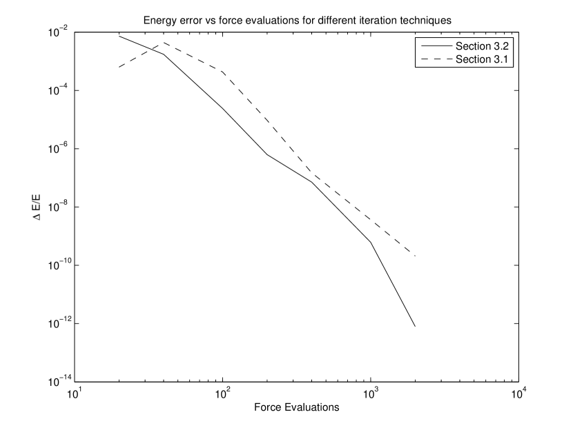
Figure 1: Energy error versus number of force evaluations for the algorithms described in Sections 3.1 and 3.2 in a simulation of a 100-body Plummer model initial condition with constant, shared timesteps over a total time interval $T=1.0$. As described in the text, the algorithm in Section 3.2 outperforms the compositional algorithm in Section 3.1 for equivalent numbers of potential evaluations, though both algorithms exhibit the same asymptotic scaling.

4 Adaptive Timesteps

In $N$-body simulations it is essential to be able to adapt the timestep taken by an integrator to the local conditions of the system. Formally, we can model such an adaptive step by treating the parameter $h$ in the discrete Lagrangian describing an integrator as a function of the positions through the step:

$$H\left(h,q_{1},q^{\prime}_{1},\ldots,q^{(n)}_{1},q_{2}\right)\to H\left(h\left(q_{1},q^{\prime}_{1},\ldots,q_{1}^{(n)},q_{2}\right),q_{1},q^{\prime}_{1},\ldots,q^{(n)}_{1},q_{2}\right).$$ (23)

Because the sequence of positions $q_{1},q^{\prime}_{1},\ldots,q_{1}^{(n)},q_{2}$ encodes all available information about the trajectory, essentially any technique for choosing a timestep can be recast in this fashion. We do not change the integrator equations

$$\partial_{1}H\left(h\left(q_{1},q^{\prime}_{1},\ldots,q^{(n)},q_{2}\right),q_{1},q^{\prime}_{1},\ldots,q^{(n)}_{1},q_{2}\right) = -p_{1}$$ (24)

$$\partial_{i}H\left(h\left(q_{1},q^{\prime}_{1},\ldots,q^{(n)},q_{2}\right),q_{1},q^{\prime}_{1},\ldots,q^{(n)}_{1},q_{2}\right) = 0,\qquad i=2,3,\ldots,n+1$$ (25)

$$\partial_{n+2}H\left(h\left(q_{1},q^{\prime}_{1},\ldots,q^{(n)},q_{2}\right),q_{1},q^{\prime}_{1},\ldots,q^{(n)}_{1},q_{2}\right) = p_{2}.$$ (26)

Assuming that the timestep function $h\left(q_{1},q^{\prime}_{1},\ldots,q_{1}^{(n)},q_{2}\right)$ is invariant under the same coordinate variations which leave $H$ invariant (this will be the case if both $H$ and $h$ inherit the same symmetries from the continuous Lagrangian), then the proof of momentum conservation in equation (3) still holds. All terms in $\delta H$ proportional to $\partial_{0}H\left(h\left(q_{1},q^{\prime}_{1},\ldots,q_{1}^{(n)},q_{2}\right),q_{1},q^{\prime}_{1},\ldots,q^{(n)}_{1},q_{2}\right)$ vanish because $\delta h$ also vanishes. Adaptive stepping poses no threat to momentum conservation, provided that the steps are chosen in a way which respects the symmetries in the continuous mechanical problem.

Unfortunately, adaptive stepping does pose a threat to symplecticity. With a timestep function $h\left(q_{1},q^{\prime}_{1},\ldots,q_{1}^{(n)},q_{2}\right)$, the expression for $d\mathcal{S}$ (see eq. (5)) gets additional terms:

$$\sum_{i=1}^{M-1}\partial_{0}H\left(h\left(q_{i},q^{\prime}_{i},\ldots,q_{i}^{(n)},q_{i+1}\right),q_{i},q^{\prime}_{i},\ldots,q_{i}^{(n)},q_{i+1}\right)$$ (27)

$$\mbox{}\times\left[\partial_{0}h\left(q_{i},q^{\prime}_{i},\ldots,q_{i}^{(n)},q_{i+1}\right)dq_{i}+\sum_{j=1}^{n}\partial_{j}h\left(q_{i},q^{\prime}_{i},\ldots,q_{i}^{(n)},q_{i+1}\right)dq^{(j)}_{i}\right.$$

$$\left.\mbox{}+\partial_{n+1}h\left(q_{i},q^{\prime}_{i},\ldots,q_{i}^{(n)},q_{i+1}\right)dq_{i+1}\right].$$

These extra terms prevent us from writing $d^{2}\mathcal{S}=0$ as the difference of two forms, one of which is the pushforward of the other, as we did in equation (7). With general adaptive timesteps, there is no two-form on the state space which is conserved over a fixed number of steps.

This can be understood intuitively in the following way. The conservation of the Poincaré integral invariant,

$$\mathcal{I}\equiv\sum_{i}dq^{i}\wedge dp_{i},$$ (28)

with the sum taken over coordinate dimensions, along any trajectory implies symplecticity (recall that eq. (10) shows that conservation of the two-form $\partial_{1}\partial_{n+2}H\left(h,q_{1},q^{\prime}_{1},\ldots,q_{1}^{(n)},q_{2}\right)dq_{1}\wedge dq_{2}$ on state space implies conservation of $\mathcal{I}$ on phase space). Note that $dq^{i}$ and $dp_{i}$ are exterior derivatives and that $\mathcal{I}$ is a two-form. The Poincaré integral invariant measures the sum of the areas of a tube of trajectories infinitesimally near a reference trajectory projected onto the sub-phase-spaces $\left(q^{i},p_{i}\right)$. But an integrator with an adaptive timestep does not advance all trajectories in the tube with the same $h$. Even if we had an adaptive timestep integrator which implemented the exact, continuous evolution of the system it still would not conserve $\mathcal{I}$ over a single step—stopping the evolution of the different trajectories in the tube at different times spoils the symplecticity of the continuous evolution. For an adaptive timestep integrator symplecticity after a fixed number of steps is the wrong condition to consider. Rather, we should ask whether the integrator conserves the symplectic form over a fixed total time of evolution. In general, any well-behaved integrator (including a variational integrator with general adaptive stepsizes) which has trajectory error of order $h^{r}$ conserves the symplectic form at least to order $h^{r}$ in this sense.

For variational integrators which choose timesteps using the popular block-power-of-two scheme we can do better: these integrators conserve the symplectic form almost everywhere in phase space. In the block-power-of-two scheme, a function $h_{\rm{max}}\left(q_{1},q^{\prime}_{1},\ldots,q_{1}^{(n)},q_{2}\right)$ limits the maximum timestep; the actual timestep taken is rounded down from $h_{\rm{max}}$ to the nearest number of the form $T/2^{n}$, with $n$ an integer, and $T$ some total evolution interval. If the function $h_{\rm{max}}$ is continuous, about every point in state space for which $h_{\rm{max}}\left(q_{1},q^{\prime}_{1},\ldots,q_{1}^{(n)},q_{2}\right)\neq T/2^{n}$ for some $n$ there is an open neighborhood of points which round down to the same timestep. Thus, the actual timestep function $h\left(q_{1},q^{\prime}_{1},\ldots,q_{1}^{(n)},q_{2}\right)$ is piecewise-constant on state space, and the derivatives in equation (27) vanish almost everywhere on state space for each step. A variational integrator with adaptive block-power-of-two timesteps is therefore symplectic almost everywhere on state space because it is a composition of symplectic steps. (“Almost everywhere” should be taken in the mathematical sense of “except on a set of measure zero.”) In Section 7 we present numerical evidence of this phenomenon. Incidentally, block-power-of-two timesteps have advantages for parallelization which have led other authors to adapt time-symmetric methods to block-power-of-two timesteps (Makino et al., 1996). Variational integrators fit naturally into a block-power-of-two scheme which, in addition to its ease of parallelization, preserves symplecticity in the presence of adaptive timesteps.

5 Individual Time Steps

Astrophysical simulations of realistic systems often require individual time steps for each body or for subgroups of bodies. A variation of the three-point GGL integrator described in Section 3.2 allows for individual steps. This appears to be the first individual timestep Runge-Kutta-Nyström integrator to appear in the literature.

Our generalization to individual timesteps will exploit the way in which we derived the 3-point GGL integrator. In the derivation, we assumed a quadratic-in-time trajectory for the particle which interpolates between the positions $q_{1}$ at $t_{1}$, $q^{\prime}$ at $t_{1}+h/2$, and $q_{2}$ at $t_{1}+h$. We will write

$$q(t)=\phi\left(t;q_{1},q^{\prime},q_{2},t_{1},h\right)$$ (29)

to represent this interpolated trajectory in what follows. We now repeat the derivation which led to equations (16), allowing each body to have a different timestep.

Write the $N$-body Lagrangian as a sum over particle indices $i=1\ldots N$:

$$L=\sum_{i=1}^{N}\left[\frac{m^{i}}{2}\left(Dq^{i}(t)\right)^{2}-\sum_{j=i+1}^{N}m^{i}m^{j}V\left(q^{i}(t)-q^{j}(t)\right)\right]\equiv\sum_{i=1}^{N}\mathcal{T}^{i}-\mathcal{V}^{i}$$ (30)

where $V(q)=-1/|q|$ (recall we suppress vector indices). Assume for the moment that the timesteps of each body, $h^{i}$, are fixed in time (Section 6 discusses how to integrate adaptive steps into this algorithm), and that particles are sorted so that $h^{i}\leq h^{j}$ when $i<j$. Note that $\mathcal{T}^{i}$ depends only on the trajectory of body $i$, while $\mathcal{V}^{i}$ depends on the trajectories of bodies $j$ with $j\geq i$.

Now compute the discrete approximation to the action over a total time interval $\Delta t$ using the three-point Gauss-Lobatto quadrature rule to integrate each of the $\mathcal{T}^{i}-\mathcal{V}^{i}$:

$$S\approx\sum_{i=1}^{N}\sum_{k=0}^{n^{i}-1}h^{i}\left(\left.\frac{\mathcal{T}^{i}-\mathcal{V}^{i}}{6}\right|_{t=kh^{i}}+\left.\frac{2\left(\mathcal{T}^{i}-\mathcal{V}^{i}\right)}{3}\right|_{t=\frac{2k+1}{2}h^{i}}+\left.\frac{\mathcal{T}^{i}-\mathcal{V}^{i}}{6}\right|_{t=(k+1)h^{i}}\right),$$ (31)

where $\Delta t=n^{i}h^{i}$ for each $h^{i}$. Recall that $\mathcal{V}^{i}$ contains contributions from potentials $V\left(q^{i}(t)-q^{j}(t)\right)$ with $j>i$; this sequence of potential evaluations is illustrated in Figure 2.

Figure 2: Time-sequence of potential evaluations in the integral approximation to the action, equation (31), assuming, for graphical simplicity, that $h^{j}=2^{j-1}h^{1}$. Time runs vertically and particle index runs horizontally. A right-facing arrow crossing a particle timeline represents evaluation of potentials involving that particle and all particles of greater index. Long arrows represent evaluations of potentials at the beginning and end of particle timesteps (associated with coefficients $h/6$); short arrows represent evaluations of potentials at particle half-timesteps (with coefficient $2h/3$).

Discretize the trajectories of each particle using a quadratic interpolation between the integration points:

$$q^{i}(t)=\phi\left(t;q^{i}_{k},q^{\prime i}_{k},q^{i}_{k+1},kh^{i},h^{i}\right),\quad kh^{i}\leq t\leq(k+1)h^{i}.$$ (32)

A given interpolation point, $q^{i}_{k}$, $q^{\prime i}_{k}$ or $q^{i}_{k+1}$, will appear in $\mathcal{T}^{i}$ and $\mathcal{V}^{i}$ on step $k$ of index $i$, and $\mathcal{V}^{j}$, $j<i$, on all steps $l$ such that $lh^{j}\leq(k+1)h^{i}$ and $(l+1)h^{j}\geq kh^{i}$. In general, $q^{i}_{k}$, $q^{\prime i}_{k}$ or $q^{i}_{k+1}$ appear together in $\mathcal{V}^{j}$ as part of an interpolation $\phi$, while each appears once alone in the three $\mathcal{V}^{i}$ terms of timestep $k$. Figure 3 illustrates graphically the time sequence of all potential evaluations involving three particular interpolation points, $q^{i}_{k}$, $q^{\prime i}_{k}$ and $q^{i}_{k+1}$.

Figure 3: Graphical representation of the potential evaluations involving three particular interpolation points, $q^{i}_{k}$, $q^{\prime i}_{k}$ and $q^{i}_{k+1}$ for particle $i$. Time flows vertically, and particle index runs horizontally. Potential evaluations in $\mathcal{V}^{i}$ go to the right; each of these evaluations involves exactly one of the positions $q^{i}_{k}$, $q^{\prime i}_{k}$ and $q^{i}_{k+1}$. Potential evaluations in $\mathcal{V}^{j}$, $j<i$, come from the left, and generally involve the interpolated position of particle $i$.

Extremizing the action with respect to $q^{i}_{k}$, $q^{\prime i}_{k}$ and $q^{i}_{k+1}$ as in Section 2, and using equation 20 to predict $q^{\prime i}_{k}$ as

$$q^{\prime i}_{k}=q^{i}_{k}+\frac{h^{i}}{2}\frac{p^{i}_{k}}{m}+\frac{1}{2}\left(\frac{h^{i}}{2}\right)^{2}F\left(kh^{i}\right)+\frac{1}{6}\left(\frac{h^{i}}{2}\right)^{3}DF\left(kh^{i}\right)+\frac{1}{12}\left(\frac{h^{i}}{2}\right)^{3}D^{2}F\left(kh^{i}\right),$$ (33)

gives

$$q^{i}_{k+1} = q^{i}_{k}+h^{i}\frac{p^{i}_{k}}{m}-\frac{1}{2}\left(h^{i}\right)^{2}\left[\frac{1}{3m}\left(\frac{\partial\mathcal{V}^{i}}{\partial q^{i}_{k}}+\sum_{j<i}\frac{\partial\mathcal{V}^{j}}{\partial q^{i}_{k}}\right)+\frac{2}{3m}\left(\frac{\partial\mathcal{V}^{i}}{\partial q^{\prime i}_{k}}+\sum_{j<i}\frac{\partial\mathcal{V}^{j}}{\partial q^{\prime i}_{k}}\right)\right]$$ (34a)

$$p^{i}_{k+1} = p^{i}_{k}-h^{i}\left[\frac{1}{6m}\left(\frac{\partial\mathcal{V}^{i}}{\partial q^{i}_{k}}+\sum_{j<i}\frac{\partial\mathcal{V}^{j}}{\partial q^{i}_{k}}\right)+\frac{2}{3m}\left(\frac{\partial\mathcal{V}^{i}}{\partial q^{\prime i}_{k}}+\sum_{j<i}\frac{\partial\mathcal{V}^{j}}{\partial q^{\prime i}_{k}}\right)\right.$$ (34b)

$$\left.+\frac{1}{6m}\left(\frac{\partial\mathcal{V}^{i}}{\partial q^{i}_{k+1}}+\sum_{j<i}\frac{\partial\mathcal{V}^{j}}{\partial q^{i}_{k+1}}\right)\right].$$

We can evaluate the force terms in the above equations in the same time sequence as the potential evaluations in equation (31). First, assume we have predicted $q^{i}_{k+1}$ using $F\left(kh^{i}\right)$, $DF\left(kh^{i}\right)$ and $D^{2}F\left(kh^{i}\right)$ in addition to predicting $q^{\prime i}_{k}$. As we advance the system forward in time (imagine a horizontal line rising upward in Figure 2), we encounter potential evaluations between various pairs of particles $i$ and $j$. When we encounter a potential evaluation, we must compute the corresponding contribution to the $\partial\mathcal{V}/\partial q$ terms in equations (34). We use the chain rule: each $\partial\mathcal{V}/\partial q$ term is the product of a force evaluated at interpolated positions and the interpolation coefficient of the corresponding coordinate in the position interpolation. We accumulate all such contributions over the course of each timestep.

When we reach the end of a particular particle’s step, we use equations (34) to advance the position and momentum of that particle, and then predict the new $q^{\prime i}_{k+1}$ and $q^{i}_{k+2}$ using the stored force data. Each particle must store its mass, its timestep, $h^{i}$, three positions for the timestep, $q^{i}_{k}$, $q^{\prime i}_{k}$ and $q^{i}_{k+1}$, the initial momentum $p^{i}_{k}$, and three force accumulators, $\partial\mathcal{V}/\partial q^{i}_{k}$, $\partial\mathcal{V}/\partial q^{\prime i}_{k}$ and $\partial\mathcal{V}/\partial q^{i}_{k+1}$, for a total storage of 23 floating-point numbers in three dimensions (in double precision this is 184 bytes per particle).

6 Adaptive Stepping and Individual Block Power of Two Timesteps

In this section we combine the block-power-of-two adaptive timesteps described in Section 4 with the individual timestep algorithm described in Section 5. In order that equation (31) approximate the action for the $N$-body system, we require $h^{i}\leq h^{j}$ for $i<j$. Thus, changing the timestep for a body potentially requires re-ordering the sum in equation (30). Bodies $i$ and $j$ can only change relative position in the sum when both have finished a step, or there will be some potentials whose evaluations in the discrete Lagrangian do not correspond to a proper Gauss-Lobatto quadrature rule. Using block-power-of-two timesteps,

$$h^{i}=\frac{\Delta t}{2^{p^{i}}},\quad p^{i}=1{\rm\ or\ }2{\rm\ or\ }3\ldots,$$ (35)

for some total integration interval $\Delta t$. With block-power-of-two timesteps, all bodies completing a timestep at a given time are contiguous in the sum from indices $1$ to some $i^{\rm{max}}$. We can re-compute the maximum timestep allowable for each of these bodies and sort them in the sum according to their maximum timestep. Once the maximum timesteps are calculated, we must ensure that the actual timesteps taken satisfy

$$h^{i}\leq\min\left(h^{i}_{\rm{max}},h^{i^{\rm{max}}+1}\right),\quad i=1,2,\ldots,i^{\rm{max}},$$ (36)

subject to the power-of-two restrictions in equation (35). This procedure preserves the invariant that $h^{i}<h^{j}$ for $i<j$ and ensures $h^{i}<h^{i}_{\rm{max}}$.

Makino (1991) recommends choosing a timestep which reflects the error of the predictor relative to the final solution. We choose

$$h^{i}_{\rm{max}}=h^{i}\left(\frac{\eta\left(h^{i}\right)^{2}F}{m\left|q^{i}-q^{i}_{\rm{pred}}\right|}\right)^{1/5}$$ (37)

where $\eta$ is an accuracy parameter of the simulation, and $q^{i}_{\rm{pred}}$ is the predicted position of the particle using equation (20), while $q^{i}$ is the position as determined by the integrator at the end of the prior timestep. The exponent is $1/5$ because the predictor has an $O(h^{5})$ error term.

The complete algorithm to advance body $i$ by $dt$, assuming an array of bodies sorted by $h_{\rm{max}}$ and indexed from $0$ to $N-1$ is then:

1. If $dt\leq h^{i}_{\rm{max}}$ then

   1. Predict the positions of body $i$ at $t+dt/2$ and $t+dt$ using equation (20), and a Taylor series for $q(t+dt)$, respectively.

   2. Compute potential gradients between body $i$ and bodies $j$, with $j>i$, at times $t$, $t+dt/2$, and $t+dt$, distributing the forces across the $\partial\mathcal{V}/\partial q$ accumulators of body $j$ according to the interpolation coefficients for the position of body $j$ at these times. Also accumulate the forces into the corresponding accumulator of body $i$.

   3. Unless $i=0$, advance body $i-1$ by $dt$. Upon completion of this step the forces on body $i$ from all bodies with indices below $i$ will be stored in $i$’s accumulators.

   4. Update the position of body $i$ using equations (34). Calculate a new $h^{i}_{\rm{max}}$.

2. Otherwise

   1. Advance body $i$ by $dt/2$.

   2. Sort bodies $0$ to $i$ according to their maximum timesteps.

   3. Advance the body at index $i$ (which may not be the same body after the sort) by $dt/2$.

The algorithm begins by attempting to advance body $N-1$ by the entire time interval, $\Delta t$. The order of computations and recursion above ensures that the timesteps are block-power-of-two, that the total integration terminates after advancing the bodies by exactly $\Delta t$, and maintains the invariant that $h^{i}\leq h^{j}$ when $i<j$.

7 Numerical Experiments

In this section we report on numerical experiments involving two different GGL variational integrators. The first integrator solves for one-dimensional Keplerian orbits using the evolution mapping defined by equations (16) and the standard Kepler Lagrangian; the second is a general $N$-body integrator using the adaptive-stepsize, individual timestep algorithm described above. The source code for both integrators is available upon request.

7.1 One-Dimensional Simulation

To illustrate the energy conservation and symplecticity performance of adaptive and non-adaptive variational integrators, we performed several one-dimensional simulations of the Kepler problem,

$$L(r,v)=\frac{mv^{2}}{2}-\frac{l^{2}}{2mr^{2}}+\frac{k}{r}.$$ (38)

The particular parameters we chose were $m=k=2/9$, and $l=2\sqrt{19}/135$, with initial conditions $r_{0}=2/45$, $v_{0}=p_{0}=0.0$. With these parameters and initial conditions the total energy of the system is $E=-1/4$, the eccentricity is $e=9/10$, and the orbital period is $\tau=2\pi\left(2/45\right)^{3/2}\approx 0.0588716$. We evolved the system for various times, from $\tau/10$ to $10\tau$ in increments of $\tau/10$. The plots shown in Figures 4 and 5 use values computed at the end of a simulation over the appropriate total time interval, not snapshots of the corresponding values in an ongoing simulation; the distinction is important because of what it implies about the choices of adaptive timesteps—see Section 4. We used three different integration algorithms based on equations (16): a constant timestep integrator, an adaptive timestep integrator where $h$ is chosen at the beginning of a step according to

$$h(q,p)=\eta\left(\frac{mq^{3}}{k}\right)^{1/2},$$ (39)

where $q=r$ and we set $\eta=0.05$, and a block-power-of-two timestep integrator which uses the above for its $h_{\rm{max}}$. For the constant timestep integrator, we chose the timestep $h\left(r_{0},p_{0}\right)$. All algorithms iterate equation (16a) to convergence; we thus expect the block-power-of-two and constant timestep algorithms to be exactly symplectic.

Figure 4 displays the relative energy error accumulated over many simulated orbits by the three algorithms. It is clear that the three algorithms accumulate comparable energy error, with the adaptive timestep choice slightly worse than the others.

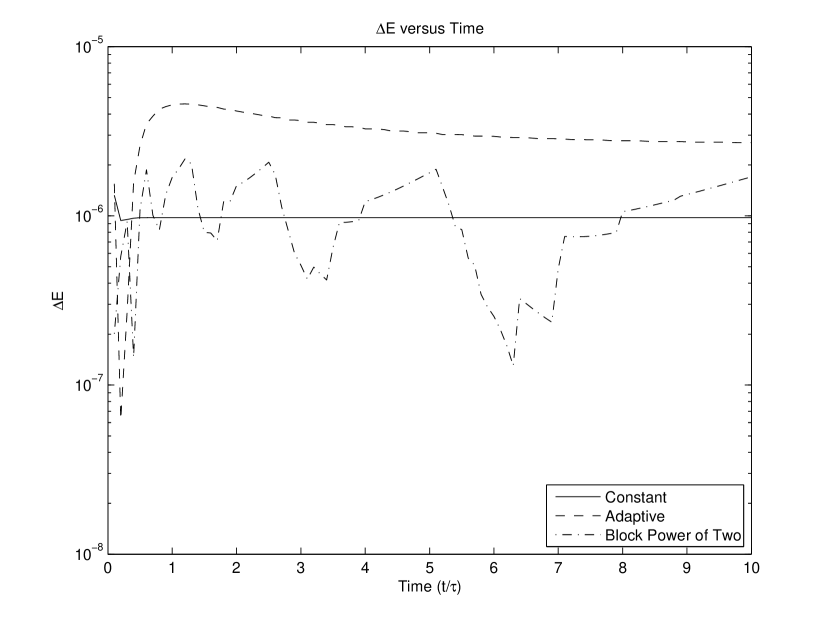
Figure 4: Relative energy error versus total evolution interval for simulations of the Kepler orbit described in the text. The orbital parameters are $a=2/45$, $e=9/10$, $E=-1/4$. The total evolution interval for each simulation varies from $0$ to $10\tau$ in steps of $\tau/10$. All three integration algorithms have comparable energy error.

Given an evolution mapping $F_{t}:(q,p)\mapsto(Q_{t}(q,p),P_{t}(q,p))$, the pushforward of the Poincaré integral invariant $\mathcal{I}\equiv dq\wedge dp$ along the trajectory $q(t),p(t)=F_{t}\left(q_{0},p_{0}\right)$ is given by

$$\left(F^{*}_{t}\mathcal{I}\right)\left(q_{0},p_{0}\right)=\left[\partial_{0}Q_{t}\left(q_{0},p_{0}\right)\partial_{1}P_{t}\left(q_{0},p_{0}\right)-\partial_{1}Q_{t}\left(q_{0},p_{0}\right)\partial_{0}P_{t}\left(q_{0},p_{0}\right)\right]dq_{0}\wedge dp_{0}.$$ (40)

All three integration algorithms are evolution mappings. An elegant algorithm (Sussman, 2006; Sussman et al., 2001) exists to compute derivatives of arbitrary computations, such as our evolution mappings, without the truncation error which would result from finite differencing. We used this algorithm to compute $\Delta I\equiv\left[\left(F^{*}_{t}\mathcal{I}\right)-\mathcal{I}\right]\left(q_{0},p_{0}\right)$ using equation (40). $\Delta I$ is a two form, and in a two-dimensional phase space it can be written $\Delta I=f(t)dq_{0}\wedge dp_{0}$, where $f$ is a scalar. The value of $f$ is plotted versus $t$ for the three algorithms in Figure 5. It is clear that the ordinary adaptive stepsize integrator does not conserve the symplectic form while the block-power-of-two and constant stepsize integrators do, as expected from Section 4. As explained in Section 4, though the energy error performance of the three algorithms is comparable, only the constant-timestep and block-power-of-two schemes are symplectic, and only the block-power-of-two scheme is symplectic and allows for adaptive timesteps.

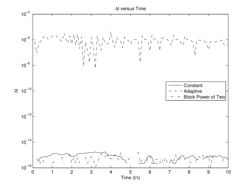
Figure 5: Error in the Poincaré integral invariant versus total evolution interval for the simulations of the Kepler orbit shown in Figure 4. The constant timestep (solid line) and block-power-of-two timestep (dot-dashed line) algorithms conserve the Poincaré integral invariant exactly while the adaptive timestep algorithm (dashed line) doesn’t, even though the energy error behaviors of the algorithms are comparable.

7.2 Many-Body Simulations

In this subsection we report on the application of the individual and adaptive timestep integration algorithm described in this paper to simulations of many-body systems. We choose to use the so-called “standard units”: units in which the total system mass $M=1$, $G=1$, and the total energy $E=-1/4$ (Heggie & Mathieu, 1986). In standard units, the virial radius of the system is 1. Our initial conditions are a randomly sampled Plummer model shifted into a coordinate system where the center of mass is at the origin and the total linear momentum is zero.

Because our code makes no special provision for close encounters, we used a softened gravitational potential:

$$V(r)=\frac{1}{\sqrt{r^{2}+\epsilon^{2}}},$$ (41)

with $\epsilon=4/N$, where $N$ is the number of bodies in a particular simulation. This is a standard technique in codes which do not carefully regularize the singular two-body potential (Aarseth, 2001).

7.2.1 Symplecticity Tests

An $N$-body system with $N$ bodies has a $6N$-dimensional phase space. Given an integration mapping, with Jacobian matrix $J$, conservation of the Poincaré integral invariant by the mapping implies that

$$S=J^{T}SJ,$$ (42)

where $S$ is the “symplectic unit”:

$$S=\left[\begin{array}[]{cc}0&-1\\ 1&0\end{array}\right]$$ (43)

where $1$ represents the identity matrix in $3N$-dimensions. Using a generalization of the algorithm for explicitly computing derivatives of computational algorithms, we can compute the Jacobian matrix for the evolution mapping defined by any integration scheme.

We denote by $dI$ the relative change in the sum of the absolute values of the diagonal from lower left to upper right between $J^{T}SJ$ and $S$. If equation (42) holds, $dI=0$. We compare $dI$ from the individual and adaptive timestep integrator described in this paper to $dI$ from a standard individual and adaptive timestep Hermite integrator (Makino, 1991). It is difficult to precisely control the stepsizes chosen in an adaptive timestep scheme, so we measure $dI$ as a function of the total number of steps taken for the evolution, $n_{\rm{steps}}$. An error which scales as $h^{r}$ should scale as $n_{\rm{steps}}^{-r}$.

Based on the discussion in Section 2.1.2, we expect that $dI$ from the variational integrator will be fifth order (that is, it scales as $n_{\rm{steps}}^{-5}$), while $dI$ from the Hermite integrator will be fourth order (exactly the same order as the integrator’s trajectory error). Figure 6 demonstrates that this is exactly the case for simulations of a Plummer initial condition with $N=25$ bodies and varying numbers of steps over a total time interval of $T=1.0$ by both algorithms.

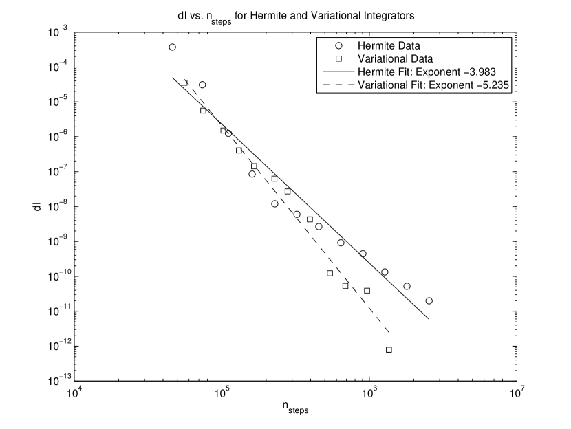
Figure 6: Error in equation (42) (non-conservation of the Poincaré integral invariant) in multiple integrations of $N=25$ Plummer initial conditions by the standard Hermite integrator and the individual and adaptive timestepping integrator described in the text over a total time interval of $T=1.0$ with various choices of (adaptive) timestep. The data have been least-squares fit to illustrate the scaling with $n_{\rm steps}$: the Hermite data fit with $dI\propto n_{\rm steps}^{-3.983}$, and the variational data fit with $dI\propto n_{\rm steps}^{-5.235}$, as expected from the discussion in Section 2.1.2.

Because they both depend on the accuracy of the solution to the implicit equation (16a), we expect that symplecticity and angular momentum conservation error would scale similarly in a long-term simulation. Results in the next section show that angular momentum error in a long-running simulation is about one order of magnitude better than the energy conservation error (Figure 7) using our algorithm, while the Hermite algorithm produces angular momentum errors commensurate with its energy conservation error. Our algorithm appears to have the advantage in angular momentum conservation and symplecticity in large-$N$, long-time simulations.

7.2.2 1000-body Cluster Simulation

Here we compare a 1000-body cluster simulation run using our variational integrator with another such simulation using the NBODY2h code (Aarseth, 2001). NBODY2h is not the state-of-the-art in cluster simulations; it is an appropriate comparison to our code because it uses the state-of-the-art Hermite integration algorithm but uses softening instead of treating close encounters specially. We have run many such simulations—the one described here is typical. Recall we use the standard units: the total system mass is $M=1$, $G=1$, and the total energy $E=-1/4$ (Heggie & Mathieu, 1986). In standard units, the virial radius of the system is 1. Initial conditions for both runs are a randomly sampled Plummer model shifted into a coordinate system where the center of mass is at the origin and the total linear momentum is zero. The random sampling differs between the two codes, so the initial conditions are not identical.

In the simulation reported here, we chose to keep energy conservation to better than a part in $5\times 10^{-9}$ per unit timestep, with a target of one part in $10^{-9}$. If, at the end of an advancement by $\Delta t=1.0$, the relative energy error was greater than $5\times 10^{-9}$ we re-started the step with a smaller $\eta$ parameter (cf. eq. (37)); at the end of every unit time interval, we adjusted $\eta$ according to

$$\eta^{\prime}=\eta\frac{10^{-9}}{\Delta E/E}.$$ (44)

A similar procedure is used to adjust the timestep in NBODY2h.

Figure 7 shows the time-evolution of the relative energy error and relative angular momentum error in the variational simulation. We can see in Figure 7 that the angular momentum conservation error is about an order of magnitude smaller than the energy conservation error. This is consistent with the fact that the angular momentum error scales one power of $h$ better than the energy error.

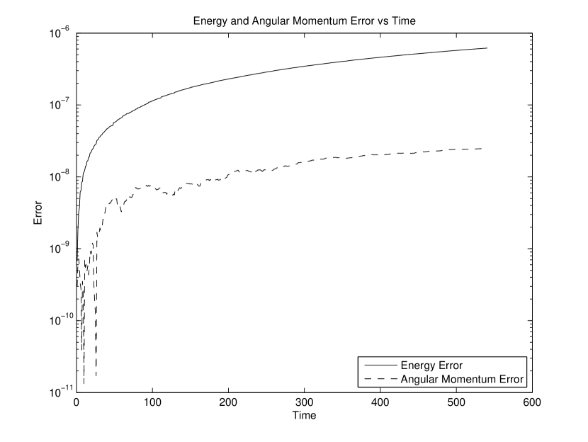
Figure 7: Relative energy and angular momentum conservation error for the 1000-body simulation performed using the variational integrator. As expected, the angular momentum conservation error is much better than the energy conservation error.

Figure 8 compares the core radius (computed as described in Casertano & Hut (1985)) versus time for the variational simulation with the core radius output by the NBODY2h simulation (recall that the two simulations do not start with identical initial conditions, but rather random samplings of identical phase-space distributions). The dynamical behavior of the core radius simulated using our algorithm is qualitatively correct. The NBODY2h simulation has momentum (both linear and angular) conservation error which is approximately commensurate with its energy conservation error—about one order of magnitude worse than the variational algorithm’s angular momentum conservation error, and six orders of magnitude worse than its linear momentum conservation error. Its wall-clock time is significantly better than the variational algorithm because our algorithm does not implement the nearest-neighbor scheme of Ahmad & Cohen (1973), and therefore evaluates all 999 potentials involving the body with the smallest timestep every step, all other 998 potentials involving the body with the second-smallest timestep every step for that body, etc.

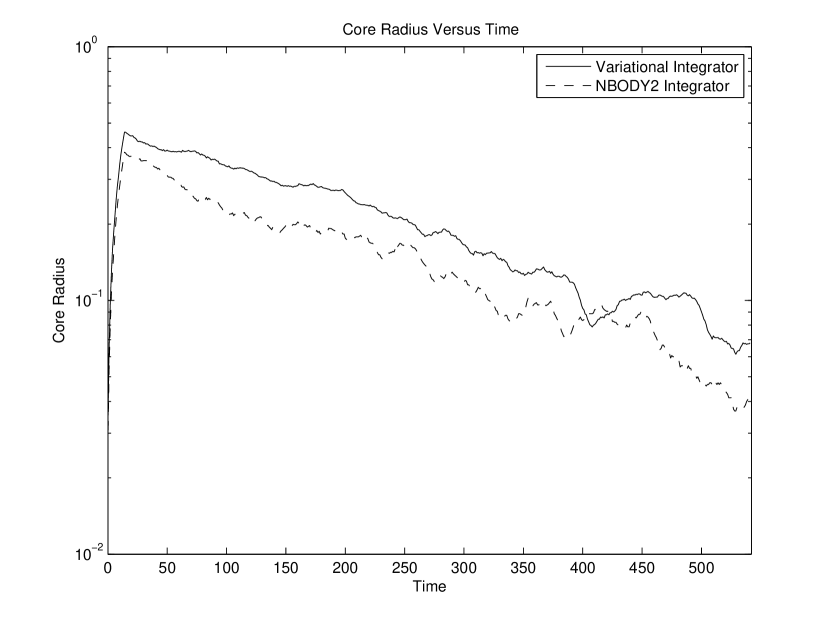
Figure 8: Core radius versus time for the simulation described in the text using the integrator in this paper and an equivalent simulation using the NBODY2h code. Boxcar averaging has been employed with $\Delta t=15$ to reduce fluctuations in the curves.

8 Discussion

We have presented a class of $N$-body integrators obtained by discretizing the action as opposed to discretizing the equations of motion. Such integrators automatically conserve discrete momenta and are symplectic. This paper focuses on the fourth-order, three-point GGL integrator described in Section 2.1.2, but Section 2 describes a general framework for constructing such integrators. We have demonstrated, theoretically in Section 4 and experimentally in Section 7.1, that adaptive timestepping integrators can still be symplectic if they use a block-power-of-two scheme. Individual timesteps (Section 5) impose requirements that reduce the symplecticity and angular momentum conservation from exact to fifth-order (one order better than the trajectory error of our integrator); nevertheless, we have shown experimentally in Sections 7.2.1 and 7.2.2 that the benefits of fifth-order symplecticity and angular momentum conservation are significant.

Though our code is not CPU-time competitive with standard stellar-cluster simulations due to their use of the Ahmad-Cohen nearest-neighbor scheme, we expect it will be useful in direct-summation $N$-body simulations where phase space volume conservation is more important than raw speed — though it would be interesting to see whether the Ahmad-Cohen scheme significantly affects the symplecticity of our algorithm in practice, we have not investigated this. We intend to use our algorithm to check the accuracy of dark matter halo evolution in larger, cosmological $N$-body simulations, and to investigate the formation of caustics in dark-matter distributions on a smaller scale. In these applications symplecticity is essential because the “coldness” of the dark matter phase-space distribution is fundamental to the dynamics.

Additionally, the algorithm was designed with the application to full cosmological $N$-body simulations in mind. The original motivation for the work was to find a higher-order, symplectic algorithm which takes only forward steps as an alternative to the leapfrog algorithm used in cosmological simulations. Standard compositional higher-order symplectic integrators are not useful in this context because the simulations of gas dynamics in high-accuracy cosmological simulations become unstable under evolution backward in time, and these integrators all have backwards timesteps. We intend to explore this application in a future paper.

References

- Aarseth (2001) Aarseth, S. J. 2001, New Astronomy, 6, 277
- Abramowitz & Stegun (1972) Abramowitz, M. & Stegun, I. A., eds. 1972, Handbook of Mathematical Functions, With Formulas, Graphs and Mathemacial Tables (Dover Publications, Inc.)
- Ahmad & Cohen (1973) Ahmad, A. & Cohen, L. 1973, Journal of Computational Physics, 12, 389
- Casertano & Hut (1985) Casertano, S. & Hut, P. 1985, ApJ, 298, 80
- Chambers (2003) Chambers, J. E. 2003, AJ, 126, 1119
- Chin & Chen (2005) Chin, S. A. & Chen, C. R. 2005, Celestial Mechanics and Dynamical Astronomy, 91, 301
- Ge & Marsden (1988) Ge, Z. & Marsden, J. E. 1988, Physics Letters A, 133, 134
- Heggie & Hut (2003) Heggie, D. & Hut, P. 2003, The Gravitational Million-Body Problem (Cambridge University Press)
- Heggie & Mathieu (1986) Heggie, D. & Mathieu, R. 1986, in The Use of Supercomputers in Stellar Dynamics, ed. S. McMillan & P. Hut (Springer), 233
- Lew et al. (2004) Lew, A., Marsden, J. E., Ortiz, M., & West, M. 2004, Int. J. Numer. Meth. Engng, 60, 153
- Makino (1991) Makino, J. 1991, ApJ, 369, 200
- Makino et al. (1996) Makino, J., Hut, P., Kaplan, M., & Saygin, H. 1996, NewA, 12, 123
- Marsden & West (2001) Marsden, J. E. & West, M. 2001, Acta Numerica, 357
- Omelyan (2006) Omelyan, I. P. 2006, Physical Review E, 74
- Preto & Tremaine (1999) Preto, M. & Tremaine, S. 1999, AJ, 118, 2532
- Scuro & Chin (2005) Scuro, S. R. & Chin, S. A. 2005, Physical Review E, 71, 056703
- Sheng (1989) Sheng, Q. 1989, IMA Journal of Numerical Analysis, 9, 199
- Shirokov & Bertschinger (2005) Shirokov, A. & Bertschinger, E. 2005, astro-ph/0505087
- Springel (2005a) Springel, V. 2005a, private communication
- Springel (2005b) —. 2005b, Monthly Notices of the Royal Astronomical Society, 364, 1105
- Stuchi (2002) Stuchi, T. J. 2002, Brazillian Journal of Physics, 32, 958
- Suris (1989) Suris, Y. B. 1989, USSR Comput. Maths. Phys., 29, 138
- Sussman (2006) Sussman, G. J. 2006, private communication
- Sussman et al. (2001) Sussman, G. J., Wisdom, J., & Mayer, M. E. 2001, Structure and Interpretation of Classical Mechanics (The MIT Press)
- Suzuki (1991) Suzuki, M. 1991, Journal of Mathematical Physics, 32, 400
- Wisdom & Holman (1991) Wisdom, J. & Holman, M. 1991, The Astronomical Journal, 102, 1528
- Wisdom et al. (1996) Wisdom, J., Holman, M., & Touma, J. 1996, Fields Institute Communications, 10, 217
- Yoshida (1993) Yoshida, H. 1993, Celestial Mechanics and Dynamical Astronomy, 56, 27