MAXIPOL: Cosmic Microwave Background Polarimetry
Using a Rotating Half-Wave Plate

Abstract

We discuss MAXIPOL, a bolometric balloon-borne experiment designed to measure the E-mode polarization of the cosmic microwave background radiation (CMB). MAXIPOL is the first bolometric CMB experiment to observe the sky using rapid polarization modulation. To build MAXIPOL, the CMB temperature anisotropy experiment MAXIMA was retrofitted with a rotating half-wave plate and a stationary analyzer. We describe the instrument, the observations, the calibration and the reduction of data collected with twelve polarimeters operating at 140 GHz and with a FWHM beam size of 10 arcmin. We present maps of the $Q$ and $U$ Stokes parameters of an 8 deg² region of the sky near the star $\beta$-UMi. The power spectra computed from these maps give weak evidence for an $EE$ signal. The maximum-likelihood amplitude of $\ell(\ell+1)C^{EE}_{\ell}/2\pi$ is $55_{-45}^{+51}~{}\mu\mbox{K}^{2}$ (68%), and the likelihood function is asymmetric and skewed positive such that with a uniform prior the probability that the amplitude is positive is 96%. This result is consistent with the expected concordance $\Lambda$CDM amplitude of $14~{}\mu\mbox{K}^{2}$. The maximum likelihood amplitudes for $\ell(\ell+1)C^{BB}_{\ell}/2\pi$ and $\ell(\ell+1)C^{EB}_{\ell}/2\pi$ are $-31_{-19}^{+31}$ and $18_{-34}^{+27}~{}\mu\mbox{K}^{2}$ (68%), respectively, which are consistent with zero. All of the results are for one bin in the range $151\leq\ell\leq 693$. Tests revealed no residual systematic errors in the time or map domain. A comprehensive discussion of the analysis of the data is presented in a companion paper.

1 Introduction

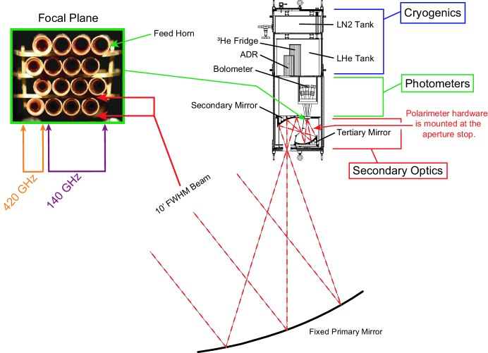
Figure 1: An overall view of the MAXIPOL instrument. Most of the elements shown here were shared with the previous MAXIMA experiment. The polarimeter hardware, which is not shown here, is shown in Figure 2.

Measurements of the polarization of the cosmic microwave background radiation (CMB) can confirm fundamental predictions made by our cosmological model and probe the period after the Big Bang when inflation is believed to have occurred. Several experiments recently reported detection of either the $TE$ or $EE$ power spectrum (Readhead et al., 2004; Barkats et al., 2005; Montroy et al., 2005; Leitch et al., 2005; Page et al., 2006) and there is on-going effort to build even more sensitive receivers that can probe the small signal amplitudes that are predicted for the $BB$ power spectrum.

MAXIPOL is a bolometric, balloon-borne experiment designed to measure the polarization of the CMB. It uses a rotating half-wave plate (HWP) and a wire grid analyzer to modulate signals reaching the bolometers from polarized sources. MAXIPOL is unique in that it is the only bolometric CMB experiment to date to deploy rapid polarization modulation. With our technique, the polarized component of the incident radiation is modulated at a frequency equal to four times the rotation frequency of the HWP. This property is advantageous for measuring the small CMB polarization because polarized sky signals are moved to a narrow band in the frequency domain which can be far from detector 1/$f$ noise or other spurious instrumental signals. In particular, there is no confusion with spurious signals that appear at the modulation frequency itself. Because only polarized signals are modulated, a HWP polarimeter separates the temperature and polarization signals in the frequency domain, making analysis of the signals independent. Of particular importance is the property that each detector is an independent polarimeter measuring the Stokes parameters $I$, $Q$, and $U$ over a relatively short time. Several systematic errors that complicate detector differencing techniques are avoided.

Differencing polarimeters are defined here as instruments that measure Stokes parameters by differencing the signal from two detectors, each of which is sensitive to one of the orthogonal linear polarizations. Differencing polarimeters can be constructed using individual polarizers placed at the entrance aperture of each photometer, two bolometers with orthogonal absorbing grids, or orthomode transducers which split the incoming polarization into two components (see for example Masi et al., 2006; Benoit et al., 2004). Differencing polarimeters only modulate polarized sky signals through sky rotation and telescope scanning. They are prone to spurious polarization signals through errors in the absolute calibration of detector pairs, time dependent responsivity variations, noise properties that are not common to both detectors, or different antenna patterns for the two detectors. Polarization modulators like the one used in MAXIPOL can mitigate these problems.

Polarization modulation technologies different from MAXIPOL’s include rotating polarizers, photoelastic modulators and Faraday rotation modulators. Rotating polarizers reflect the unwanted polarization component and can thus produce spurious signals through multiple reflections inside the receiver. Suitable photoelastic modulators have not been developed in the frequency bands of interest. Broadband Faraday rotation modulators for the millimeter-wave band are just now being developed (Yoon et al., 2006) and little is known about systematic errors associated with their operation. Modulation of sky signals with a rotating HWP and stationary analyzer is a proven technique in infrared and millimeter-wave astrophysics (Tinbergen, 1996) and therefore we chose to implement the technique for CMB polarimetry. Since MAXIPOL is the first CMB experiment to produce results using this strategy, the experience gained from hardware implementation, data analysis and characterization of HWP-specific systematic errors will inform the design of next-generation experiments that aim to characterize the anticipated B-mode signals.

To build MAXIPOL, the receiver from the CMB temperature anisotropy experiment MAXIMA (Hanany et al., 2000; Balbi et al., 2000; Lee et al., 2001; Stompor et al., 2001; Abroe et al., 2004) was converted into a polarimeter by retrofitting it with a HWP and a fixed polarization analyzer. The rest of the MAXIMA instrument including the detector system, cryogenics, optics, and electronics was essentially unchanged. MAXIPOL observed the sky during two flights that were launched from the NASA Columbia Scientific Ballooning Facility (CSBF) in Ft. Sumner, New Mexico. The first flight, launched in 2002 September, yielded less than an hour of useful data because of a telemetry failure. The primary CMB data set, which will be discussed in this paper, was collected during the second flight in 2003 May.

We describe the instrument and the observations in Sections 2 and 3. The HWP-specific information appears in Sections 4, 5, 6, and 8. In particular, Section 5 describes the processing of our time-domain data. This information will be useful for future CMB experiments that will use HWP polarimeters. Estimated power spectra and $Q$ and $U$ maps are presented in a summary of our analysis in Section 7. A comprehensive description of the analysis is given in Wu et al. (2006).

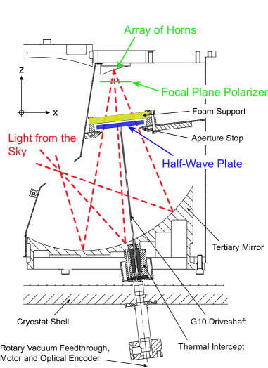
Figure 2: A cross-sectional view of the receiver near the focal plane showing the polarimetry components. The HWP was mounted at an aperture stop of the optical system and a roof-shaped polarization analyzer was mounted in front of the entrance apertures of the horns. A sketch showing the analyzer and the focal plane projected on a perpendicular plane is given in Figure 3.

2 Instrument

In this Section, we give an overview of the experiment emphasizing the polarimeter. Additional technical details are given in previous MAXIMA publications (Lee et al., 1998; Hanany et al., 2000; Rabii, 2002; Winant, 2003; Rabii et al., 2006) and MAXIPOL papers (Johnson et al., 2003; Johnson, 2004; Johnson et al., 2006; Collins, 2006).

MAXIPOL employed a three-mirror telescope with a 1.3 m off-axis parabolic primary mirror. The elliptical secondary and tertiary reimaging mirrors were maintained at liquid helium temperatures inside the receiver to reduce radiative loading on the bolometers. The primary mirror, which was nutated to produce rapid azimuth modulation for MAXIMA, was fixed for MAXIPOL to avoid modulating the polarization properties of the telescope.

Millimeter-wave radiation from the sky was re-imaged to a $4\times 4$ array of photometers at the focal plane. Observations were made in bands centered on 140 and 420 GHz with $\Delta\nu\simeq$ 30 GHz. The twelve 140 GHz photometers were optimized to measure the CMB and the four 420 GHz photometers were used to monitor foreground dust contamination. The 10^′ FWHM Gaussian beam shape for the 140 GHz photometers was defined by a smooth-walled, single-moded conical horn and a cold Lyot stop. The 420 GHz photometers employed multi-mode Winston horns. The bolometers were maintained at 100 mK by the combination of an adiabatic demagnetization refrigerator (Hagman & Richards, 1995) and a 300 mK ³He refrigerator. A photograph of the focal plane and a cross-sectional overview of the optical system, which was essentially unchanged from MAXIMA, are shown in Figure 1.

Figure 2 shows a cross-section of the portion of the cold optics that was modified to convert MAXIMA to MAXIPOL. We used a 3.175 mm thick A-cut sapphire HWP. Reflections from the HWP were minimized by bonding 330 $\mu$m thick wafers of Herasil to each face of the sapphire with Eccobond 24, an unfilled, low viscosity epoxy that was used to achieve glue layers as thin as 13 $\mu$m. The HWP thickness was selected to minimize the fraction of emerging elliptically polarized intensity and thereby optimize the overall modulation efficiency of the polarimeter. The calculated efficiency incorporated the effects of the finite spectral bandwidth of the photometers and the oblique incidence of rays on the HWP.

Since the anti-reflection coating was not birefringent, the two incident polarization orientations had different coefficients of reflection. This differential reflection gave rise to a HWP synchronous signal at a frequency of $2f_{o}$, where $f_{o}$ is the rotation frequency of the HWP. To minimize this effect, we calculated the anti-reflection coating thickness that would minimize the difference in reflection coefficients given the spectral bandwidth of the 140 GHz photometers, the thickness of the Eccobond 24 layer and the angles of the rays. The $2f_{o}$ signal was not a source of systematic error because it was out of the polarization signal band centered on $4f_{o}$ (see Section 5).

The polarization analyzer was a commercial grid polarizer epoxied to a rigid “roof-shaped” frame that was positioned over the horn openings (see Figure 3). This roof-shaped polarizer was implemented so that the light that was reflected by the grid was directed out of the optical path and into a cold millimeter-wave absorber (Bock, 1994) that was mounted on both sides of the focal plane. The grid polarizer had 98 electroformed gold stripes per cm that were bonded onto a 38 $\mu$m thick Mylar substrate. The stripes were 5 $\mu$m wide.

Figure 3: A sketch of the roof-shaped analyzer positioned in front of the array of horns at the focal plane.

The HWP was located near the Lyot stop and was driven from its axis at $f_{o}$ = 1.86 Hz during all observations (see Figure 2). The orientation of the HWP was measured with a 17-bit optical encoder. This rotation frequency, combined with the azimuth scan frequency that was either 0.10 Hz or 0.06 Hz during the primary CMB observations, gave approximately three to five modulations of the $Q$ and $U$ Stokes parameters per 10 arcmin sky beam in one azimuthal scan.

3 Observations and Scans

The instrument was launched at 15:14 UT (9:14 AM Local Time) on 2003 May 24. The first observation began at 18:08 UT when the payload reached an altitude of 38.7 km. The flight terminated 26 hours after launch, 477 km west and 120 km south of the launch site. In this paper we only discuss the data collected during one 7.6 hour-long nighttime CMB observation near Beta Ursae Minoris ($\beta$-UMi), RA = 14h 50^′ 42.5^′′, Dec= +74^∘ 09^′ 42.^′′ Other observations are discussed in Johnson (2004) and Collins (2006).

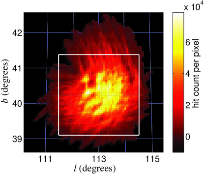
Figure 4: Map of the total number samples per 3^′ pixel from the twelve 140 GHz polarimeters for the $\beta$-UMi observation. The white square marks the $2.3^{\circ}\times 2.3^{\circ}$ region used for power spectrum estimation.

Jupiter was observed during both the day and nighttime portions of this flight to obtain the absolute intensity calibration of the instrument, to map the telescope beam shapes, and to measure the location of the beam centers for pointing reconstruction. During these observations the gondola was scanned in azimuth with a triangle-wave profile centered on Jupiter. The turnarounds on this profile were smoothed to ensure quiescent noise performance from the bolometers. The daytime scans were $\pm 0.6^{\circ}$ with a 20 sec period. The nighttime scans were $\pm 1.3^{\circ}$ with an 18 sec period. Simultaneously, the telescope elevation was rastered $\pm 0.5^{\circ}$ relative to the planet every 20 min.

For the CMB observations the telescope azimuth was scanned in a similar fashion near $\beta$-UMi, but with an amplitude of $1^{\circ}$ and a period that was changed mid-scan from 10 to 15 sec. To improve cross-linking the telescope elevation was re-pointed $0.2^{\circ}$ above and below the guide star every 10 min. Figure 4 shows the total number of 140 GHz detector samples per 3 arcmin pixel produced by this scan strategy. Observation statistics including pointing error for all scans are given in Table 1.

			Pointing Error
Scan Target	Start Time	Duration	Random	Systematic
	[UT]	[hours]	[arcmin]	[arcmin]
Daytime Jupiter	20:03	1.02	0.99	0.31
Nighttime Jupiter	02:42	0.52	0.47	0.21
$\beta$-UMi	03:18	7.64	0.32	0.27

Table 1: Scan targets with scan durations and pointing error. A detailed description of the pointing errors is given in Collins (2006).

4 Attitude Reconstruction

Telescope pointing was primarily determined with one of two star cameras. The camera used during daytime observations was filtered with a 695 nm Schott glass filter to reduce the brightness of the daytime sky, and fitted with a reflective lens that had a 500 mm focal length, which provided a FOV of 0.72^∘ by 0.55^∘. The unfiltered nighttime camera used a 50 mm lens that provided a 7.17^∘ by 5.50^∘ FOV. Pointing reconstruction using star camera data has been described in previous publications (Hanany et al., 2000; Rabii, 2002; Rabii et al., 2006; Collins, 2006).

MAXIPOL adopts the convention for the Stokes parameters $I$, $Q$, and $U$ used by WMAP, which references the polarization direction to the NGP (Hinshaw et al., 2003; Zaldarriaga & Seljak, 1997). When the instrument observes pixel $p$ at time $t$, the output of the detectors (in units of volts and ignoring noise and systematic errors that will be discussed later) can be written

$$d_{p}(t)=R\,[\,I_{p}\!\!\!\! + \!\!\!\!\epsilon\,Q_{p}\,\cos\left(\,2\gamma(t)\,\right)$$ (1)

$$+ \!\!\!\!\epsilon\,U_{p}\,\sin\left(\,2\gamma(t)\,\right)\,].$$

Here $\gamma$ is the angle between the polarization reference vector at sky pixel $p$ and the polarimeter transmission axis, $\epsilon$ is the polarimeter modulation efficiency, and $R$ is an overall calibration factor that has units of V K^-1 (Collins, 2006). The angle $\gamma$ is given by

$$\gamma=\alpha-2\beta-\frac{\pi}{2}.$$ (2)

Here, $\alpha$ is the angle between the reference vector at pixel $p$ and a vector pointing from $p$ to the zenith along a great circle, $\beta$ is the HWP orientation angle in the instrument frame, and the $\pi/2$ accounts for the fact that the transmission axis of the analyzer was perpendicular to the zenith axis. The angle $\alpha$ was computed for each time sample from the pointing reconstruction. The angle $\beta$ was computed by subtracting a photometer-dependent offset from the HWP encoder angle. This encoder offset was measured during laboratory calibration (see Section 6.2). By combining Equations 1 and 2 the model for noiseless time ordered data (TOD) can be written

$$d(t)=R\,[\,I_{p}\!\!\!\! - \!\!\!\!\epsilon\,Q_{p}\,\cos(\,4\beta(t)-2\alpha(t)\,)$$ (3)

$$+ \!\!\!\!\epsilon\,U_{p}\,\sin(\,4\beta(t)-2\alpha(t)\,)\,].$$

5 Time Ordered Data Processing

In this paper we report on the data from the twelve 140 GHz polarimeters. The raw data from $\beta$-UMi consists of 5.76 million time-ordered samples for each of the 140 GHz polarimeters. The bolometer sample period was 4.8 msec. We first give an overview of the time-domain data-processing algorithm, which is outlined in Figure 5, and then discuss some of the processing steps in more detail. The rest of the data analysis procedure is described in the companion paper, Wu et al. (2006).

Transients such as cosmic ray hits and internal calibration pulses were flagged using an algorithm described in Johnson (2004). The data were calibrated and blocks of data separated by gaps longer than 30 sec were processed as separate segments. These time domain data contained a significant instrumental signal that was synchronous with the rotation of the HWP. We refer to this instrumental signal as the HWP synchronous signal (or sometimes in short the synchronous signal). An initial estimate of the synchronous signal was subtracted. Gaps shorter than 30 sec were filled with constrained noise realizations, and the synchronous signal was replaced, leaving continuous, transient-free data. The instrumental filters were deconvolved after padding the ends of each segment with 100 msec of matched white noise, simulated HWP synchronous signal, and a window function that smoothly decayed to zero at the endpoints. A section of data one filter-time-width long was removed from the ends of each data segment after filter deconvolution to avoid any contamination from edge effects produced by the Fourier transforms. The HWP synchronous signal was then re-estimated and subtracted from the raw data, producing the time-ordered data (TOD). The time-ordered polarization data (TOPD) were extracted from the TOD by demodulation using a phase-locked, sine-wave reference signal constructed from the angle $2\gamma$. The TOPD were checked for noise stationarity using a frequency-domain $\chi^{2}$ test and for Gaussianity using the Kolmogorov-Smirnoff (KS) test in the time domain.

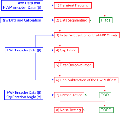
Figure 5: A flowchart of the time-domain processing algorithm. Blue boxes at left are data inputs, numbered red boxes in the middle are analysis operations and green boxes at right are data outputs.

The following subsections describe the details of the HWP synchronous signal estimation, the filter deconvolution, the TOPD demodulation, and the tests of the noise properties.

5.1 Subtraction of the HWP Synchronous Signal

$\begin{array}[]{cc}\includegraphics[height=187.90244pt,angle={90}]{./f6a.eps}&\includegraphics[height=187.90244pt,angle={90}]{./f6b.eps}\\ (a)&(b)\\ \includegraphics[height=187.90244pt,angle={90}]{./f6c.eps}&\includegraphics[height=187.90244pt,angle={90}]{./f6d.eps}\\ (c)&(d)\\ \end{array}$

Figure 6: $(a)$ A 16 min long sample of raw data from one 140 GHz polarimeter plotted versus the HWP angle $\beta$. $(b)$ Power spectrum of the raw data. $(c)$ Power spectrum of the data after subtraction of the HWP synchronous signal (TOD). $(d)$ Power spectrum of the demodulated TOD, which is the TOPD. Zero-frequency in $(d)$ is $4f_{o}$ in $(b)$ and $(c)$. The red, dashed curves in panels $(b)$, $(c)$ and $(d)$ mark the polarization signal bands limited by the telescope scan frequency and the beam. The blue, dash dot curves in panels $(b)$ and $(c)$ mark the temperature signal band. Some 1/$f$ noise appears in the temperature band.

The raw data were dominated by the HWP synchronous signal, which came from thermal emission from the HWP drivetrain, differential transmittance from the HWP, and modulated instrumental polarization. Emission from the HWP drivetrain appeared at harmonics of $f_{o}$ with power which decreased with frequency. Differential transmittance contributed primarily at $2f_{o}$, and polarized signals generated by instrumental polarization were dominant at $4f_{o}$.

We modeled the synchronous signal as a sum of $n=8$ harmonics of the HWP rotation frequency with amplitudes $\xi_{n}$ and phases $\chi_{n}$

$$\mbox{HWPSS}\left(t\right)=\sum_{n=1}^{8}\xi_{n}(t)\,\sin\left(\,n\beta(t)+\chi_{n}(t)\,\right)$$ (4)

where HWPSS is the synchronous signal. Recall that $\beta(t)$ is the HWP rotation angle in the instrument frame. We used only eight harmonics because signals at higher frequencies were blocked by the filters discussed in Section 5.2. Each of the three sources listed above (thermal emission, differential transmission, and instrumental polarization) contributed its own amplitude and phase to produce the net amplitude $\xi$ and phase $\chi$ in each of the harmonics. We allowed the amplitude of each of the three sources to change linearly with time but we fixed their phase angles relative to the instrument frame. Thus the contribution of the $n$th harmonic of the synchronous signal can be written as

$$\mbox{HWPSS}_{n}(t)=\xi_{n}(t)\,\sin\left(\,n\beta(t)+\chi_{n}(t)\,\right)$$

$$=\sum_{j=1}^{3}\left(A_{nj}+B_{nj}t\right)\,\sin\left(\,n\beta(t)+\phi_{nj}\,\right)$$ (5)

where $A_{nj}$, $B_{nj}$, and $\phi_{nj}$ are constants. Trigonometric identities can be used to relate Equations 4 and 5 and to rewrite the synchronous signal as

$$\mbox{HWPSS}(t)=\sum_{n=1}^{8}\!\!\!\!\! (\,C_{1n}+C_{2n}t\,) \!\!\!\!\cos\left(\,n\beta(t)\,\right)$$

$$+\!\!\!\!\! (\,S_{1n}+S_{2n}t\,) \!\!\!\!\sin\left(\,n\beta(t)\,\right)$$ (6)

with appropriate relations between $\xi$, $\chi$, $A$, $B$ and the constants $C_{1n}$, $C_{2n}$, $S_{1n}$, and $S_{2n}$. We subtracted the HWP synchronous signal from the raw time domain data using fits to Equation 6 in the following way.

The 32 $C$ and $S$ coefficients were assumed to be constant within each data segment and were estimated in each segment by an iterative demodulation procedure. To begin the first iteration, the data segment was demodulated for $n=1$ with the reference signal $\cos(\beta)$. The coefficients $C_{11}$ and $C_{21}$ were estimated using a linear least-squares fit to the output, ignoring the flagged data contaminated with transients. The component corresponding to $C_{11}$ and $C_{21}$ was constructed and subtracted from the data. The subtraction was repeated with the $\sin(\beta)$ reference signal, and then for the harmonics $n=2,...,8$ in order. The process was then iterated 25 times. After each iteration the new estimates of $C$ and $S$ were added to the old estimates. For a typical photometer, after four iterations of this process the difference between the data and the HWP synchronous signal was observed to be indistinguishable from random noise (see Section 5.1.1).

The amplitude values ranged from approximately 1.5 to 106 mK for harmonic $n=1$, from 30 to 250 mK for $n$ =2, and from 33 to 600 mK for $n=4$. The amplitude drifts were typically 0.5% over a 10 min data segment and 10% over a 3 hour time scale. The phases $\chi_{n}$ typically varied by less than 5 deg over the entire CMB scan. More details about the characterization of the HWP synchronous signal are given in Collins (2006).

Figure 6 shows the properties of one segment of data from one of the polarimeters before and after subtraction of the synchronous signal. Panel $(c)$ shows that the power spectrum of the data after the synchronous signal was subtracted is flat in the vicinity of $4f_{0}=7.4$ Hz and also down to frequencies well below 1 Hz. This white-noise level is the nominal noise level of the instrument.

The subtraction of the synchronous signal was tested using several figures of merit which address the following questions. Are the data after subtraction Gaussian distributed? Does the subtraction of the synchronous signal remove CMB signal from the map? Are there residuals of the synchronous signal in the map domain? How stable is the $4f_{0}$ component of the synchronous signal  and is it well-fit by the slow time variation of the model? We will address the first three questions here and the others in Section 5.3.

5.1.1 Gaussianity

The properties of the data after the HWP synchronous signal was subtracted were tested by band-pass filtering the TOD between 0.3 and 8.9 Hz to select the band that contains the first four Fourier modes of the synchronous signal. The data were decorrelated by filling the rejection band with a white noise realization, and then averaged into 36 bins in the HWP angle domain, each spaced by $10^{\circ}$. The $10^{\circ}$ bin size was selected so any residual $4f_{o}$ signal could be resolved. A $\chi^{2}$ statistic was calculated over the 36 bins for each data segment to search for residual HWP synchronous signal. The set of $\chi^{2}$ from each polarimeter was compared to the $\chi^{2}$ distribution for 36 independent degrees of freedom using the KS test, and no excess was found.

5.1.2 Removal of CMB Signal

We simulated the removal of the HWP synchronous signal with simulated raw time streams that had the same properties as our real time streams. The synchronous signal, the pointing information, and the noise estimate from each segment of data were used with simulated CMB polarization maps to assemble a simulated raw data stream composed of the synchronous signal, the HWP-modulated CMB polarization signal, and a noise realization with a power spectrum given by Equation 9. The subtraction of the synchronous signal was performed on each segment, the noise was subtracted, and the CMB signal was recovered by demodulation (see Section 5.3). The initial CMB TOPD was subtracted from the final. The residuals were bandpass filtered between 0.05 and 1.5 Hz, and then averaged into maps of $3^{\prime}$ pixelization using weights set by the noise level in each segment. In the $2.3^{\circ}\times 2.3^{\circ}$ square region used in the power spectral analysis the residual maps had an RMS of $0.018\pm 0.002\mu$K in $Q$ and $0.016\pm 0.001\mu$K in $U$ over five trials. These residuals were negligible compared to the RMS of simulated CMB maps of the same region, which was 4 $\mu$K for both $Q$ and $U$.

5.2 Filter Deconvolution

Photometer	$NEQ,U$	Modulation	$\tau_{A}$, $\tau_{B}$	$W_{A}$, $W_{B}$	Calibration	FWHM
	$\mu\mbox{K}\sqrt{\mbox{sec}}$	Efficiency	[ms]	[weight]	$\times 10^{-5}$ [V K-1]	[arcmin]
b13	780	0.92	5, 27	0.78, 0.22	2.30	9.2,	10.2
b14	2000	0.93	11, 41	0.55, 0.45	1.56	9.8,	9.9
b15	1100	0.90	8, 29	0.64, 0.36	2.32	9.3,	10.8
b23	780	0.93	8, 41	0.66, 0.34	2.18	10.0,	11.1
b24	870	0.93	8, 50	0.28, 0.72	3.32	10.2,	11.3
b25	710	0.93	10, 56	0.44, 0.56	2.91	10.3,	10.7
b33	1000	0.93	9, 46	0.50, 0.50	2.15	9.4,	10.4
b34	910	0.93	8, 26	0.39, 0.61	1.98	9.3,	10.6
b35	880	0.94	12, 64	0.49, 0.51	2.34	9.5,	10.6
b43	1200	0.95	9, 46	0.50, 0.50	1.93	8.6,	11.3
b44	1700	0.93	11, 74	0.38, 0.62	1.90	9.0,	11.4
b45	1100	0.92	14, 57	0.42, 0.58	2.42	9.8,	12.1
receiver	280	0.93	9, 46	0.50, 0.50	2.28	9.5,	10.9

Table 2: Characteristics of each of the 140 GHz polarimeters in the array. The row labeled “receiver” contains the inverse square sum of all $NEQ,U$ values thereby giving the total receiver performance. Other elements in this row are simple averages. The two bolometer time constants, $\tau_{A}$ and $\tau_{B}$, and their corresponding weights, $W_{A}$ and $W_{B}$, are differentiated with the subscripts $A$ and $B$. Typical beam FWHM uncertainties from the MCMC analysis are 2%, while typical calibration and modulation efficiency uncertainties are 13% and 2%, respectively. The $NEQ,U$ and the calibration are consistent with an instrument model that includes the bolometer noise, the amplifier noise, the measured bolometer time constants, the transmission of the analyzer, and the reflectance of the HWP.

The TOD were filtered in the readout electronics with high- and low-pass Butterworth filters with edges at approximately 15 mHz and 20 Hz, respectively. In addition, the frequency response of the bolometers attenuated and phase-delayed the modulated $4f_{o}$ signals at 7.4 Hz by about 35% and $20^{\circ}$ of HWP angle, respectively. The frequency response of the bolometers was measured in the laboratory. The results were modeled with two time constants and the parameters are shown in Table 2. Alternative analysis methods gave somewhat different parameters for the values of the time constants and of the relative weights. These differences were larger than the errors on the parameters within any given method. However, calculations showed that the differences between any of the derived filter functions in terms of amplitude and phase response at the signal band-width near 7.4 Hz were small such that the effect on the final results would have been negligible compared to the calibration uncertainty or to the uncertainty on mixing between the E and B modes due to noise.

The effects of the electronic filters and bolometer time constants were removed from the TOD by deconvolving the complex filter $\mathcal{F}$, where

$$\mathcal{F}(f)=\mathcal{F}_{hp}\mathcal{F}_{lp}\mathcal{F}_{bolo}/|\mathcal{F}_{lp30}|.$$ (7)

Here, $\mathcal{F}_{hp}$ and $\mathcal{F}_{lp}$ are the electronic high and low-pass filters, $\mathcal{F}_{bolo}$ is the bolometer response function, and $|\mathcal{F}_{lp30}|$ is a real, phase-preserving software filter with a low-pass cutoff of 30 Hz. This filter was included to suppress the spurious high frequency noise created by the deconvolution of the bolometer response function.

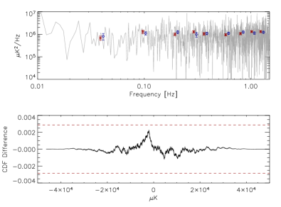
Figure 7: Top panel: The power spectrum of a 12.4 min long segment of TOPD for $Q$ with the binned power spectra of the first and second halves overplotted (red stars and blue diamonds). The binned power spectra are slightly offset in frequency from the bin center for clarity. This segment was deemed stationary by the stationarity test, with $\chi^{2}=12.52$ for 9 degrees of freedom. The cutoff $\chi^{2}$ for stationarity for the 12.4 min long chunk length was 19.43 (see Section 5.4). Bottom panel: the difference between the cumulative distribution function (CDF) of decorrelated $Q$ data from one data segment and the CDF of a Gaussian distribution of the same standard deviation. The KS statistic showed no non-Gaussianity above the 0.26$\sigma$ level for this segment. The red dashed lines mark the 1$\sigma$ significance level.

5.3 Demodulation

Modulation by the rotating HWP, combined with telescope scanning, moves the polarized sky signals to sidebands of $4f_{o}$, as shown in Figure 6. To extract the $Q$ and $U$ sky signals we used a software lock-in technique. The TOD were demodulated with the reference signals $-\cos(4\beta-2\alpha)/\epsilon$ and $\sin(4\beta-2\alpha)/\epsilon$ to produce the $Q$ and $U$ TOPD, respectively. Demodulated polarized sky signals lie in a band defined at the low frequency side by the $\sim$0.06 Hz telescope scan frequency and at the high side by attenuation from the beam above approximately 1.5 Hz, see Figure 6. For map making, the demodulation procedure also included a band-pass filter with high and low-pass edges at 0.05 and 1.5 Hz, respectively, that was used to reject any out-of-band signals.

Figure 6$(d)$ shows the power spectrum of one segment of $Q$ TOPD. This power spectrum is flat down to a frequency of approximately 1 mHz. The flatness is a measure of the degree of stability of the $4f_{o}$ component of the HWP synchronous signal and the efficacy of the subtraction method. For 99.5% of the TOPD from all photometers the $1/f$ knee was below 0.06 Hz.

5.4 Noise Characterization

The TOPD were checked for stationarity by bisecting each data segment and comparing the power spectra of the two halves. For this comparison, the portion of the power spectra that spanned the polarization signal band between 0.02 and 1.5 Hz was divided into nine bins. This choice of binning gave at least 8 frequency modes per bin for the shortest data segments, which were approximately 2 min long. The following $\chi^{2}$ statistic

$$\chi^{2}=\sum_{i=1}^{9}\frac{(P_{1i}-P_{2i})^{2}}{\sigma_{1i}^{2}+\sigma_{2i}^{2}}$$ (8)

was used to assess the similarity of the power spectra. Here, the sum extends over the nine bins, and $P_{i}$ and $\sigma_{i}$ were the mean and standard error of the power spectrum in each bin, respectively. The distribution of this statistic for white noise time streams was estimated with Monte-Carlo simulations of 20,000 realizations. Seven different segment lengths ranging from 2 to 24 min were considered. The range of segment lengths were selected based on the maximum and minimum lengths of the data segments used for map making. The $\chi^{2}$ corresponding to the probability to exceed $2\sigma$ was stable to 3% over this range of segment lengths and was estimated for an arbitrary segment length by spline-interpolating the $2\sigma$ $\chi^{2}$ between the seven simulated lengths.

The criterion of 2$\sigma$ stationarity was used with an algorithm that searched for long sub-segments of stationary data. A routine recursively cut each data segment into two halves if the two power spectra were dissimilar. After bisection, an iterative routine attempted to concatenate adjacent sub-segments whose power spectra were not yet known to be dissimilar. The sub-segment was flagged as non-stationary if the sub-segment length after this procedure was less than 2 min. Non-stationarity was mostly confined to three of the twelve 140 GHz photometers for which approximately 11% of the TOPD were discarded as non-stationary. The average stationary sub-segment length was 9 min. The upper panel of Figure 7 shows an example of a segment of data that was found to be stationary.

To quantify any $1/f$ noise in the TOPD the following three parameter model

$$P(f)=\sigma_{w}\left[1+\left(\frac{f_{knee}}{f}\right)^{a}\right]$$ (9)

was fit by least-squares to the binned $P_{i}$ of the stationary segments with weights $\sigma_{i}$. The model parameter $f_{knee}$ is the $1/f$ knee frequency and $a$ is the spectral index of the low-frequency noise. The white-noise parameter $\sigma_{w}$ was used to calculate the noise equivalent values of $Q$ and $U$ shown in Table 2 by averaging over all stationary segments.

The decorrelated time streams $Q_{d}$ and $U_{d}$ were produced by band-pass filtering the TOPD between 0.02 and 1.5 Hz and replacing the out of band frequencies with white noise realizations in the frequency domain. The KS test was performed comparing the cumulative distribution function (CDF) for $Q_{d}$ and $U_{d}$ to the CDF of a Gaussian distribution of standard deviation equal to the standard deviation of each segment. All stationary segments passed the KS test to better than 2$\sigma$ confidence, where the confidence level is referred to the normal distribution. The bottom panel of Figure 7 shows an example of this procedure for one segment of the data.

6 Calibration

6.1 Responsivity

$\begin{array}[]{cc}\includegraphics[height=234.87749pt,angle={90}]{./f8a.eps}&\includegraphics[height=216.81pt,angle={90}]{./f8b.eps}\\ (a)&(b)\\ \end{array}$

Figure 8: $(a)$ A beam map for the photometer b14 from the daytime observation of Jupiter. $(b)$ Contour lines from the maximum likelihood Monte Carlo Markov-Chain (MCMC) fits for all the 140 GHz photometers. Panel $(a)$ shows the 1, 10, 50 and 90% contour lines. The smooth lines come from the Gaussian fit and the jagged lines from the raw data. Panel $(b)$ shows the 10, 30, 50, 70 and 90% contours from both MCMC analyses discussed in Section 6.1.

MAXIPOL was calibrated with observations of Jupiter, which provided the beam shapes, the photometer responsivities, and the beam centers for pointing reconstruction. In addition, the $Q$ and $U$ beams were mapped to verify the polarization properties of the instrument. The time ordered data had contributions from the planet signal, transients, the HWP synchronous signal and noise with a $1/f$ component. We used the procedure detailed in the Appendix to make a binned map of Jupiter for both the day and nighttime scans for each of the photometers.

The beams were characterized by fitting a Gaussian to the data with a Bayesian likelihood analysis that used a Monte Carlo Markov-Chain to explore the likelihood function. We used this method to mitigate the effect of unsampled pixels in the maps, as the method explicitly considers errors in each pixel. We determined the following beam parameters: the overall amplitude, the width of the beam along two axes, the orientation angle of the ellipticity, and an overall offset, as well as the location of the photometer in the focal plane. In addition to determining beam parameters from the binned map, we also applied the analysis directly on the time ordered Jupiter data. The results for the two methods were consistent within the errors. The resulting beam widths are reported in Table 2, and the beam models are plotted in Figure 8. The asymmetry of the beams was accounted for using the recipes in Wu et al. (2001b).

The calibration $R$ reported for each photometer in Table 2 was computed by integrating the maximum-likelihood Gaussian beam

$$R=\frac{1}{\displaystyle T_{\mbox{\footnotesize J}}A_{\mbox{\footnotesize J}}\Gamma}~{}\int\!\!\!\int V(x,y)~{}dx~{}dy$$ (10)

where

$$\Gamma=\frac{\displaystyle\int S^{\prime}(\nu)\left(\partial B_{\mbox{\footnotesize RJ}}/\partial T\right)~{}d\nu}{\displaystyle\int S(\nu)\left(\partial B_{\mbox{\footnotesize CMB}}/\partial T\right)~{}d\nu}.$$ (11)

Here, $A_{J}$ is the solid angle of Jupiter, $B_{\mbox{\footnotesize CMB}}$ is the Planck function, $B_{\mbox{\footnotesize RJ}}$ is the Rayleigh-Jeans brightness, $V(x,y)$ is the beam map in volts and $S$ and $S^{\prime}$ are the spectral response of MAXIPOL and the calibration apparatus, respectively. The Rayleigh-Jeans brightness temperature of Jupiter was taken to be $T_{J}=173\pm 9$ K (Griffin et al., 1986).

The temperature of the detector assembly was not regulated so the temperature of the detectors rose with time at a rate of approximately 7 mK hr^-1. In order to monitor the time dependence of the calibration, the bolometers were illuminated by a fixed-intensity millimeter-wave lamp for 10 sec every 22 min. The resulting bolometer signals were found to decrease linearly with increasing bath temperature. The relative responsivities measured during the flashes of the lamp were used to extend the absolute Jupiter calibration to all times during the observations using the measured temperature of the detector assembly.

6.2 Polarimeter Characterization

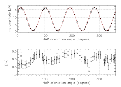
Figure 9: Data from a laboratory measurement of the modulation efficiency. The setup for this measurement is described in Section 6.2. The solid curve is the best fit model given by Equation 14. The reduced $\chi^{2}$ for this model is 1.03 for 42 degrees of freedom. From the fit parameters, we calculated $\mathcal{P}$ to be $0.88\pm 0.03$, which corresponds to polarimeter efficiency $\epsilon=0.94\pm 0.02$. The difference between these data and the best-fit model are plotted in the bottom panel to show the goodness-of-fit and the measurement error.

We define the modulation efficiency $\epsilon$ as the multiplicative factor that relates the measured data to the incident $Q$ and $U$ Stokes components, see Equation 3. It can be shown that for monochromatic light of frequency $\nu$

$$\epsilon_{\nu}=g\sin^{2}\frac{\delta(\nu)}{2},$$ (12)

where $\delta(\nu)$ is the retardance of the HWP and $g$ is the polarization efficiency of the wire-grid polarizer (Johnson, 2004; Collins, 2006). We calculated a typical expected efficiency

$$\epsilon_{exp}=\frac{\displaystyle\int\epsilon_{\nu}S(\nu)d\nu}{\displaystyle\int S(\nu)d\nu},$$ (13)

from the thickness of the HWP, the measured $g$, and a typical spectral response as a function of frequency $S(\nu)$. For MAXIPOL $g$ was measured to be $0.97$ (Johnson, 2004). The expected efficiency $\epsilon_{exp}$ was 93%, and this result agrees with the efficiencies measured in the laboratory and listed in Table 2 to within the 2% experimental uncertainty. The following section explains the laboratory measurement and analysis.

A wire-grid polarizer made from the same material used to make the polarization analyzer was mounted on the cryostat window with its transmission axis oriented to within $2^{\circ}$ of the axis of the analyzer. Beam filling thermal radiation from a 273 K ice bath was chopped at approximately 6.5 Hz with a 300 K aluminum chopper blade covered with absorbing foam (0.64 cm thick Eccosorb LS-14). In order to avoid bolometer saturation from the brightness of the warm loads, a 4 K absorptive attenuator (1.9 cm thick Eccosorb MF110) that was designed to transmit less than 3% at 140 GHz was inserted into the optical path at the intermediate focus of the telescope (Peterson & Richards, 1984; Johnson, 2004). The HWP was stepped in $\sim 5^{\circ}$ intervals and approximately 20 sec of data were collected at each HWP orientation. Detector drifts were removed by fitting a model consisting of a second-degree polynomial and a single-time-constant exponential to each data segment. The transmitted chop amplitude was estimated by subtracting the noise RMS, which was obtained from an independent noise-only measurement, from the data RMS. The effect of bolometer bath temperature drifts was mitigated by implementing a time-dependent responsivity correction. The detector response was linearized by applying a quadratic, amplitude dependent responsivity correction.

The data from one typical photometer are shown in Figure 9. The following five parameter model was fit to the binned data

$$m(\rho)=\!\!\!\! A_{2f_{o}} \!\!\!\!\cos(2\beta+\phi_{2f_{o}})$$

$$+\!\!\!\! A_{4f_{o}} \!\!\!\!\cos(4\beta+\phi_{4f_{o}})+B.$$ (14)

The nominal chop amplitude error per HWP orientation bin was estimated to be the detector noise RMS. This random error was assigned before responsivity corrections. The subsequent responsivity corrections caused the magnitude of the random error to vary from bin to bin. A systematic error was estimated by subtracting the best fit model from the binned data, computing the RMS of the residual and then adding this error in quadrature with the nominal error per bin. This combined error was used to compute the final errors in the fit parameters. The experimental figure of merit

$$\mathcal{P}=\frac{I_{max}-I_{min}}{I_{max}+I_{min}}$$ (15)

was calculated from the fit parameters using the equivalent expression $\mathcal{P}=A_{4f_{o}}/B$, and the error in $\mathcal{P}$ was propagated from the errors in $A_{4f_{o}}$ and $B$. Using Mueller calculus it can be shown that $\mathcal{P}$ and $\epsilon$ are related by

$$\epsilon=\frac{1+g^{2}}{g}\frac{\mathcal{P}}{1+\mathcal{P}},$$ (16)

and the value for $\epsilon$ for each photometer is given in Table 2. The agreement between $\epsilon$ and the expected modulation efficiency $\epsilon_{exp}$ (Equation 13) confirms that the 7% average depolarization for the 140 GHz photometers is accounted for by the efficiency of the grid polarizer and the spectral response of the HWP.

$\begin{array}[]{ccc}\includegraphics[width=216.81pt]{./f10a.eps}&&\includegraphics[width=216.81pt]{./f10b.eps}\\ \end{array}$

Figure 10: $Q$ and $U$ maps of the MAXIPOL observation region near $\beta$-UMi created from the raw data (left) and raw maps convolved with a 10 arcmin FWHM Gaussian beam (right). The pixel size is 3 arcmin. The convolved maps are used for visual inspection only.

7 Analysis and Results

We used a maximum-likelihood method to make maps of $Q$ and $U$ from the TOPD (see Figure 10). The map pixel size was set to 3 arcmin. Two approaches, one frequentist and one Bayesian, were used to estimate the $EE$, $BB$ and $EB$ angular power spectra in three $\ell$ bins: $\ell\leq 150$, $151\leq\ell\leq 693$ and $\ell\geq 694$. Given the beam size and the sky coverage we expect that only the center bin would have any signal. For both methods we used the $2.3^{\circ}\times 2.3^{\circ}$ region of the maps inside the white square in Figure 4. The average integration time in this box was 117 sec for each 3 arcmin pixel. A comprehensive description of the analysis is given in Wu et al. (2006). Here we only give a summary.

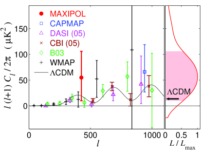
Figure 11: The MAXIPOL estimate of $EE$ power and other reported results (see Section 1 for references). The solid black line is the $\Lambda$CDM concordance model given by Spergel et al. (2006). The MAXIPOL result shown here is the 68% probability region around the maximum of the likelihood function without any priors on the EB or BB spectra. The likelihood function is shown in the right panel. The black arrow in this likelihood panel marks the expected $\Lambda$CDM signal for our bin, which is $14~{}\mu\mbox{K}^{2}$. Assuming a uniform prior the probability that the amplitude is positive is 96%. Including the calibration uncertainty does not change the significance of positive power and increases the error bars slightly, see text.

For the Bayesian analysis we estimated the amplitude of the angular power spectra using a Monte-Carlo Markov Chain algorithm (MacKay, 2003; Lewis & Bridle, 2002) derived from the MADCAP spectrum solver MADspec (Borrill et al., 2006). From a pair of 50,000 element chains we calculated the posterior likelihoods of the amplitudes of the power spectra in all 9 $\ell$ bins. Estimates for the amplitude were calculated both with and without priors which set the $EB$ and $BB$ spectra to zero with four different functions that describe the shape of the power spectrum within the bin. Here we quote the results for the amplitude of $\ell(\ell+1)C_{\ell}/2\pi$ after marginalization over the eight un-interesting $\ell$ bins and without any priors on the $EB$ and $BB$ power spectra. Results obtained with other assumptions are presented in Wu et al. (2006).

The left panel of Figure 11 shows the estimated maximum-likelihood $EE$ power and other reported results, while the right panel shows the corresponding posterior likelihood function. This result gives weak evidence for an $EE$ signal with a maximum-likelihood amplitude of $55_{-45}^{+51}~{}\mu\mbox{K}^{2}$ (68%). The likelihood function is asymmetric and skewed positive such that if we assume a uniform prior over all possible values of $\ell(\ell+1)C_{\ell}/2\pi$ (both positive and negative) the probability for a signal larger than zero is 96%. Including the calibration uncertainty the maximum-likelihood amplitude is $53_{-45}^{+57}~{}\mu\mbox{K}^{2}$ (68%) with no change in the probability of positive power. The $EE$ amplitude predicted by the concordance $\Lambda$CDM model given by Spergel et al. (2006) is $14~{}\mu\mbox{K}^{2}$. This theoretical value falls inside the 65% confidence region of our likelihood function around the maximum-likelihood value. The sharp cut-off on the negative end of the parameter axis is a consequence of correlations that occur within the high dimensionality of the marginalized space. Despite this feature, the likelihood accurately represents the result of the experiment (see Wu et al. (2006) for more details).

Both the 68% confidence intervals and the significance of positive power depend somewhat on the shape function used during the power spectrum estimation and on whether there are prior constraints on the $EB$ and $BB$ spectra. For example, assuming a uniform prior, the probability that the $EE$ power spectrum amplitude is positive is 83% for a shape function of $1/\ell(\ell+1)$ with $EB$ and $BB$ set to zero. The probability is 98% for a shape function of $1/(2\ell+1)$ with no constraints on $EE$ and $EB$.

The amplitudes of the $EB$ and $BB$ power spectra assuming the $1/\ell(\ell+1)$ shape function are $18_{-34}^{+27}$ and $-31_{-19}^{+31}~{}\mu\mbox{K}^{2}$ (68%), respectively, which are consistent with $\Lambda$CDM predictions. MAXIPOL does not have the sensitivity to detect either $BB$ or $EB$.

For the frequentist analysis we computed pseudo-band powers from the Fourier transform of the $Q$ and $U$ maps using the flat sky approximation. The pseudo-band powers have biases coming from the beam convolution, the time domain processing, and the Fourier transform. These biases were corrected, and band-power error bars were estimated using Monte Carlo simulations and the measured beam profiles. Results from the frequentist methods are consistent with those from the Bayesian analysis although the error computed by the Bayesian method is smaller, as expected.

8 Systematic Errors

8.1 Maps and Spectra

We tested the $Q$ and $U$ maps used in the power spectrum analysis for signal Gaussianity by analyzing the eigenvalue-normalized Karhunen-Loeve coefficients (Wu et al., 2001a). If the signal is Gaussian then these coefficients should be normally distributed. Some of the eigenvalues of the noise-whitened signal matrix were negative because of the high noise and imperfectly estimated signal in those modes. We excluded these modes from the test, but included noise-dominated modes. The resulting coefficients passed the Kolmogorov test for normality at 95% confidence.

To check for residual systematic errors we differenced maps from the first and second halves of the TOPD. The power spectra calculated from these difference maps give a result that is consistent with the absence of signal and with random noise. The maximum-likelihood value for the $EE$ power is $-19^{+54}_{-29}\mu$K² (68%).

8.2 Cross-Polarization

We refer to “cross-polarization” as a leakage between $Q$ and $U$ states of polarization as quantified by the $QU$ cross term of the appropriate Mueller matrix. Here, we describe characterization of the cross-polarization of the main beam.

Laboratory measurements outlined in Section 6.2 characterized effects due to the photometer dependent cross-polarization of the optical system, but without the effects of the primary mirror, combined with a photometer independent HWP encoder offset. Both effects were corrected in the analysis by using the photometer-dependent HWP angle $\beta$.

For the purpose of instrument characterization these two effects were separated by assuming that the center of the focal plane has zero cross-polarization because it is in the symmetry plane of the optical system. This assumption was supported by simulations of the optical system. The variation in the $\beta$ correction around this zero-point was interpreted as photometer dependent cross-polarization. The measurements show that the cross-polarization produces less than $3.4^{\circ}$ of linear polarization rotation for any photometer. This result agrees with ray-tracing simulations.

Simulations show that adding the primary mirror to the system should increase the linear polarization rotation induced by cross-polarization by less than $0.1^{\circ}$. This additional rotation was not corrected for during data analysis because calculations showed the level of error in the power spectrum produced by the effect was negligible.

Uncertainties in the angles $\alpha$ and $\beta$ (see Section 4) are predominantly small systematic offsets that are equivalent to unknown cross-polarization. The uncertainty in $\alpha$ is $2^{\circ}$ due to the uncertainty in the orientation of the balloon gondola during the pre-flight telescope alignment. The uncertainty in $\beta$ is less than $2^{\circ}$ due to the uncertainty in the alignment of the wire grid on the cryostat window during the polarization calibration, and due to the uncertainty in the knowledge of the bolometer time constants. According to simulation, these errors have a negligible impact on the results.

8.3 Instrumental Polarization

We refer to “instrumental polarization” as those effects that would produce a detection of polarized light even if an unpolarized light is incident on the instrument. With HWP polarimetry, polarized light that is produced on the sky side of the HWP is modulated and gives rise to a systematic signal at $4f_{0}$. The systematic signal can leak into the signal bandwidth, which is at a sideband of $4f_{0}$, if it varies with time.

In MAXIPOL several mechanisms contributed to an instrumental polarization signal at and near $4f_{0}$. Differential reflection of light by the primary, secondary and tertiary mirrors and by the polypropylene vacuum window of the cryostat produced partially polarized light in transmission. Of these, the reflection by the window was dominant. Emission from the mirrors and from the window produces partially polarized light because of the asymmetric nature of the optical system. Of these emission from the primary mirror was dominant. Unpolarized emission inside the cryostat that is diffracted around sharp edges into the light path can produce substantial polarization.

The instrumental polarization produced by these mechanisms was divided into two types: a stable polarized offset and a time varying instrumental signal that was synchronous with the sky. The stable offset appeared as the $4f_{o}$ component of the HWP synchronous signal that we discussed in Section 5.1. The photometer-dependent magnitude of this signal was in the range of 30 to 600 mK across the focal plane (see Section 5.1). Calculations show that instrumental polarization produced in transmission by differential reflection off the bowed polypropylene window of the cryostat will produce signals at the low end of this range. The upper end of this range is consistent with signals produced by diffraction from sharp edges of apertures within the cold optics box. This offset was stable on time scales much longer than data segments that were used for map making and therefore amplitude drifts did not leak into our signal band between 0.06 and 1.5 Hz (see Section 5.1 and Figure 6$(d)$). This stable signal was rejected both during subtraction of the HWP synchronous signal and during demodulation.

The time-varying instrumental signal was modulated with the intensity pattern on the sky, thereby leaking $I\rightarrow Q,U$ and therefore $T\rightarrow E,B$. It arose only through polarization produced in transmission. We measured this signal in two ways. The level of instrumental polarization produced by the receiver alone was determined to be less than approximately 1% for a typical 140 GHz photometer in the laboratory before flight. The procedure used for this measurement was essentially identical to the one outlined in Section 6.2. However, for this measurement the polarizer was removed from the cryostat window so the chopped signal observed an unpolarized load. During flight, the effect was measured more accurately with the full instrument during the Jupiter calibration scan. Since the level of polarization of Jupiter is expected to be small (Clemens et al., 1990) the planet served as an unpolarized point source. The instrumental polarization produced in transmission was measured by rotating the HWP during the beam-mapping procedure. The resulting $Q$ and $U$ beam maps of Jupiter yielded no detectable instrumental polarization signal above about 1% for ten of the twelve 140 GHz photometers. The remaining two photometers, which were located at the edge of the focal plane, detected instrumental polarization at the level of 4% and 5%. Calculations show that this level of instrumental polarization is plausible given a particular alignment between the focal plane and the window to the cryostat. Assuming conservatively that all photometers had approximately 4% instrumental polarization in transmission, simulations show that this performance would only produce a spurious 3 $\mu$K² signal in our $EE$ and $BB$ power spectra for the multipole bin of $\ell$ = 151 to 693. Since this leakage signal is undetectable in our data, no correction was applied during the analysis.

8.4 Foregrounds

The region of the sky near $\beta$-UMi was selected for CMB observations because contamination from dust, synchrotron and point sources is expected to be negligible. Polarized dust was our main concern because synchrotron radiation is brightest at frequencies below the MAXIPOL spectral bands, and point sources should not be polarized. Extrapolating from 100 $\mu$m using Finkbeiner model 8 (Finkbeiner et al., 1999), the unpolarized mean dust brightness over the $2.3^{\circ}\times 2.3^{\circ}$ square region used for power spectrum estimation should be 4.1 $\mu$K with an RMS of 0.8 $\mu$K. Archeops found a 5% polarized fraction for dust emission in the galactic plane (Benoit et al., 2004). The full sky WMAP 3-year data are consistent with this polarized fraction (Page et al., 2006). Given these measurements, the expected foreground polarization anisotropy over the $\beta$-UMi square region should be less than 0.04 $\mu$K RMS, which is not detectable by MAXIPOL. A catalog search yielded no detectable radio or infrared sources in our field (Sokasian et al., 2001). No foreground corrections were made during data analysis.

The data from the 420 GHz polarimeters can be used to improve the knowledge of the level of foreground dust contamination in the $\beta$-UMi region. However, this 420 GHz information was not used in this analysis for two primary reasons. First, the 420 GHz maps of Jupiter were poorly sampled so more work is required to determine the intensity calibration and the beam centers for pointing reconstruction. Second, the attenuator used for pre-flight polarimeter characterization (see Section 6.2) did not transmit detectable amounts of 420 GHz signal, so a dedicated 420 GHz post-flight polarimeter characterization is required to calibrate the TOPD of this data set.

9 Discussion

MAXIPOL was designed to be a pathfinder for bolometric CMB polarization experiments. It is the first bolometric CMB experiment to report results with a rapid polarization modulator.

The predicted benefits of the HWP technique have been demonstrated. Power spectra of the time domain data from the twelve independent polarimeters gave white noise after demodulation to frequencies well below 50 mHz for most of the data. A significant fraction of demodulated data had white noise at frequencies as low as 1 mHz. The $Q$ and $U$ data showed no detectable systematic errors despite a sizable HWP synchronous signal in the raw data. There was no need to compare noise and responsivity data between detectors, which is necessary when using differencing polarimeters. This made the analysis simpler.

We used the $Q$ and $U$ data to construct a map and estimate the polarization power spectra. The time domain noise was shown to be Gaussian and stationary. The noise in the map is consistent with Gaussian random noise at a level expected given instrument noise. The time streams and maps were subjected to multiple tests for systematic errors with null results.

The data give weak evidence for $EE$ power at a level that is consistent with the prevailing cosmological model. The $EB$ and $BB$ power spectra are consistent with zero, also as expected given instrument noise and the cosmological model.

MAXIPOL’s successful experience with a HWP will inform the design of future, more sensitive, experiments designed to characterize B-mode polarization of the CMB.

Appendix: Beam Mapping

The raw data collected during the Jupiter observations contained the following systematic errors: the HWP synchronous signal, low-frequency drifts, and transients. These spurious signals needed to be removed to make accurate beam maps. The magnitude of the Jupiter signal was similar to the magnitude of the HWP synchronous signal, so the algorithm described here was tailored for recovering signals that were much greater than the noise.

To remove the low-frequency drifts, we first removed a preliminary estimate of the HWP synchronous signal. This synchronous signal was modeled in this algorithm as,

$${\cal H}(t)=\sum_{n=1}^{8}\left(X_{n}+Y_{n}t\right)\,\cos\left(\,n\beta(t)+\Theta_{n}\,\right).$$ (17)

The fit parameters, $X_{n}$, $Y_{n}$, and $\Theta_{n}$ were estimated using the following two step procedure. First, to determine the phase of each Fourier component of the HWP synchronous signal, $\Theta_{n}$, the following cosine-wave model was fit to the raw data binned in the HWP angle domain:

$${\cal H}(\beta)=\sum_{n=1}^{8}Z_{n}\cos\left(\,n\beta+\Theta_{n}\,\right).$$ (18)

Here, $Z_{n}$ and $\Theta_{n}$ are the fit parameters, and $\Theta_{n}$ in Equation 17 is equal to $\Theta_{n}$ in Equation 18. The bin size was set to 1 deg. Given the HWP rotation frequency, this bin size prevented neighboring time samples from falling into the same bin. During the binning procedure, low-frequency noise was rejected in each bin by high-pass filtering the raw data in the frequency domain before binning; transients, and planet signals were rejected by setting the bin value equal to the mode, which was estimated by iteratively histogramming the bin data. In the second step of estimating the synchronous signal, the linearly varying amplitude of each Fourier component was found by fitting a line to the demodulated data in the time domain. For demodulation, the reference signal,

$${\cal R}(t)=\cos\left(\,n\beta(t)+\Theta_{n}\,\right),$$ (19)

was phase locked by construction because the best-fit phase, which was output from the previous step, was used for each Fourier component. An estimate of the HWP synchronous signal was then constructed using $\Theta_{n}$ from step one and $X_{n}$ and $Y_{n}$ from step two. This estimate was then subtracted from the raw data leaving only Jupiter signal, transients, low-frequency drifts, and noise.

Low-frequency drifts, which biased the beam maps if not subtracted, were removed from this data by iteratively fitting and subtracting second-degree polynomials from 24 sec long segments of data. This segment length was selected because it was much longer than a typical crossing time of Jupiter through the beam. After each iteration, the polynomial fit was subtracted and data points greater than 3 standard deviations away from zero were ignored in the subsequent fitting iterations. Given the 3 standard deviation rejection criteria, the polynomial estimates converged after three iterations. This masking procedure prevented transients and the planet signal from biasing the estimate of the low-frequency drifts.

The final drift estimate was subtracted from the raw data. The effects of the electronic filters and the bolometer time constants were deconvolved using the procedure given in Section 5.2. A second iteration of HWP synchronous signal estimation was required because the synchronous signal was phase shifted by the filter deconvolution. Transients larger than the empirically determined maximum Jupiter signal were flagged. The beams were then mapped using the telescope pointing, the transient flags, and the data with synchronous signal and low-frequency drifts subtracted. The map pixel size was set to 0.7 arcmin to allow accurate estimation of the $B_{\ell}$, which was used during CMB power spectrum estimation.

Biases in the beam map that were introduced by the low-frequency drifts were significant. To allowed for better estimation and subtraction of these drifts, the entire process outlined above was repeated with a Jupiter signal template removed during the low-frequency drift estimation. This signal template was computed by scanning a beam model with the telescope pointing. Here the beam model was the two-dimensional elliptical Gaussian that best fit the pixelized maps that were output from the first iteration of the process.

References

- Abroe et al. (2004) Abroe, M. E., et al. 2004, ApJ, 605, 607
- Balbi et al. (2000) Balbi, A., et al. 2000, ApJ, 545:L1; Erratum. 2001, ApJ, 558, L145
- Barkats et al. (2005) Barkats, D., et al. 2005, ApJ, 619, 2, L127
- Benoit et al. (2004) Benoit, A., et al. 2004, A & A, 424, 571
- Bock (1994) Bock, J. J. 1994, Ph.D. Thesis. University of California, Berkeley
- Borrill et al. (2006) Borrill, J., et al. 2006, in preparation
- Clemens et al. (1990) Clemens, D. P., et al. 1990, PASP, 102, 1064C
- Collins (2006) Collins, J. S. 2006, Ph.D. Thesis. University of California, Berkeley
- Finkbeiner et al. (1999) Finkbeiner, D. P., Davis, M. & Schlegel, D. J. 1999, ApJ, 524, 867
- Griffin et al. (1986) Griffin, M. J., et al. 1986, Icarus, 65, 244
- Hagman & Richards (1995) Hagmann, C. & Richards, P. L. 1995, Cryogenics, 35, 5, 303
- Hanany et al. (2000) Hanany, S., et al. 2000, ApJ, 545, L5
- Hinshaw et al. (2003) Hinshaw, G., et al. 2003, ApJS, 148, 63H
- Jaffe et al. (1999) Jaffe, A. H., et al. 1999, in Microwave Foregrounds, eds. A. de Oliveira-Costa & M. Tegmark (San Francisco: ASP)
- Johnson et al. (2003) Johnson, B. R., et al. 2003, New Astronomy Reviews, 47, 1067
- Johnson (2004) Johnson, B. R. 2004, Ph.D. Thesis, University of Minnesota
- Johnson et al. (2006) Johnson, B. R., et al. 2006, in Proceedings from the Rencontres de Moriond, in press
- Lee et al. (1998) Lee, A. T., et al. 1998, in EC-TMR Conference Proceedings 476, 3 K Cosmology, ed. L. Maiani, F. Melchiorri, & N. Vittorio (Woodbury, New York: AIP), 224, preprint (astro-ph/9903249)
- Lee et al. (2001) Lee, A. T., et al. 2001, ApJ, 561, L1
- Leitch et al. (2005) Leitch, E. M., et al. 2005, ApJ, 624, 10L
- Lewis & Bridle (2002) Lewis, A. & Bridle, S. 2002, Phys. Rev. D., 66, 10
- MacKay (2003) MacKay, D. J. C. 2003, Information Theory, Inference, and Learning Algorithms (Cambridge, UK: Cambridge University Press)
- Masi et al. (2006) Masi, S., et al. 2006, A&A, 458, 687
- Montroy et al. (2005) Montroy, T. E., et al. 2006, ApJ, 647, 813
- Page et al. (2006) Page, L., et al. 2006, ApJ, submitted, preprint (astro-ph/0603450)
- Peterson & Richards (1984) Peterson, J. B. & Richards, P. L. 1984, Int. J. Infrared Millimeterwaves, 5, 12, 1507
- Rabii (2002) Rabii, B. 2002, Ph.D. Thesis. University of California, Berkeley
- Rabii et al. (2006) Rabii, B. et al. 2006, Rev. Sci. Instrum., 77, 071101
- Readhead et al. (2004) Readhead, A. C. S., et al. 2004, Science, 306, 5697, 836
- Sokasian et al. (2001) Sokasian, A., Gawiser, E. & Smoot G. F. 2001, ApJ, 562, 88
- Spergel et al. (2006) Spergel, D.N., et al. 2006, ApJsubmitted, preprint (astro-ph/0603449)
- Stompor et al. (2001) Stompor, R., et al. 2001, ApJ, 561, L7
- Tinbergen (1996) Tinbergen, J. 1996, Astronomical Polarimetry (Cambridge, UK: Cambridge University Press)
- Winant (2003) Winant, C. D. 2003, Ph.D. Thesis. University of California, Berkeley
- Wu et al. (2001a) Wu, J.H.P., et al. 2001a, Phys. Rev. Lett., 87, 251303
- Wu et al. (2001b) Wu, J.H.P., et al. 2001b, ApJS, 132, 1
- Wu et al. (2006) Wu, J.H.P., et al. 2006, ApJ, in preparation (companion paper)
- Yoon et al. (2006) Yoon, K. W., et al. 2006. in Millimeter and Submillimeter Detectors and Instrumentation for Astronomy III, Proceedings of SPIE, 6275
- Zaldarriaga & Seljak (1997) Zaldarriaga, M. & Seljak, U. 1997, Phys. Rev. D., 55, 1830