Luminosity, selfgravitation and nonuniqueness of stationary accretion

Abstract

We investigate newtonian description of accreting compact bodies with hard surfaces, including luminosity and selfgravitation of polytropic perfect fluids. This nonlinear integro-differential problem reduces, under appropriate boundary conditions, to an algebraic relation between luminosity and the gas abundance in stationary spherically symmetric flows. There exist, for a given luminosity, asymptotic mass and the asymptotic temperature, two sub-critical solutions that bifurcate from a critical point. They differ by the fluid content and the mass of the compact centre.

I Introduction.

We study in this paper a newtonian accreting systems consisting of a compact body enclosed by a ball of selfgravitating gas. Our aim is to investigate the following inverse problem: assume that one knows the luminosity, total mass, asymptotic temperature (or, equivalently, the asymptotic speed of sound) and the equation of state of the gas. Assume that the gravitational potential has a fixed value at the boundary of a compact body, but the radius of the body is arbitrary to some extent. The question arises: can one specify the mass of the compact body? And if one can, is the specification unique? That issue is interesting in itself within the framework of astrophysics but it is also related to following fundamental physical aspect.

The standard point of view that compact objects of a mass exceeding several solar masses constitute black holes has been challenged by Mazur and Mottola Mazur , who developed the notion of gravatars — stars almost as compact as black holes but dispossessed of event horizons. Gravastars are supposed to be built from matter which violates energy conditions Hawking and therefore they can avoid the standard compactness limits (like the Buchdahl theorem Buchdahl ) or mass bounds. The concept of gravastars originated from the belief that the only place after Big Bang that quantum gravity could manifest is the collapse of matter to a pre-(event horizon) phase, and that quantum gravity effect may or can actually stop the collapse. Yet another conclusion, if one believes in this argument, is that the search for quantum gravity should start from the revision of the scenario of the gravitational collapse to a black hole.

The issue of the validity of gravastars to astrophysics can be verified, at least in principle, by observations. The fundamental question is whether observations can distinguish compact bodies endowed with a hard surface (gravastars) from black holes. Narayan Narayan presented observational arguments in favour of the existence of black holes. Abramowicz, Kluźniak and Lasota Abramowicz raised several objections, expressing their view that present accretion disk models are not capable to make distinction between accretion onto a black hole or a gravastar.

We choose below the simplest selfcontained model that can be interpreted as a radiating system. While we do not address directly the problem of distinguishing between a gravastar and a black hole, our results show that there is an ambiguity even in the newtonian level. There can exists at least two solutions (two compact stars with a hard surface) to the inverse problem described above. This is not quite unexpected. In a recent general-relativistic analysis (valid also in the newtonian limit) the mass accretion rate $\dot{M}$ behaves like $y^{2}(1-y)$, where $y=M_{\ast}/M$ is the ratio of (roughly) the mass of the compact core to the total mass Kinasiewicz . Thus there exists a maximum of $\dot{M}$ when $y=2/3$. The luminosity equals to the mass accretion rate $\dot{M}$ multiplied by the available energy per unit mass — the potential $\phi(R_{0})$ at the hard surface of a compact star. Hence this simple analysis of accretion would suggest the existence of two weakly luminous regimes: one rich in fluid with $m_{f}\approx M$ and the other with a small amount of fluid, $m_{f}/M\ll 1$. To a given luminosity $x$ might have corresponded two systems with different $y$’s. The actual situation in the case with the luminosity is less clear, because the luminosity impacts also the accretion rate $\dot{M}$ and there exists a complex algebraic relation $y=y(x)$, but the nouniqueness is still retained.

II The Shakura model.

Stationary accretion of spherically symmetric fluids with luminosities close to the Eddington limit has been investigated since the pioneering work of Shakura Shakura . In Shakura the gas pressure and its selfgravity have been ignored and the analysis has been purely newtonian. Later researchers included both these aspects later and extended the analysis onto relativistic systems (Thorne — Rezzola ). We will consider a spherically symmetric compact ball of a fluid falling onto a non-rotating compact body. The areal velocity $U$ of a comoving particle labelled by coordinates $(r,t)$ is given by $U(r,t)=\partial_{t}R$, where $t$ is a comoving (Lagrangian) time. $p$ denotes pressure, $L(R)$ and $L_{E}$ are the local and Eddington luminosities, respectively. The quasilocal mass $m(R)$ is defined by $\partial_{R}m(R)=4\pi R^{2}\varrho$. The mass accretion rate is

$$\dot{M}=-4\pi R^{2}\varrho U.$$ (1)

$\varrho$ is the baryonic mass density. The equation of state is taken to be polytropic, $p=K\varrho^{\Gamma}$ with $\Gamma$ being a constant, ($1<\Gamma\leq 5/3$). We assume a steady collapse of the fluid, which means that all its characteristics are constant at a fixed areal radius $R$: $\partial_{t}X|_{R=\mathrm{const}}=(\partial_{t}-(\partial_{t}R)\partial_{R})X=0$, where $X=\varrho,U,a^{2}$. $a=\sqrt{\partial_{\rho}p}$ is the speed of sound. Strictly saying, a stationary accretion must lead to the increase of the central mass. This in turn means that the notion of the ”steady accretion” is approximate — it demands that the mass accretion rate is small and the time scale is short, so that the quasilocal mass $m(R)$ does not change significantly. The total mass $m(R_{\infty})$ will be denoted by $M$. Furthermore, we assume that the radius $R_{\infty}$ of the ball of fluid and other boundary data are such that $U^{2}_{\infty}\ll\frac{m(R_{\infty})}{R_{\infty}}\ll a^{2}_{\infty}$.

The steadily accreting gas is described by a system of integro-(ordinary)-differential equations. They consist of the (Euler) momentum conservation equation

$$U\partial_{R}U=-{Gm(R)\over R^{2}}-{1\over\varrho}\partial_{R}p+\alpha{L(r)\over R^{2}},$$ (2)

the mass conservation

$$\partial_{R}\dot{M}=0$$ (3)

and the energy conservation

$$L_{0}-L(r)=\dot{M}\left({a^{2}_{\infty}\over\Gamma-1}-{a^{2}\over\Gamma-1}-{U^{2}\over 2}-\phi(R)\right).$$ (4)

The constant $\alpha$ is defined by $\alpha=\sigma/\left(4\pi m_{p}c\right)$, $L_{0}$ is the total luminosity and $\phi(R)$ is the newtonian gravitational potential. Strictly saying, in Eq. (4) should appear ${a^{2}_{\infty}\over\Gamma-1}+{U^{2}_{\infty}\over 2}-{M\over R_{\infty}}$ but this is well approximated by ${a^{2}_{\infty}\over\Gamma-1}$, due to the aforementioned boundary conditions.

We define the Eddington luminosity as that at the outermost layer of the accreting gas, that is as $L_{E}=GM/\alpha$, while the total luminosity $L_{0}$ is equal to the product of the mass accretion rate and the total available energy per unit mass $\phi_{0}\equiv|\phi(R_{0})|$, where $R_{0}$ is an areal radius of the boundary of the compact body, $L_{0}=\dot{M}\phi_{0}$ (Shakura ). The quantity $\phi_{0}$ is fixed and $R_{0}$ in the constructed configurations is by definition the areal radius at which the absolute value of the surface potential equals to $\phi_{0}$. Differentiating $\dot{M}$ with respect to $R$, using the equality $\partial_{R}a^{2}/(\Gamma-1)=a^{2}\partial_{R}\ln\varrho=\partial_{R}p/\varrho$ and combining the obtained equation with (2) yields the differential equation $\partial_{R}\ln L={\alpha\dot{M}\over R^{2}}.$ Its solution can be written in terms of the Eddington and total luminosities as follows

$$L=L_{0}\exp\left({-L_{0}\tilde{R}_{0}\over L_{E}R}\right).$$ (5)

Here $\tilde{R}_{0}\equiv GM/|\phi(R_{0})|$ is a kind of modified size measure of the compact body. In the case of test fluids $\tilde{R}_{0}=R_{0}$. In the case of gravastars one should assume that $|\phi(R_{0})|\sim c^{2}/2$ and $\tilde{R}_{0}\sim 2GM/c^{2}$ is the Schwarzschild radius; while gravastars would require the general-relativistic treatment, we believe that essential features will be the same as in the newtonian description.

III The mass accretion rate.

In what follows it is assumed that there exists a sonic point, but we believe that the same (nonuniqeness) result would have been obtained for subsonic solutions. The sonic horizon (sonic point) is a location where $|U|=a$. In the following we will denote by the asterisk all values referring to the sonic points, e.g. $a_{\ast}$, $U_{\ast}$, etc. Differentiation with respect the areal radius will be denoted as prime ^′. One finds from the mass conservation $U^{\prime}=-U\left(\left(\varrho^{\prime}/\varrho\right)+2/R\right)$. Inserting that into the Euler equation (2), one finds

$${\varrho^{\prime}\over\varrho}(a^{2}-U^{2})={2\over R}\left(U^{2}-{Gm\left(R\right)\over 2R}+{L\left(r\right)\alpha\over 2R}\right).$$ (6)

thus at the sonic point the three characteristics, $a_{\ast}$, $U_{\ast}$ and $M_{\ast}/R_{\ast}$ are related,

$$a_{\ast}^{2} = U_{\ast}^{2}={Gm\ast\over 2R_{\ast}}\left(1-{L_{\ast}\alpha\over GM_{\ast}}\right)=$$ (7)

$${Gm\ast\over 2R_{\ast}}\left(1-{L_{\ast}M\over L_{E}M_{\ast}}\right).$$

It is clear from (7) that in order to have a critical flow one should have

$${L_{\ast}M\over L_{E}M_{\ast}}<1.$$ (8)

It is useful to express the velocity $U$ and the mass density $\varrho$ in the following way

$$U=U_{\ast}\frac{R^{2}_{\ast}}{R^{2}}\left({a^{2}_{\ast}\over a^{2}}\right)^{1/(\Gamma-1)},$$ (9)

where $U_{\ast}$ is the negative square root, and

$$\varrho=\varrho_{\infty}\left(a/a_{\infty}\right)^{2/(\Gamma-1)},$$ (10)

where the constant $\varrho_{\infty}$ is equal to the mass density of collapsing fluid at the boundary $R_{\infty}$. There exist four stationary branches crossing at the sonic point, one of which is the accretion flow.

Define

$$x\equiv{L_{0}\over L_{E}},~{}~{}~{}~{}y\equiv{M_{\ast}\over M},~{}~{}~{}~{}\gamma\equiv{\tilde{R}_{0}\over R_{\ast}},$$

$$\Delta_{*}\equiv L_{0}-L_{\ast}-2\dot{M}a^{2}_{\ast}{L_{\ast}\over yL_{E}-L_{\ast}},$$

$$\Psi_{\ast}\equiv-\phi_{\ast}-{GM_{\ast}\over R_{\ast}}.$$ (11)

In new variables the necessary condition (8) for the existence of a sonic point reads $x\exp\left(-x\gamma\right)<y$. A straightforward algebra leads to the following equation

$$a^{2}_{\infty}-{5-3\Gamma\over 2}a^{2}_{\ast}=\left(\Gamma-1\right)\left({\Delta_{\ast}\over\dot{M}}-\Psi_{\ast}\right).$$ (12)

We shall assume that $\gamma<1$ and $x\gamma\ll 1$. From Eq. (7) follows now

$$U^{2}_{\ast}={GM_{\ast}\over 2R_{\ast}}\left(1-{x\over y}\exp\left(-x\gamma\right)\right).$$ (13)

Then $\Delta_{\ast}=0$ up to the first order while $\Psi_{\ast}=4G\pi\int_{R_{\ast}}drr\varrho$. One can show, using arguments similar to those applied later, that $|\Psi_{\ast}|\ll a^{2}_{\ast}$. Therefore (12) simplifies to

$${a^{2}_{\ast}\over a^{2}_{\infty}}={2\over 5-3\Gamma};$$ (14)

that is exactly the same result as in the Bondi model Bondi . A careful reader would notice that the above derivation requires that $\Gamma$ is somewhat smaller than 5/3.

The rate of the mass accretion $\dot{M}$ as given by (1) can be expressed in terms of the characteristics of the sonic point. One obtains, using equations (7) and (1), that

$$\dot{M}=G^{2}\pi^{2}M^{2}{\varrho_{\infty}\over a^{3}_{\infty}}\left(y-x\exp\left(-x\gamma\right)\right)^{2}\left(\frac{a_{\ast}^{2}}{a_{\infty}^{2}}\right)^{\frac{(5-3\Gamma)}{2(\Gamma-1)}}.$$ (15)

Now, one can can show in a way similar to that applied in the case of relativistic accretion (Kinasiewicz ) that under the previously assumed conditions and $R_{\ast}>>\tilde{R}_{0}$ one has $\varrho_{\infty}=\chi_{\infty}\left(M-M_{\ast}\right)=M\chi_{\infty}\left(1-y\right)$ for $\Gamma\in(1,5/3-\delta)$ with some small $\delta$.

More specifically, one needs to show that the energy conservation equation (4) yields

$${a^{2}(R)\over a^{2}_{\infty}}<1-\left(\Gamma-1\right){\phi(R)\over a^{2}_{\infty}};$$ (16)

bounding $|\phi(R)|$ from above by $GM/R$ one obtains

$${a^{2}(R)\over a^{2}_{\infty}}<1+\left(\Gamma-1\right){GM\over Ra^{2}_{\infty}}.$$ (17)

Therefore (10) implies $\varrho\leq\varrho_{\infty}\left(1+{GM\over Ra^{2}_{\infty}}\right)^{1/(\Gamma-1)}$. The conclusion follows now from using this bound in $M-M_{\ast}=\int_{V}dV\varrho$ and appealing to the asymptotic conditions laid down in the forthcoming text. The proportionality constant $\chi_{\infty}$ is roughly the inverse of the volume of the gas outside of the sonic sphere. Since the total luminosity $L_{0}=\phi(R_{0})\dot{M}$ and $a^{2}_{\ast}/a^{2}_{\infty}$ is given by (14), one obtains that

$$L_{0}=\phi_{0}G^{2}\pi^{2}{\chi_{\infty}M^{3}\over a^{3}_{\infty}}\left(1-y\right)\left(y-x\exp\left(-x\gamma\right)\right)^{2}\left({2\over 5-3\Gamma}\right)^{\frac{(5-3\Gamma)}{2(\Gamma-1)}}.$$ (18)

IV The analysis of the luminosity equation.

It is convenient to cast the formula (18) in terms of the relative luminosity, $x=L_{0}/L_{E}$,

$$x=\beta\left(1-y\right)\left(y-x\exp\left(-x\gamma\right)\right)^{2},$$ (19)

where $\beta=\chi_{\infty}\phi_{0}\alpha G\pi^{2}{M^{2}\over a^{3}_{\infty}}\left({2\over 5-3\Gamma}\right)^{\frac{(5-3\Gamma)}{2(\Gamma-1)}}$.

We shall analyze solutions of this cubic (with respect to the variable $y$) equation. One can show that there exist at least two solutions $y(x,\beta)$ for any parameter $\beta$, $0\leq\gamma<1$ and the relative luminosity $x$ smaller than a certain critical value $a$. We shall add the adjective ”critical” to all characteristics of this critical point; hence a critical luminosity is that corresponding to $x=a$. The obtained results are following.

Theorem. Define $F(x,y)\equiv x-\beta\left(1-y\right)\left(y-x\exp\left(-x\gamma\right)\right)^{2}$. Then

i) there exists a critical point $x=a,y=b$ of $F$, that is $F(a,b)=0$ and $\partial_{y}F(x,y)|_{a,b}=0$, with $a$ and $b$ satisfying $0<a<b<1$ and $b={2+a\exp\left(-a\gamma\right)\over 3},a=4\beta(1-b)^{3}$;

ii) For any $0<x<a$ there exist two solutions $y(x){{}^{+}_{-}}$ bifurcating from $(a,b)$. They are locally approximated by formulae

$$y{{}^{+}_{-}}=b\pm{\sqrt{(a-x)(b+a\exp(-a\gamma)(1-2a\gamma))}\over\sqrt{\beta(b-a\exp(-a\gamma))(1-a\exp(-a\gamma))}}.$$ (20)

iii) The relative luminosity $x$ is extremized at the critical point $(a,b)$.

Proof.

The two criticality conditions yield two equations

$$a-\beta(1-b)(b-a\exp(-a\gamma))^{2}=0,$$

$$b-a\exp(-a\gamma)=2(1-b).$$ (21)

From Eqs (21) one immediately obtains the desired expressions

$$b={2+a\exp\left(-a\gamma\right)\over 3},~{}~{}~{}~{}a=4\beta(1-b)^{3}.$$ (22)

Inserting the second of eqs (22) into the second equation in (21), one arrives at

$$b={2\over 3}+{4\beta\over 3}(1-b)^{3}\exp(-4\beta(1-b)^{3}\gamma).$$ (23)

Both sides of this equation are continuous functions of $b$ and at $b=0$ the right hand side of (23) is bigger than the left hand side, while at $b=1$ the opposite holds true. Therefore there exists a solution. A closer inspection shows that there is only one critical solution. This fact actually guarantees that solutions $y(x)$ that bifurcate from $(a,b)$ extend onto the whole interval $x\in(0,a)$. (Hint: use the implicit function theorem and the fact that $(a,b)$ is the unique critical point). The specific form of a solution close to a critical point can be obtained as follows. Insert $x=a+\epsilon,y=b+y(\epsilon)$ into $F(x,y)=0$ and expand $F$ keeping the terms of lowest order. One obtains a reduced algebraic equation

$$\left(1+2\beta\left(1-b\right)\left(b-ae^{-a\gamma}\right)\left(ae^{-a\gamma}\gamma-e^{-a\gamma}\right)\right)\epsilon+$$

$$\beta\left(3b-1-2ae^{-a\gamma}\right)y^{2}(\epsilon)=0.$$ (24)

Notice that at the critical point $3b-1-2a\exp(-a\gamma)=1-a\exp(-a\gamma)$ (see the second of Eqs (21) ) while

$$2\beta\left(1-b\right)\left(b-a\exp(-a\gamma)\right)\left(a\exp(-a\gamma)\gamma-\exp(-a\gamma)\right)=$$

$$2a\left(a\exp(-a\gamma)\gamma-\exp(-a\gamma)\right)/(b-a\exp(-a\gamma).$$ (25)

Inserting (25) into (24) and finding $y(\epsilon)$ from the latter immediately leads to the approximate solution of ii).

Now we shall prove the third part of the Theorem. Let $(x_{0},y_{0})$ be a non-critical solution of $F(x,y)=0$ with the domain being subset $xe^{-x}<y$ of the square $0<x<1,0<y<1$. Then from the implicit function theorem there exists a curve $x(y)$ such that $F(x(y),y)=0$ for $y$ belonging to some vicinity of $y_{0}$. Along this curve one has

$${dx\over dy}=\beta{\left(y-xe^{-x\gamma}\right)\left(3y-2-xe^{-x\gamma}\right)\over 1+2\beta(1-y)(y-xe^{-x\gamma})(e^{-x\gamma}-\gamma xe^{-x\gamma})}.$$ (26)

The denominator is strictly positive while the nominator vanishes only at critical points. That proves the assertion. It follows from the form of the approximated solution constructed in part ii) that $x=a$ is the extremal value of the relative luminosity. That ends the proof of the Theorem.

It is easy to observe that the coordinates $a,b$ of the critical point increase with the increase of the parameter $\beta$. Indeed, from Eq. (22) follows ${da\over db}=e^{-a\gamma}(1-a\gamma)$; this is bigger than zero, since $a\gamma<1$. Differentiation of the first equation in (22) with respect to $\beta$ yields ${db\over d\beta}=4(1-b)^{3}/({da\over db}+12\beta(1-b)^{2})>0$; we exploited here the fact that ${da\over db}>0$. Since along the critical curve ${da\over d\beta}={da\over db}{db\over d\beta}$, we obtain also ${da\over d\beta}>0$. In the particular case of $\gamma=0$ one can explicitly find $b$ by solving (23),

$$b=1-{\left(\beta^{2}+\beta^{3/2}\sqrt{1+\beta}\right)^{2/3}-\beta\over 2\beta\left(\beta^{2}+\beta^{3/2}\sqrt{1+\beta}\right)^{1/3}};$$ (27)

(22) gives then $a(\beta)$ and one can check explicitly that both $a$ and $b$ monotonically increase with the increase of $\beta$. The forthcoming figure shows the two branches $x_{1}(y),x_{2}(y)$ bifurcating from a critical point, in the case when $\gamma=0$.

The next interesting fact is that at critical points the parameter $b$ is not smaller than 2/3. This lower bound is saturated at small $\beta$, i. e., when the relative luminosity $a$ is small (notice that $a<\beta$), which corresponds to the maximal rate of the mass accretion in irradiating systems Kinasiewicz . Since the fluid abundance is equal to $1-b$, we can conclude that critical configurations have less fluid than 1/3 of the total mass, and the upper bound 1/3 is saturated in the limit of vanishing radiation. The maximal mass accretion rate does not occur exactly at $y=2/3$, as in systems with no radiation Kinasiewicz , but at a somewhat larger value.

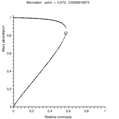
Figure 1: Here $\beta=50$. The mass abundance is put on the ordinate while the relative luminosity $x$ is shown on the abscissa. The circle encloses the bifurcation point $(a,b)$.

V Discussion.

In the foregoing text we have assumed the existence of an accreting system satisfying particular boundary conditions. Although the detailed behaviour is given by the integro-differential nonlinear system (2-4), its essential features can be deduced from the algebraic equation (19). The validity of this projection of the original equations to the algebraic problem relies on the existence of appropriate solutions. We checked numerically that there do exist such solutions and that the relative error made in the above approximations is of the order of $10^{-3}$. Here follows an example.

The mass of the system is 100 solar masses ($M=1.989\times 10^{35}$ grams), its size $1.254\times 10^{14}$ cm and the relative luminosity $x\equiv{L_{0}\over L_{E}}=0.1$. The adiabatic index was taken $\Gamma=4/3$, the asymptotic speed of sound $a^{2}_{\infty}=1.875\times 10^{7}$ cm/s and $\tilde{R}_{0}=6\times 10^{7}$ cm. Let us remark that if $M$ and $\tilde{R}_{0}$ are fixed, then also the potential at the surface of the compact core is fixed. The set of quantities hitherto specified should in principle determine a solution; any additional information would lead to a contradiction.

We have found, by integrating the original integro-differential equations (2 — 4) that there exist two solutions with following characteristics: i) solution I — $R_{\ast}=1.2\times 10^{5}$ cm, $M_{\ast}=0.11M$ and $\varrho_{\infty}\approx 2.144\times 10^{-8}$ g/cm³; ii) solution II — $R_{\ast}=1.068\times 10^{7}$ cm, $M_{\ast}=0.9999M$ and $\varrho_{\infty}\approx 2.41\times 10^{-12}$ g/cm³. The only difference between numerical solutions and algebraic approximations shows in $\varrho_{\infty}$ and it is of the order of 0.1% .

Under a simplifying assumption that $\gamma\ll 1$ one can neglect the exponential term in $x\exp(-x\gamma)$. The analysis of (22) and (27) allows us to conclude that $a$ can be as close as one wishes to 1 for large $\beta$. Putting that in physical terms, the luminosity $L_{0}$ can be close to the Eddington luminosity $L_{E}$ if the parametr $\beta$ is large enough, or more precisely, if the product $(M/M_{0})^{2}/(a_{\infty}/a_{0\infty})^{3}$ (where $M_{0}$ and $a_{0\infty}$ are some reference quantities) is large enough. The two bifurcation solutions have a luminosity $x<a$ and they are characterized by two different numbers $y_{1},y_{2}$; the latter can be markedly different (say $y_{1}>10y_{2}$) only for $x\ll a$. This is suggested by the point ii) of the Theorem which shows the branching of the two solutions from a critical point, but numerical calculations confirm that more precisely. A practical conclusion is a follows: if a given system radiates with the luminosity close to its critical luminosity (and, in particular, to the Eddington limit), then the cores corresponding to the bifurcating solutions have similar masses. The necessary and sufficient conditions for having two cores with significantly differing masses, $M_{1}\ll M_{2}$, is that the luminosity is much smaller than $L_{E}$ or the critical luminosity $a$, respectively.

VI Final remarks.

In conclusion, we have proven that there exist two radiating systems having the same mass, luminosity, asymptotic temperature and surface potential. In extreme cases — for instance when the total mass is very large and the luminosity low — one of the solutions corresponds to a compact body having a mass close to the total mass and a small amount of gas, while the other solution consists of a light compact body enclosed by a heavy cloud of gas. Returning to the question touched at the beginning - one would not make a distinction between a gravastar and a neutron star within the simple model discussed here.

There is a number of obvious questions that can be asked in connection with presented results.

The first question is whether one can justify the assumption — which we make — of stationary accretion in the case of a system where the cloud of accreting gas is heavier than the compact core. The resolution of this problem would require the investigation of the dynamical version of the Shakura model. The stationary solution of equations (2 — 4) should be inserted as initial data to the dynamical equations and if the dynamical solutions remains close to the stationary data then the assumption would be said to be justified. We performed an analogous verification of the assumption of stationarity in the case of selfgravitating gas (in the framework of general relativity) (Kinasiewicz , Mach ) with the positive conclusion. The evolving system remained essential unchanged in its interior for times much smaller than ($R_{\infty}/a_{\infty}$). We believe that the same conclusion will be valid for the Shakura model.

The second question is — accepting that the approximation of steady accretion is correct — whether one can reduce the integro-differential problem to an algebraic one. Our paper provides a proof that this is so if a solution satisfies particular boundary data. Numerical examples suggest that the set of solutions that satisfy the required boundary conditions is not empty. On the other hand, we believe that this nonuniqueness of solutions will manifest in a much larger set of steadily accreting systems which do not necessarily satisfy our boundary conditions; that it can be generic. The restriction to a particular sample of systems was made only in order to simplify the analysis.

Finally, there arises the question that inspired the paper: whether one can unambiguously distinguish between accretion onto compact bodies from accretion onto a black hole. This would require the extension of the above into general-relativistic systems. That is, from the general-relativistic point view, a straightforward exercise (see for instance malec ). There is, however, a fundamental difficulty (Thorne — Rezzola ) in describing interaction between accreting perfect fluid and the nonisotropic (and thus nonperfect) outflowing radiation. This introduces another level of ambiguity into the problem, but we believe that the nonuniqueness, that was discovered in the newtonian accretion will remain.

This paper has been partially supported by the MNII grant 1PO3B 01229.

References

- (1) P. O. Mazur and E. Mottola (Los Alamos), Proc. Nat. Acad. Sci. 101, 9545(2004).
- (2) S. W. Hawking and G. F. R. Ellis, The Large Scale Structure of Space-Time, Cambridge University Press (1975).
- (3) A. H. Buchdahl, Phys. Rev 116, 1027(1957).
- (4) A. E. Broderick and R. Narayan, ApJ. 638, L21(2006).
- (5) M. Abramowicz, W. Kluźniak and J.-P. Lasota, Astron. and Astrophys., 396, L31(2002).
- (6) J. Karkowski, B. Kinasiewicz, P. Mach, E. Malec and Z. Świerczyński, Phys. Rev. D73, 021503(R)(2006).
- (7) B. Kinasiewicz, P. Mach and E. Malec, Selfgravitation in a general-relativistic accretion of steady fluids, gr-qc/0606004.
- (8) N. I. Shakura, Astr. Zh 18, 441(1974).
- (9) T. Okuda and S. Sakashita, Astrophys. Space Sci., 52, 350(1977).
- (10) K. S. Thorne, R. A. Flammang and A. N. Żytkow, Mon. Not. R. Astron. Soc., 194, 475(1981).
- (11) M. G. Park and G. S. Miller, ApJ, 371, 708(1991).
- (12) L. Rezzolla and J. C. Miller, Class. and Quant. Grav.,11, 1815(1994).
- (13) H. Bondi, Mon. Not. R. Astron. Soc. 112, 192(1952).
- (14) E. Malec, Phys. Rev. D60, 104043 (1999).