The asymmetric relations among galaxy color, structure, and environment

Abstract

We investigate the dependences of galaxy star-formation history and galaxy morphology on environment, using color and $\mathrm{H}\alpha$ equivalent width as star-formation history indicators, using concentration and central surface brightness as morphological indicators, and using clustocentric distance as an environment indicator. Clustocentric distance has the virtue that it can be measured with very high precision over a large dynamic range. We find the following asymmetry between morphological and star-formation history parameters: star-formation history parameters relate directly to the clustocentric distance while morphological parameters relate to the clustocentric distance only indirectly through their relationships with star-formation history.This asymmetry has important implications for the role that environment plays in shaping galaxy properties and it places strong constraints on theoretical models of galaxy formation. Current semi-analytic models do not reproduce this effect.

1 Introduction

It has been known for quite some time that the statistical properties of galaxies are closely related to their surrounding environments. Much of previous environment-related work focused on the relationship between morphology and environment (e.g., Hubble 1936; Oemler 1974; Dressler 1980; Postman & Geller 1984; or the more recent work of Hermit et al. 1996; Guzzo et al. 1997; Giuricin et al. 2001; Trujillo et al. 2002). All these works find that bulge-dominated galaxies are more strongly clustered than disk-dominated galaxies. Since spectroscopic and photometric properties of galaxies are strongly correlated with morphology, it is not surprising to find that the spectroscopic and photometric properties of galaxies are also functions of environment (e.g., Kennicutt 1983; Hashimoto et al. 1998; Balogh et al. 2001; Martínez et al. 2002; Lewis et al. 2002; Norberg et al. 2002; Hogg et al. 2003, 2004; Kauffmann et al. 2004; Zehavi et al. 2005).

Since regions of the Universe with different densities evolve at different rates, we expect these environment dependencies to contain crucial information about galaxy formation and evolution. Considering that all of the observed statistical properties of galaxies appear to be interdependent, it is important to ask which properties are correlated with environment independently of the others; i.e., which environment relationships are fundamental and which ones are merely the products of other relations.

Blanton et al. (2005a) found that, out of color, luminosity, surface brightness, and radial concentration, the color and luminosity of a galaxy appear to be the only properties that are directly related to the local overdensity. Surface brightness and concentration appear to be related to the environment only through their relationships with color and luminosity. The main limitations in this study were caused by their environment indicator, local overdensity, since it has relatively low signal-to-noise and it cannot resolve scales smaller than $\sim 1$ Mpc. In a similar study, Christlein & Zabludoff (2005) used the clustocentric distance as an environment indicator found that there is a residual dependence of ongoing star formation on environment among galaxies of similar morphology, stellar mass, and mean stellar age. This study was limited by a relatively small sample size (1,637 galaxies in 6 clusters) as well as by the star formation indicator, OII, which is sensitive to dust and metallicity.

In this short paper, we build upon previous studies in several ways. We conduct a study similar to Blanton et al. (2005a), except that we use the clustocentric distance as our environment indicator. The clustocentric distance—the distance to the nearest galaxy cluster center—is a fundamental and precisely measurable environment indicator; indeed it can be measured at much higher signal-to-noise than estimates of overdensity on fixed scales. Thus, we probe the findings of Blanton et al. (2005a) on much smaller scales and at much higher signal-to-noise. We use the Berlind et al. (2006) cluster catalog that was created with an algorithm that made no use of galaxy colors, so our galaxy colors are unbiased even in the cluster cores. The cluster catalog was designed to recover groups of galaxies that are bound in the same underlying dark matter halo. In order to determine whether our results can be easily understood within our current understanding of galaxy formation and evolution, we compare our observational results from the Sloan Digital Sky Survey to analogous results from the semi-analytic Millennium simulation of galaxy formation (Croton et al., 2006).

In what follows, a cosmological world model with $(\Omega_{\mathrm{M}},\Omega_{\mathrm{\Lambda}})=(0.3,0.7)$ is adopted, the Hubble constant is parameterized as $H_{0}\equiv 100\,h~{}\mathrm{km\,s^{-1}\,Mpc^{-1}}$, and for the purposes of calculating distances and volumes $h=1$ except where otherwise noted (e.g., Hogg, 1999).

2 Data and Analysis

2.1 Observations

The SDSS has taken $ugriz$ CCD imaging and spectroscopy of many $10^{5}$ galaxies at $r<17.77~{}\mathrm{mag}$ (e.g., Gunn et al., 1998; York et al., 2000; Stoughton et al., 2002). All the data processing, including astrometry (Pier et al., 2003), source identification, deblending and photometry (Lupton et al., 2001), calibration (Fukugita et al., 1996; Smith et al., 2002), spectroscopic target selection (Eisenstein et al., 2001; Strauss et al., 2002; Richards et al., 2002), spectroscopic fiber placement (Blanton et al., 2003a), spectral data reduction and analysis (Schlegel & Burles, in preparation, Schlegel in preparation) are performed with automated SDSS software.

Galaxy colors are computed in fixed bandpasses, using Galactic extinction corrections (Schlegel et al., 1998) and $K$ corrections (computed with kcorrect v3_2; Blanton et al., 2003). They are $K$ corrected to the redshift $z=0$ observed bandpasses so they can be directly compared to the rest-frame SDSS $ugriz$ outputs of the Millennium simulation (Croton et al., 2006).

For the purposes of computing large-scale structure statistics, we have assembled a complete subsample of SDSS galaxies known as the NYU LSS sample14. This subsample is described elsewhere (Blanton et al., 2005b); it is selected to have a well-defined window function and magnitude limit. In addition, the galaxies in the sample used here were selected to have apparent magnitudes in the range $14.5<r<17.77~{}\mathrm{mag}$, redshift in the range $0.015<z<0.068$, and absolute magnitude $M_{{}^{0.1}i}>-24~{}\mathrm{mag}$. These cuts left 52,485 galaxies.

A seeing-convolved Sérsic model is fit to the azimuthally averaged radial profile of every galaxy in the observed-frame $i$ band, as described elsewhere (Blanton et al., 2003b; Strateva et al., 2001). The Sérsic model has surface brightness $I$ related to angular radius $r$ by $I\propto\exp[-(r/r_{0})^{(1/n)}]$, so the parameter $n$ (Sérsic index) is a measure of radial concentration (seeing-corrected). At $n=1$ the profile is exponential, and at $n=4$ the profile is de Vaucouleurs. In the fits shown here, values in the range $0.5<n<5.5$ were allowed.

To every best-fit Sérsic profile, the Petrosian (1976) photometry technique is applied, with the same parameters as used in the SDSS survey. This supplies seeing-corrected Petrosian magnitudes and radii. A $K$-corrected surface-brightness $\mu_{{}^{0.0}i}$ in the ${}^{0.0}i$ band is computed by dividing half the $K$-corrected Petrosian light by the area of the Petrosian half-light circle.

The $\mathrm{H}\alpha$ line flux is measured in a 20 Å width interval centered on the line. Before the flux is computed, a best-fit model consisting of scaled old-galaxy and A-star spectra (Quintero et al., 2004) is scaled to have the same flux continuum as the data in the vicinity of the emission line and subtracted to leave a continuum-subtracted line spectrum. This method fairly accurately models the $\mathrm{H}\alpha$ absorption trough in the continuum, although in detail it leaves small negative residuals. The flux is converted to a rest-frame EW with a continuum found by taking the inverse-variance-weighted average of two sections of the spectrum about 150 Å in size and on either side of the emission line. Further details are presented elsewhere (Quintero et al., 2004).

A caveat to this analysis is that the 3 arcsec diameter spectroscopic fibers of the SDSS spectrographs do not obtain all of each galaxy’s light because at redshifts of $0.015<z<0.068$ they represent apertures of between $0.6$ and $2.7~{}h^{-1}\,\mathrm{kpc}$ diameter. Consequently the integrity of our $\mathrm{H}\alpha$ EW measurement is a function of galaxy size, inclination, and morphology. We have looked at variations in our $\mathrm{H}\alpha$ EW results as a function of redshift and found that the quantitative results differ but our qualitative results remain the same.

We use the group and cluster catalog described in Berlind et al. (2006). The catalog is obtained from a volume-limited sample of galaxies that is complete down to an ${}^{0.1}r$ band absolute magnitude of $M_{r}<-19$ mag and goes out to a redshift of 0.068. Groups are identified using a friends-of-friends algorithm (see e.g., Geller & Huchra 1983; Davis et al 1985) with perpendicular and line-of-sight linking lengths equal to 0.14 and 0.75 times the mean inter-galaxy separation, respectively. These parameters were chosen with the help of mock galaxy catalogs to produce galaxy groups that most closely resemble galaxy systems that occupy the same dark matter halos. The resulting catalog contains 985 systems of richness $N_{\mathrm{gal}}\geq 5$ galaxies with an r-band absolute magnitude limit of $M_{r}<-19$ mag. For consistency, we call these objects “clusters”. Note that, unlike some other catalogs, galaxy colors are not used in cluster identification.

Berlind et al. (2006b, in preparation) calculate rough mass estimates for the clusters using the cluster luminosity function (where luminosity is defined as the total luminosity in $M_{r}<-19$ mag galaxies in the cluster) and assuming a monotonic relation between a cluster’s luminosity and the mass of its underlying dark matter halo. By matching the measured space density of clusters to the theoretical space density of dark matter halos (given the concordance cosmological model and a standard halo mass function), they assign a virial halo mass to each cluster luminosity. The masses derived in this way ignore the scatter in mass at fixed cluster luminosity and are only meant to be approximate. The median mass estimate for the clusters used here is $3\times 10^{13}$ solar masses. Each cluster has an associated “virial radius” of

$$R_{\mathrm{vir}}=\left(\frac{3}{4\,\pi}\frac{M}{200\,\rho_{o}}\right)^{\frac{1}{3}}\quad,$$ (1)

where $M$ is the estimated mass of the cluster and $\rho_{o}$ is the current mean density of the Universe. By this method, the median estimated virial radius for the clusters used here is $\sim 1$ Mpc. Note that this method for determination of the virial radii is very different from that employed by other investigators. Some have used a quasi-empirical formula based on velocity dispersion (Gomez et al., 2003; Christlein & Zabludoff, 2005), others have assumed that cluster mass is directly proportional to richness (Lewis et al., 2002); in general these methods differ substantially, and produce cluster catalogs with very different mass functions.

We use the cluster centers given by Berlind et al. (2006), which are computed as the mean of the member galaxy positions. We then calculate the transverse projected clustocentric distance $D_{\mathrm{cl}}$ from each galaxy to its nearest cluster center on the sky within $\pm 1000~{}\mathrm{km\,s^{-1}}$ in radial velocity.

2.2 Simulations

To better understand our observations, we do a similar analysis for the Millennium simulation galaxy catalog. The Millennium simulation is a large cosmological N-body simulation of $2160^{3}$ dark matter particles in a $500^{3}~{}\,h^{-3}\mathrm{Mpc^{3}}$ box. The formation of galaxies is simulated by using a semi-analytical model whose parameters and assumptions are tweaked in order to reproduce the joint luminosity-color, morphology, gas mass, and central black hole mass distributions of low-redshift galaxies. For a more detailed description, see Croton et al. (2006).

The publicly available output of this simulation (Croton et al., 2006) is a catalog of $\sim 9$ million galaxies that contains positions, velocities, bulge and total SDSS-band magnitudes, bulge and total masses, gas masses (cold, hot, and ejected), black hole masses, and star formation rates.

From this catalog we use the ratio of bulge-to-total luminosity as a morphology indicator. This $B/T$ value is an analog to our observed concentration and surface brightness. Similarly, we use the star formation rate SFR and SDSS-band ${}^{0.0}[g-r]$ color from this catalog as star-formation history indicators; these are analogs to our $\mathrm{H}\alpha$ EW and ${}^{0.0}[g-r]$ color measurements, respectively.

Before running the cluster-finding algorithm (Berlind et al., 2006), we distort the Millennium coordinates to mimic redshift-space distortions by changing the output coordinates of each galaxy from $[(x),(y),(z)]$ to $[(x),(y),(z+\frac{v_{z}}{H_{0}})]$. We then run the same friends-of-friends algorithm that we did on the data, using the perpendicular linking length in the $x-$ and $y-$directions and the line-of-sight linking length in the $z$-direction. After creating this cluster catalog we calculate each galaxy’s clustocentric distance using a similar algorithm we use on the data: We calculate the transverse projected clustocentric distance $D_{\mathrm{cl}}$ from each galaxy to its nearest cluster center on the $x-y$ plane within $\pm 10\,\mathrm{Mpc}$ in the $z$-direction.

3 Results

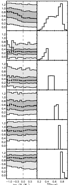
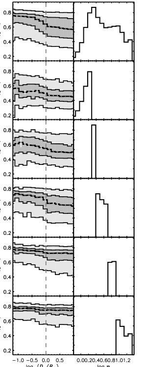
Figure 1: The dependence of radial concentration $n$ (left grid) and ${}^{0.0}[g-r]$ color (right grid) on clustocentric distance $D_{\mathrm{cl}}$. For the $2\times 6$ grid on the left, the top-left panel shows how the 5, 25, 50 (in bold), 75, and 95 percentiles of the distribution of concentration $n$ (Sérsic index) depend on clustocentric distance $D_{\mathrm{cl}}$ for the entire sample. The top-right panel of this grid shows the ${}^{0.0}[g-r]$ color distribution of the entire sample. The errors in the 50 percentile, calculated using the jackknife method (10 jackknife trials in each of which a contiguous 1/10 of the survey footprint is dropped) are overplotted in white (they are tiny). The subsequent rows show the same but for narrow color subsamples (color quintiles). The $2\times 6$ grid on the right is very similar but with the $n$ and ${}^{0.0}[g-r]$ properties interchanged. The left $2\times 6$ grid shows that in color subsamples, there is no residual dependence of concentration on environment, while the right $2\times 6$ grid shows that in concentration subsamples, there is a residual dependence of color on environment. This asymmetry is the principal result of this paper.

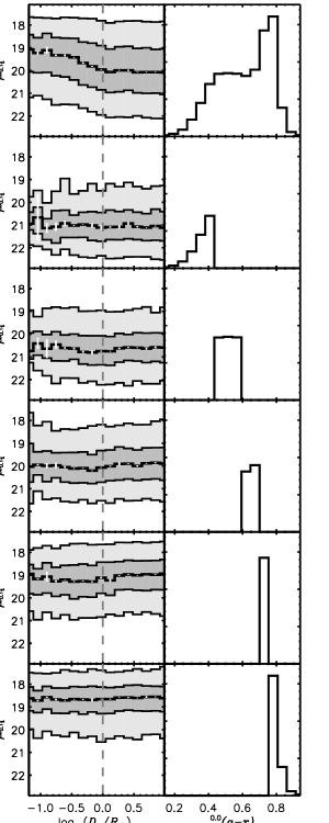
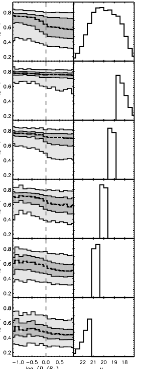
Figure 2: Similar to Figure 1, except replacing the radial concentration $n$ with surface brightness $\mu_{{}^{0.0}i}$. Notice the asymmetry seen in Figure 1 also occurs here.

Figure 1 shows how radial concentration and color relate to clustocentric distance within narrow subsamples of each other. For the $2\times 6$ grid on the left, the top-left panel shows how the 5, 25, 50 (in bold), 75, and 95 percentiles of the concentration distribution vary with clustocentric distance for the entire sample. The color distribution for the entire sample is shown in the right panel. The gradient in the concentration percentiles show that galaxies with small clustocentric distances tend to be more concentrated. The subsequent rows show the same relation but for narrow color subsamples whose color distribution is shown in the right panels. Notice the gradient seen in the top panel nearly vanishes for the narrow color subsamples below. The absence of a concentration gradient for these subsamples shows that at fixed color, there is no dependence of concentration on environment. The right $2\times 6$ grid shows the same plot but with concentration and color interchanged. Notice that a color gradient remains when looking at narrow concentration subsamples. This shows that at fixed concentration, there is a residual dependence of color on environment. The asymmetry seen in this figure is also seen in Figure 2 which uses surface brightness, instead of concentration, as a morphology tracer. This asymmetry is the principal result of this paper. This asymmetry is similar to that found by Blanton et al. (2005a), but it appears here at much higher significance and over a larger dynamic range.

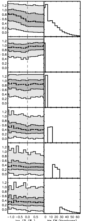
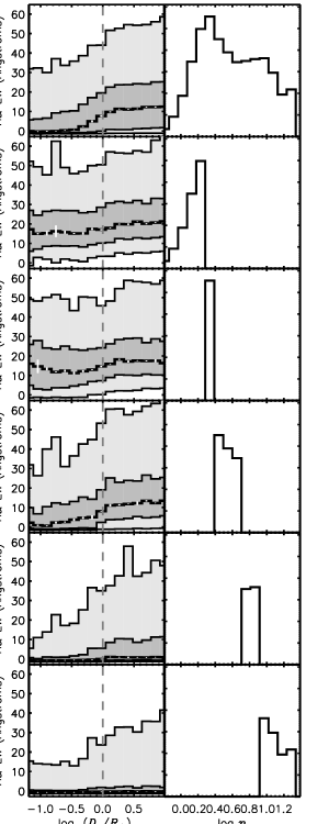
Figure 3: Similar to Figure 1, except replacing the ${}^{0.0}[g-r]$ color with our other star-formation history indicator: $\mathrm{H}\alpha$ emission line equivalent width ($\mathrm{H}\alpha$ EW). Notice the asymmetry seen in Figure 1 also occurs here.

Figure 3 also shows the same asymmetry shown in Figure 1 but using $\mathrm{H}\alpha$ EW, instead of color, as our star-formation-history parameter. Note that the right $2\times 6$ grid agrees with the findings of Christlein & Zabludoff (2005).

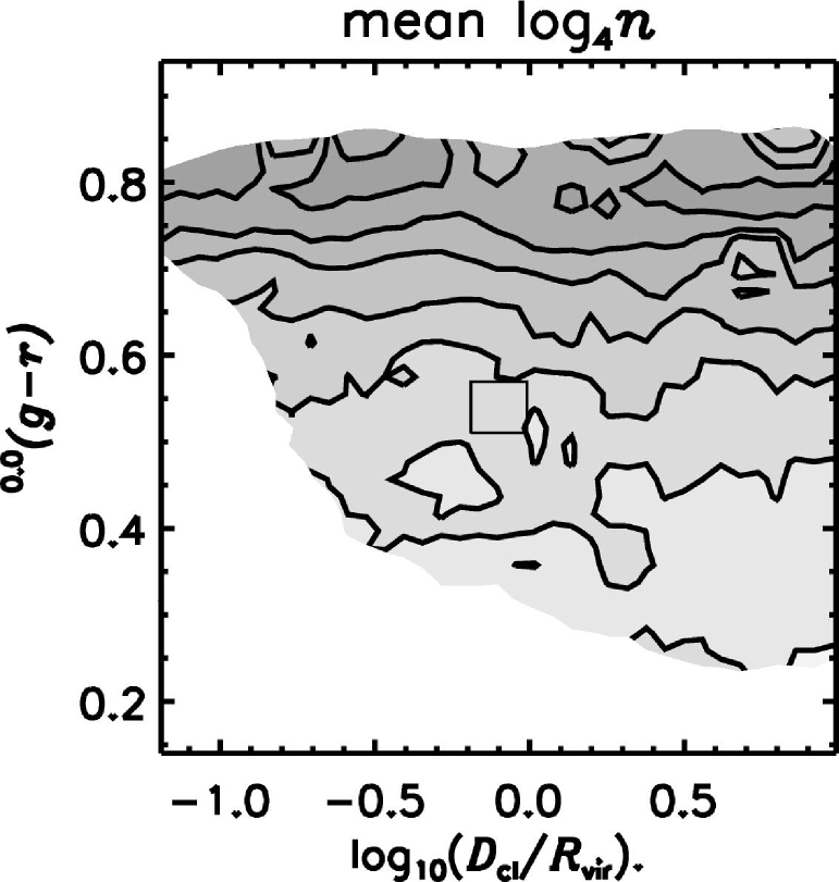
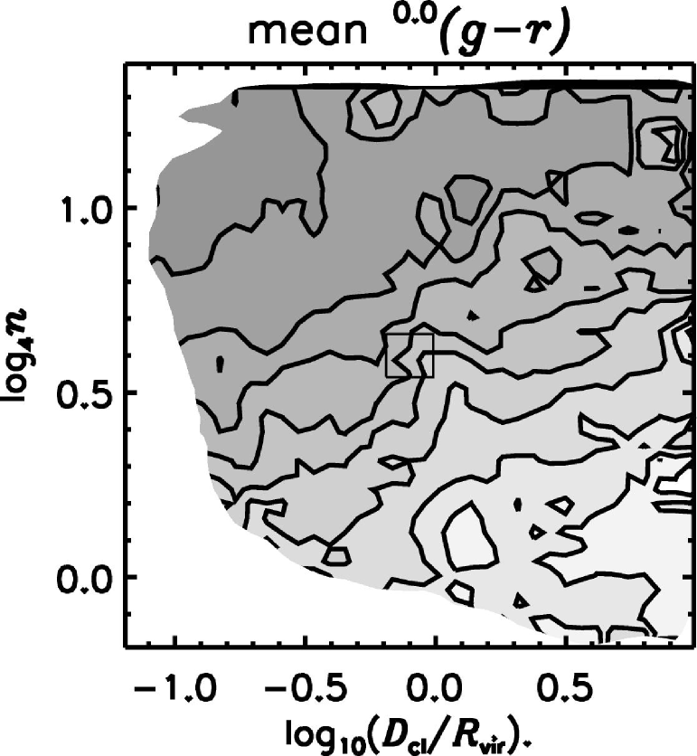
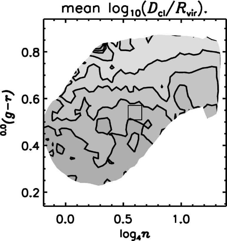
Figure 4: The left panel shows contours of mean radial concentration $n$ as a function of ${}^{0.0}[g-r]$ color and clustocentric distance $D_{\mathrm{cl}}$. The mean is computed in a sliding box shown in the center of the plot. The center panel shows contours of mean color as a function of concentration and clustocentric distance. The right panel shows contours of mean clustocentric distance as a function of color and concentration. Note that the contours in the left and right panels are more horizontal than the contours in the center panel.

Figure 4 displays the asymmetry shown in Figure 1 in a different way. The left panel shows that out of color and clustocentric distance, concentration depends only on color since the mean concentration contours are perpendicular to the color axis. The center panel shows that color depends on both concentration and clustocentric distance. The right panel shows that clustocentric distance depends more on color than concentration, since the contours are nearly perpendicular to the color axis.

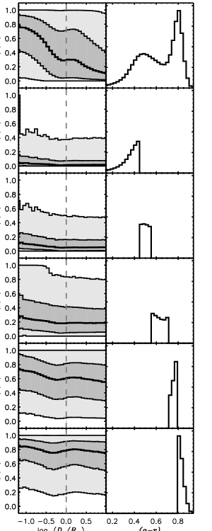
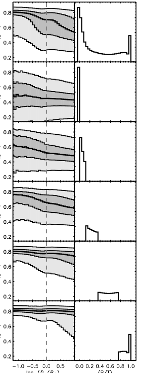
Figure 5: The same $2\times 6$ grids shown in Figure 1 but showing the Millennium simulation redshift zero outputs. Instead of concentration $n$ we show the ratio $B/T$ of the bulge luminosity to total luminosity as a morphology indicator. Notice the asymmetry seen in Figure 1 is not seen here.

Figure 5 is analogous to Figure 1 but showing the redshift zero outputs from the Millennium simulation. Instead of concentration $n$ we show the ratio of bulge luminosity to the total luminosity $B/T$. Notice that the asymmetry seen in the observed data is not reproduced here. The asymetry is also absent when we replace color with star-formation rate.

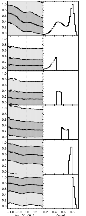
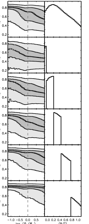
Figure 6: The same as Figure 5 but with thirty percent scatter (see text) added to the bulge-to-total values. Notice that the behavior of the trends do not significantly change when adding these large errors to $B/T$.

Figure 6 is the same as Figure 5 but with 30 percent random errors added to the $B/T$ values. The “random errors” were produced by randomly adding a Gaussian distribution with a dispursion of $\sigma=0.3$ to the Millennium $B/T$ values. Notice that the behavior of the trends do not significantly change when adding these large errors to $B/T$. This figure suggests that the asymmetry observed in the SDSS data is not due to the fact that we measure star-formation histories with much higher precision than we measure morphologies.

Another interesting result from Figures 1-3 is that the dependence of star-formation-history and morphological parameters on clustocentric distance is mostly limited to within the cluster virial radius. The top-left panels of these figures show that the trends observed at distances of less than the virial radius (denoted by the vertical dashed lines) nearly disappear at larger radii, where the relations between star-formation/morphological parameters and clustocentric distance are mostly flat. This result is not reproduced by the Millenium semi-analytic model. The top-left panels of Figure 5 show that, though the relations between model galaxy parameters and clustocentric radius flatten out near the virial radius, the strong trends resume at larger radii.

4 Summary and Discussion

Using a complete sample of 52,485 galaxies in the redshift range of $0.015<z<0.068$ we examine how star-formation history parameters—${}^{0.0}[g-r]$ color and $\mathrm{H}\alpha$ EW—and morphology parameters—radial concentration $n$ and surface brightness $\mu_{{}^{0.0}i}$—relate to environment. We use the transverse projected distance to the nearest cluster—the clustocentric distance $D_{\mathrm{cl}}$—as our environment parameter. Similar to Blanton et al. (2005a), we find that our morphology tracers (concentration and surface brightness) appear to be related to environment ($D_{\mathrm{cl}}$  in this case) only indirectly through their relationships with the star-formation history tracers. This suggests that the well known morphology–environment relation is a result of the star-formation-history–environment relation. We note that, although our simple morphology indicators do not show direct dependence on clustocentric distance, this result does not disagree with that the original morphology–density studies (Hubble, 1936; Oemler, 1974; Dressler, 1980; Postman & Geller, 1984) because these studies did not attempt to separate morphological and star-formation dependences. Our results also do not disagree with previous work (Vogt et al., 2004) which suggests that gas stripping plays a significant role in the morphological transformation and rapid truncation of star formation by showing asymmetries in HI and $\mathrm{H}\alpha$ flux on the leading edge of infalling spiral galaxies. There is no disagreement because our very blunt morphology indicators are insensitive to those asymmetries, and the asymmetries are only visible in a small fraction of all cluster galaxies.

Where our results overlap those of previous investigators (Christlein & Zabludoff, 2005; Blanton et al., 2005a), we mostly find good agreement. In particular, we find that galaxy properties depend on clustocentric distance in much the same way as they do on other environmental indicators (Blanton et al., 2005a). Our result improves on this previous one because the clustocentric distance is measured at much higher signal-to-noise and probes environments on scales much smaller than local overdensity measurements. Our results improve on the findings of Christlein & Zabludoff (2005) by reproducing their result with far higher signal to noise and by also by examining the inverse of their study. They found that star formation rate is related to environment independently of morphology. We find that both color and star formation rate behave in this way as well as that morphology doesn’t have a dependence on environment independent of star-formation history.

It is worth noting that this asymmetry may, in principle, be attributed to the measurements that were made instead of the properties of galaxies. This is possible because our star-formation-history properties are measured with far higher precision than our morphology properties. However, we do not believe this is true for two main reasons; (1) when we add large asymmetric noise to the Millennium bulge-to-total luminosities we still find no clear asymmetry and (2) the fact that we observe this asymmetry regardless of which star-formation history and morphology tracers we use, strongly suggests that it is a description of galaxy properties themselves. We stress that our main result, that there is no direct morphology–environment relation, holds for morphology defined by concentration and surface brightness. It remains untested whether other characterizations of morphology, such as spiral structure or asymmetry in the shape of the light distribution, also show this trait.

Our results also show that, where there are trends between galaxy properties and clustocentric distance, these trends are primarily restricted to within the cluster virial radii. This suggests that environmental processes that affect galaxy properties are fairly local (i.e., within the dark matter halo) and do not “act at a distance”. These results are not in agreement with those of Gomez et al. (2003) and Lewis et al. (2002) who found that there are trends out to $\sim 3$ times the virial radius. The discrepancy can be attributed to our different ways of estimating cluster virial radii. These authors use the Girardi et al. (1998) approximation relating virial radius to velocity dispersion, whereas we use virial radii based on the Berlind et al. (2006) mass estimates, which are derived from cluster abundances. We have checked the Girardi et al. (1998) approximation on our clusters and find that it yields virial radii that are $\sim 2$ times smaller than the ones we use, which explains much of the discrepancy. We trust our mass estimates because they are based on abundances, which have been shown to be unbiased for our clusters Berlind et al. (2006). Masses based on the Girardi et al. (1998) approximation yield an incorrect cluster mass function.

The asymmetry that we see between star-formation and morphological parameters has interesting implications for the role that environment plays in shaping galaxy properties. Our results suggest that environmental processes can affect galaxy star-formation histories without simultaneously affecting morphology, but in cases where an environmental mechanism does affect galaxy morphology, it must also affect star-formation history. Another possible explanation is that environment affects both star-formation history and morphology, but the changes in star-formation history occur on a much more rapid timescale than the corresponding changes to morphology.

In this short paper, we have investigated how galaxy star-formation histories and morphologies depend on environment. We find the following asymmetry: At fixed color, there is no dependence of morphology on environment, while at fixed morphology, there is a residual dependence of color on environment. This result suggests that the morphology–environment relation is a result of the combination of the star-formation-history–environment and the morphology–star-formation-history relations. Moreover, we performed a similar analysis on a semi-analytic model of galaxy formation and find that this asymmetry is not reproduced. Our results have important implications for the role that environment plays in shaping galaxy star-formation histories and morphology, and they place strong constraints on models of galaxy formation.

References

- Balogh et al. (2001) Balogh, M. L., Christlein, D., Zabludoff, A. I., & Zaritsky, D. 2001, ApJ, 557, 117
- Berlind et al. (2006) Berlind, A. A. et al. 2006, ApJS, 167, 1
- Blanton et al. (2003) Blanton, M. R., Brinkmann, J., Csabai, I., Doi, M., Eisenstein, D. J., Fukugita, M., Gunn, J. E., Hogg, D. W., & Schlegel, D. J. 2003, AJ, 125, 2348
- Blanton et al. (2005a) Blanton, M. R., Eisenstein, D., Hogg, D. W., Schlegel, D. J., & Brinkmann, J. 2005a, ApJ, 629, 143
- Blanton et al. (2003a) Blanton, M. R., Lin, H., Lupton, R. H., Maley, F. M., Young, N., Zehavi, I., & Loveday, J. 2003a, AJ, 125, 2276
- Blanton et al. (2003b) Blanton, M. R. et al. 2003b, ApJ, 594, 186
- Blanton et al. (2005b) Blanton, M. R. et al. 2005b, AJ, 129, 2562
- Christlein & Zabludoff (2005) Christlein, D. & Zabludoff, A. I. 2005, ApJ, 621, 201
- Croton et al. (2006) Croton, D. J. et al. 2006, MNRAS, 365, 11
- Dressler (1980) Dressler, A. 1980, ApJ, 236, 351
- Eisenstein et al. (2001) Eisenstein, D. J. et al. 2001, AJ, 122, 2267
- Fukugita et al. (1996) Fukugita, M., Ichikawa, T., Gunn, J. E., Doi, M., Shimasaku, K., & Schneider, D. P. 1996, AJ, 111, 1748
- Girardi et al. (1998) Girardi, M., Giuricin, G., Mardirossian, F., Mezzetti, M., & Boschin, W. 1998, ApJ, 505, 74
- Giuricin et al. (2001) Giuricin, G., Samurović, S., Girardi, M., Mezzetti, M., & Marinoni, C. 2001, ApJ, 554, 857
- Gomez et al. (2003) Gomez, P. et al. 2003, ApJ, 584, 210
- Gunn et al. (1998) Gunn, J. E., Carr, M. A., Rockosi, C. M., Sekiguchi, M., et al. 1998, AJ, 116, 3040
- Guzzo et al. (1997) Guzzo, L., Strauss, M. A., Fisher, K. B., Giovanelli, R., & Haynes, M. P. 1997, ApJ, 489, 37
- Hashimoto et al. (1998) Hashimoto, Y., Oemler, A., Lin, H., & Tucker, D. L. 1998, ApJ, 499, 589
- Hermit et al. (1996) Hermit, S., Santiago, B. X., Lahav, O., Strauss, M. A., Davis, M., Dressler, A., & Huchra, J. P. 1996, MNRAS, 283, 709
- Hogg (1999) Hogg, D. W. 1999, astro-ph/9905116
- Hogg et al. (2003) Hogg, D. W. et al. 2003, ApJ, 585, L5
- Hogg et al. (2004) Hogg, D. W. et al. 2004, ApJ, 601, L29
- Hubble (1936) Hubble, E. P. 1936, The Realm of the Nebulae (New Haven: Yale University Press)
- Kauffmann et al. (2004) Kauffmann, G., White, S. D. M., Heckman, T. M., Ménard, B., Brinchmann, J., Charlot, S., Tremonti, C., & Brinkmann, J. 2004, MNRAS, 314
- Kennicutt (1983) Kennicutt, R. C. 1983, AJ, 88, 483
- Lewis et al. (2002) Lewis, I. et al. 2002, MNRAS, 334, 673
- Lupton et al. (2001) Lupton, R. H., Gunn, J. E., Ivezić, Z., Knapp, G. R., Kent, S., & Yasuda, N. 2001, in ASP Conf. Ser. 238: Astronomical Data Analysis Software and Systems X, Vol. 10, 269
- Martínez et al. (2002) Martínez, H. J., Zandivarez, A., Domínguez, M., Merchán, M. E., & Lambas, D. G. 2002, MNRAS, 333, L31
- Norberg et al. (2002) Norberg, P. et al. 2002, MNRAS, 332, 827
- Oemler (1974) Oemler, A. 1974, ApJ, 194, 1
- Petrosian (1976) Petrosian, V. 1976, ApJ, 209, L1
- Pier et al. (2003) Pier, J. R., Munn, J. A., Hindsley, R. B., Hennessy, G. S., Kent, S. M., Lupton, R. H., & Ivezić, Ž. 2003, AJ, 125, 1559
- Postman & Geller (1984) Postman, M. & Geller, M. 1984, ApJ, 281, 95
- Quintero et al. (2004) Quintero, A. D. et al. 2004, ApJ, 602, 190
- Richards et al. (2002) Richards, G. et al. 2002, AJ, 123, 2945
- Schlegel et al. (1998) Schlegel, D. J., Finkbeiner, D. P., & Davis, M. 1998, ApJ, 500, 525
- Smith et al. (2002) Smith, J. A., Tucker, D. L., et al. 2002, AJ, 123, 2121
- Stoughton et al. (2002) Stoughton, C. et al. 2002, AJ, 123, 485
- Strateva et al. (2001) Strateva, I. et al. 2001, AJ, 122, 1861
- Strauss et al. (2002) Strauss, M. A. et al. 2002, AJ, 124, 1810
- Trujillo et al. (2002) Trujillo, I., Aguerri, J. A. L., Gutiérrez, C. M., Caon, N., & Cepa, J. 2002, ApJ, 573, L9
- Vogt et al. (2004) Vogt, N. P., Haynes, M. P., Giovanelli, R., & Herter, T. 2004, AJ, 127, 3300
- York et al. (2000) York, D. et al. 2000, AJ, 120, 1579
- Zehavi et al. (2005) Zehavi, I. et al. 2005, ApJ, 630, 1