Collective effects of stellar winds and unidentified gamma-ray sources

Abstract

We study collective wind configurations produced by a number of massive stars, and obtain densities and expansion velocities of the stellar wind gas that is to be target, in this model, of hadronic interactions. We study the expected $\gamma$-ray emission from these regions, considering in an approximate way the effect of cosmic ray modulation. We compute secondary particle production (electrons from knock-on interactions and electrons and positrons from charged pion decay), and solve the loss equation with ionization, synchrotron, bremsstrahlung, inverse Compton, and expansion losses. We provide examples where configurations can produce sources for GLAST satellite, and the MAGIC, HESS, or VERITAS telescopes in non-uniform ways, i.e., with or without the corresponding counterparts. We show that in all cases we studied no EGRET source is expected.

1 Single and collective stellar winds

LBL, WR, O and B stars lose a significant fraction of their mass in stellar winds with terminal velocities that can easily reach $V_{\infty}\sim 10^{3}$ km s^-1. With mass loss rates as high as $\dot{M}_{\star}=(10^{-6}-10^{-4})$ M_⊙ yr^-1, the density at the base of the wind can reach $10^{-12}$ g cm^-3 (e.g., 1 ). Such winds are permeated by significant magnetic fields, and provide a matter field dense enough as to produce hadronic $\gamma$-ray emission when pervaded by relativistic particles. A typical wind configuration (1 ; 2 ; 3 ) contains an inner region in free expansion (zone I) and a much larger hot compressed wind (zone II). These are finally surrounded by a thin layer of dense swept-up gas (zone III); the final interface with the interstellar medium (ISM). The innermost region size is fixed by requiring that at the end of the free expansion phase (about 100 years after the wind turns on) the swept-up material is comparable to the mass in the driven wave from the wind, which happens at a radius $R_{\rm wind}=V_{\infty}(3\dot{M}_{\star}/4\pi\rho_{0}V_{\infty}^{3})^{1/2}$, where $\rho_{0}\approx m_{p}n_{0}$ is the ISM mass density, with $m_{p}$ the mass of the proton and $n_{0}$ the ISM number density. After hundreds of thousands of years, the wind produces a bubble with a radius of the order of tens of parsecs, with a density lower (except that in zone I) than in the ISM. The matter in the inner region is described through the continuity equation: $\dot{M}_{\star}=4\pi r^{2}\rho(r)V(r)$, where $\rho(r)$ is the density of the wind and $V(r)=V_{\infty}(1-{R_{0}}/{r})^{\beta}$ is its velocity. $V_{\infty}$ is the terminal wind velocity, and the parameter $\beta$ is $\sim 1$ for massive stars (1 ). $R_{0}$ is given in terms of the wind velocity close to the star, $V_{0}\sim 10^{-2}V_{\infty}$, as $R_{0}=R_{\star}(1-(V_{0}/V_{\infty})^{1/\beta})$. Hence, the particle density is $n(r)=\dot{M}_{\star}(1-{R_{0}}/{r})^{-\beta}/({4\pi m_{p}V_{\infty}r^{2}}).$ In the case of a collection of winds, a hydrodynamical model taking into account the composition of different single stellar winds needs to be adopted. As we see below, differences with the single stellar wind case are notable.

Here we adopt a similar modelling to that of Cantó et al. (2000) 3 (see also 5 ; 6 ; 7 ) to describe the wind of a cluster (or a sub-cluster) of stars. Consider that there are $N$ stars in close proximity, uniformly distributed within a radius $R_{c}$, with a number density

$$n=\frac{3N}{4\pi R_{c}^{3}}\,.$$ (1)

Each star has its own mass-loss rate ($\dot{M}_{i}$) and (terminal) wind velocity ($V_{i}$), and average values can be defined as

$$\dot{M}_{w} = \frac{1}{N}\sum_{i}^{N}\dot{M}_{i}\,,$$ (2)

$$V_{w} = \left(\frac{\sum_{i}^{N}\dot{M}_{i}{V_{i}}^{2}}{N\,\dot{M}_{w}}\right)^{1/2}\,.$$ (3)

All stellar winds are assumed to mix with the surrounding ISM and with each other, filling the intra-cluster volume with a hot, shocked, collective stellar wind. A stationary flow in which mass and energy provided by stellar winds escape through the outer boundary of the cluster is established. For an arbitrary distance $R$ from the center of the cluster, mass and energy conservation imply that

$$\frac{4\pi}{3}R^{3}n\dot{M}_{w} = 4\pi R^{2}\rho V\,,$$ (4)

$$\frac{4\pi}{3}R^{3}n\dot{M}_{w}\left(\frac{1}{2}{V_{w}}^{2}\right) = 4\pi R^{2}\rho V\left(\frac{1}{2}{V}^{2}+h\right)\,,$$ (5)

where $\rho$ and $V$ are the mean density and velocity of the cluster wind flow at position $R$ and $h$ is its specific enthalpy (sum of internal energy plus the pressure times the volume),

$$h=\frac{\gamma}{\gamma-1}\frac{P}{\rho}\,,$$ (6)

with $P$ being the mean pressure of the wind and $\gamma$ being the adiabatic index (hereafter $\gamma=5/3$ to fix numerical values). From the mass conservation equation we obtain

$$\rho V=\frac{n\dot{M}_{w}}{3}R\,,$$ (7)

and the ratio of the two conservation equations imply

$$\frac{1}{2}V^{2}+h=\frac{1}{2}{V_{w}}^{2}\,.$$ (8)

The equation of motion of the flow is

$$\rho V\frac{dV}{dR}=-\frac{dP}{dR}-n\dot{M}_{w}V\,,$$ (9)

which, introducing the adiabatic sound speed $c$,

$$c^{2}=\gamma\frac{P}{\rho}\,,$$ (10)

can be written as

$$\rho V\frac{dV}{dR}=-\frac{1}{\gamma}\frac{d(\rho c^{2})}{dR}-n\dot{M}_{w}V\,.$$ (11)

From the definition of enthalpy and Equation (8), the adiabatic sound speed can be expressed as

$$c^{2}=\frac{\gamma-1}{2}({V_{w}}^{2}-V^{2})\,.$$ (12)

Using Equation (7), its derivative $d\rho$ and Equation (12) in (11) one obtains

$$\frac{dR}{R}=\frac{dV}{V}\left[\frac{(\gamma-1){V_{w}}^{2}-(\gamma+1)V^{2}}{(\gamma-1){V_{w}}^{2}+(5\gamma+1)V^{2}}\right]\,,$$ (13)

which can be integrated and expressed in more convenient dimensionless variables ($v\equiv V/V_{w}$ and $r\equiv R/R_{c}$) as follows

$$v\left[1+\frac{5\gamma+1}{\gamma-1}v^{2}\right]^{-(3\gamma+1)/(5\gamma+1)}=Ar\,,$$ (14)

with $A$ an integration constant. When $R>R_{c}$, i.e., outside the cluster, by definition $n=0$ and the mass conservation equation is

$$\dot{M}_{\rm assoc}\equiv\frac{4\pi}{3}{R_{c}}^{3}n\dot{M}_{w}=4\pi R^{2}\rho V\,,$$ (15)

where the middle equality gives account of the contribution of all stars in the association, and $\dot{M}_{\rm assoc}=\sum_{i}\dot{M_{i}}$ is the mass-loss rate at the outer boundary $R_{c}$. Substituting Equation (12) and (15) into the $n=0$ realization of Equation (11) one obtains

$$-\frac{dR}{R}=\frac{dV}{V}\left[\frac{(\gamma-1){V_{w}}^{2}-(\gamma+1)V^{2}}{2(\gamma-1)(V_{w}^{2}-V^{2})}\right]\,,$$ (16)

and integrating, the velocity in this outside region is implicitly defined from

$$v(1-v^{2})^{1/(\gamma-1)}=Br^{-2},$$ (17)

with $B$ an integration constant. Having constants $A$ and $B$ in Equations (14) and (17), see below, the velocity at any distance from the association center can be determined by numerically solving its implicit definitions, and hence the density is also determined, through Equation (7) or (15).

From Equation (17), two asymptotic branches can be found. When $r\rightarrow\infty$, either $v\rightarrow 0$ (asymptotically subsonic flow) or $v\rightarrow 1$ (asymptotically supersonic flow) are possible solutions. The first one (subsonic) produces the following limits for the density, the sound speed and the pressure

$$\rho_{\infty} = \frac{\dot{M}_{\rm assoc}}{4\pi B{R_{c}}^{2}V_{w}}\,,$$ (18)

$$c_{\infty}^{2} = \frac{\gamma-1}{2}{V_{w}}^{2}\,,$$ (19)

$$P_{\infty} = \frac{\gamma-1}{2\gamma}\frac{\dot{M}_{\rm assoc}V_{w}}{4\pi B{R_{c}}^{2}}\,.$$ (20)

If $P_{\infty}$ is the ISM pressure far from the association, the constant $B$ can be obtained as

$$B=\frac{\gamma-1}{2\gamma}\frac{\dot{M}_{\rm assoc}V_{w}}{4\pi P_{\infty}{R_{c}}^{2}}\,.$$ (21)

The velocity of the flow at the outer radius $r=1$ follows from Equation (17)

$$v_{r=1}(1-{v_{r=1}}^{2})^{1/(\gamma-1)}=B\,,$$ (22)

and continuity implies that

$$v_{r=1}\left[1+\frac{5\gamma+1}{\gamma-1}{v_{r=1}}^{2}\right]^{-(3\gamma+1)/(5\gamma+1)}=A\,.$$ (23)

Equation (14) implicitly contains the dependence of $v$ with $r$ in the inner region of the collective wind. Its left hand side is an ever increasing function. Thus, for the equality to be fulfilled for all values of radius (0$<r<$1), the right hand side of the equation must reach its maximum value at $r$=1. Deriving the right hand side of Eq. (14), one can find the velocity that makes it maximum

$$v_{\rm max}=\left(\frac{\gamma-1}{\gamma+1}\right)^{1/2}\,.$$ (24)

Since $v$ grows in the inner region, the maximum velocity is reached at $r=1$, and from Equation (22),

$$B=\left(\frac{\gamma-1}{\gamma+1}\right)^{1/2}\left(\frac{2}{\gamma+1}\right)^{1/(\gamma-1)}.$$ (25)

Continuity (Equation 23) implies that the value of $A$ is

$$A=\left(\frac{\gamma-1}{\gamma+1}\right)^{1/2}\left(\frac{\gamma+1}{6\gamma+2}\right)^{(3\gamma+1)/(5\gamma+1)}.$$ (26)

With the former value of $B$, and from Equation (21), if

$$P_{\infty}<\frac{1}{\gamma}\left(\frac{\gamma-1}{\gamma+1}\right)^{1/2}\left(\frac{\gamma+1}{2}\right)^{\gamma/(\gamma-1)}\frac{\dot{M}_{\rm assoc}V_{w}}{4\pi R_{c}^{2}}\,,$$ (27)

the subsonic solution is not attainable (continuity of the velocity flow is impossible) and the supersonic branch is the only physically viable. In this regime, the flow leaves the boundary of the cluster $R_{c}$ at the local sound speed $v_{\rm max}$ (equal to 1/2 for $\gamma=5/3$) and is accelerated until $v=1$ for $r\rightarrow\infty$.

Examples of the supersonic flow (velocity and particle density) for a group of stars generating different values of $\dot{M}_{\rm assoc}$, $V_{w}$, and $R_{c}$, are given in Table 1. The total mass contained up to 10 $R_{c}$ is also included in the Table as an example. A typical configuration of a group of tens of stars may generate a wind in expansion with a velocity of the order of 1000 km s^-1 and a mass between tenths and a few solar masses within a few pc (tens of $R_{c}$). We consider hadronic interactions with this matter.

Table 1: Examples of configurations of collective stellar winds. The mass is that contained within 10 $R_{c}$, and is shown as an example. $n_{0}$ is the central density.

Model	$\dot{M}_{\rm assoc}$	$V_{w}$	$R_{c}$	$n_{0}$	Wind mass
	[M⊙ yr-1]	[km s-1]	pc	cm-3	[M⊙ ]
A	$10^{-4}$	800	0.1	210.0	0.13
B	$10^{-4}$	800	0.3	23.3	0.39
C	$5\times 10^{-5}$	1000	0.2	20.9	0.11
D	$2\times 10^{-4}$	1500	0.4	13.9	0.56
E	$2\times 10^{-4}$	2500	0.2	33.5	0.17

However, it is to be noted that not all cosmic rays will be able to enter the collective wind. The difference between an inactive target, as that provided by matter in the ISM, and an active or expanding target, as that provided by matter in a single or a collective stellar wind, is indeed given by modulation effects. The cosmic ray penetration into the jet outflow depends on the parameter $\epsilon\sim VR/D$, where $V$ is velocity of wind, and $D$ is the diffusion coefficient. $\epsilon$ measures the ratio between the diffusive and the convective timescale of the particles (e.g., 8 ).

In order to obtain an analytic expression for $\epsilon$ for a particular star we consider that the diffusion coefficient within the wind of a particular star is given by (3 ; 8 ; 9 ) $D\sim\frac{1}{3}\lambda_{r}c,$ where $\lambda_{r}$ is the mean-free-path for diffusion in the radial direction (towards the star). The use of the Bohm parameterization seems justified, contrary to the solar heliosphere, since we expect that in the innermost region of a single stellar wind there are many disturbances (relativistic particles, acoustic waves, radiatively driven waves, etc.). In the case of a collective wind, the collision of individual winds of the particular stars forming the association also produce many disturbances. The mean-free-path for scattering parallel to the magnetic field ($B$) direction is considered to be $\lambda_{\|}\sim 10r_{g}=10E/eB$, where $r_{g}$ is the particle gyro-radius and $E$ its energy. In the perpendicular direction $\lambda$ is shorter, $\lambda_{\bot}\sim r_{g}$. The mean-free-path in the radial direction is then given by $\lambda_{r}={\lambda_{\bot}}^{2}\sin^{2}\theta+{\lambda_{\|}}^{2}\cos^{2}\theta=r_{g}(10\cos^{2}\theta+\sin^{2}\theta)$, where $\cos^{-2}\theta=1+(B_{\phi}/B_{r})^{2}$. Here, the geometry of the magnetic field for a single star is represented by the magnetic rotator theory (10 ; see also 1 ; 8 )

$$\frac{B_{\phi}}{B_{r}}=\frac{V_{\star}}{V_{\infty}}\left(1+\frac{R}{R_{\star}}\right)$$ (28)

and

$$B_{r}=B_{\star}\left(\frac{R_{\star}}{R}\right)^{2},$$ (29)

where $V_{\star}$ is the rotational velocity at the surface of the star, and $B_{\star}$ the surface magnetic field. Near the star the magnetic field is approximately radial, while it becomes tangential far from the star, where $\lambda_{r}$ is dominated by diffusion perpendicular to the field lines. This approximation leads —when the distance to the star is large compared with that in which the terminal velocity is reached, what happens at a few stellar radii— to values of magnetic field and diffusion coefficient normally encountered in the ISM.

Using all previous formulae,

$$E^{\rm min}(r)\sim\frac{3eB_{\star}V_{\infty}(r-R_{\star})}{c}\left(\frac{R_{\star}}{r}\right)^{2}\times\hskip 51.21504pt$$

$$\frac{\left(1+\left(\frac{V_{\star}}{V_{\infty}}\left(1+\frac{r}{R_{\star}}\right)\right)^{2}\right)^{3/2}}{10+\left(\frac{V_{\star}}{V_{\infty}}\left(1+\frac{r}{R_{\star}}\right)\right)^{2}}.$$ (30)

Equation (30) defines a minimum energy below which the particles are convected away from the wind. $E^{\rm min}(r)$ is an increasing function of $r$, the limiting value of the previous expression being

$$E^{\rm min}(r\gg R_{\star}) \sim \frac{3eB_{\star}V_{\infty}R_{\star}}{c}\left(\frac{V_{\star}}{V_{\infty}}\right)\sim 4.3\left(\frac{B_{\star}}{10{\rm G}}\right)\times$$ (31)

$$\left(\frac{V_{\star}}{0.1V_{\infty}}\right)\left(\frac{R_{\star}}{12{\rm R}_{\odot}}\right){\rm TeV}\,.$$

Therefore, particles that are not convected in the outer regions are able to diffuse up to its base. Note that $E^{\rm min}(r\gg R_{\star})$ is a linear function of all $R_{\star}$, $B_{\star}$ and $V_{\star}$, which is typically assumed as $V_{\star}\sim 0.1V_{\infty}$ (e.g., 1 ). There is a large uncertainty in these parameters, about one order of magnitude. The values of the magnetic field on the surface of O and B stars is under debate. Despite deep searches, only $5$ stars were found to be magnetic (with sizeable magnetic fields in the range of $B_{\star}\sim 100$ G) (e.g., 11 and references therein) typical surface magnetic fields of OB stars are then presumably smaller.

In the kind of collective wind, we consider that the collective wind behaves as that of a single star having a radius equal to $R_{c}$, and mass-loss rate equal to that of the whole association, i.e., $\dot{M}_{\rm assoc}$. The wind velocity at $R_{c}$, $V_{\star}$ is given by Equation (24). The order of magnitude of the surface magnetic field (i.e., the field at $R=R_{c}$) is assumed as the value corresponding to the normal decay of a single star field located within $R_{c}$, for which a sensitive assumption can be obtained using Equations (28) and (29), ${\cal O}(10^{-6}$) G. This results, for the whole association, in

$$[E^{\rm min}(r\gg R_{\star})]^{\rm assoc}\sim 0.8\left(\frac{B(R_{c})}{1\mu{\rm G}}\right)\left(\frac{R_{c}}{0.1{\rm pc}}\right){\rm TeV}.$$ (32)

The value of the magnetic field is close to that typical of the ISM, and should be consider as an average (this kind of magnetic fields magnitude was also used in modelling the unindentified HEGRA source in Cygnus, 12 ). In particular, if a given star is close to $R_{c}$ its contribution to the overall magnetic field near its position will be larger, but at the same time, its contribution to the opposite region (distant from it 2 $R_{c}$) will be negligible. In what follows we consider hadronic processes up to 10 – 20 $R_{c}$, so that a value of the magnetic field typical of ISM values is expected. We shall consider two realizations of $[E^{\rm min}(r\gg R_{\star})]^{\rm assoc}$, 100 GeV and 1 TeV.

2 $\gamma$-rays and secondary electrons from a cosmic ray spectrum with a low energy cutoff

The pion produced $\gamma$-ray emissivity is obtained from the neutral pion emissivity as described in detail in the appendix of 13 . For normalization purposes, we use the expression of the energy density that is contained in cosmic rays, $\omega_{\rm CR}=\int_{E}N(E)\,E\,dE$ and compare it to the energy contained in cosmic rays in the Earth environment, $\omega_{\rm CR,\oplus}(E)=\int_{E}N_{\oplus}(E)\,E\,dE$, where $N_{p\,\oplus}$ is the local cosmic ray distribution obtained from the measured cosmic ray flux. The Earth-like spectrum, $J_{\oplus}(E)$, is $2.2E_{{\rm GeV}}^{-2.75}$ cm^-2 s^-1 sr^-1 GeV^-1 (e.g. 12a ; 12b ), so that $\omega_{\rm CR,\oplus}(E>1{\rm GeV})\sim 1.5\,{\rm eVcm^{-3}}$. This implicitly defines an enhancement factor, $\varsigma$, as a function of energy

$$\varsigma(E)=\frac{\int_{E}N(E)\,E\,dE}{\omega_{\rm CR,\oplus}(E)}.$$ (33)

We assume that $N(E)$ is a power law of the form $N(E)=K_{p}E^{-\alpha}$. Values of enhancement $\gg 100$ at all energies are typical of star forming environments (see, e.g., 13 ; 14 ; 14b ; 17 ; 18 ; 19 ) and they would ultimately depend on the spectral slope of the cosmic ray spectrum and on the power of the accelerator. For a fixed slope, harder than that found in the Earth environment, the larger the energy, the larger the enhancement, due to the steep decline ($\propto E^{-2.75}$) of the local cosmic ray spectrum. In what follows, as an example, we consider enhancements of the full cosmic ray spectrum (for energies above 1 GeV) of 1000. With such fixed $\varsigma$, the normalization of the cosmic ray spectrum, $K_{p}$, can be obtained from Equation (33) for all values of the slope. Note that $K_{p}\propto\varsigma$, and thus the flux and $\gamma$-ray luminosity, $F_{\gamma}$ and $L_{\gamma}$, are linearly proportional to the cosmic ray enhancement. We compute secondary particle production (electrons from knock-on interactions and electrons and positrons from charged pion decay), and solve the loss equation with ionization, synchrotron, bremsstrahlung, inverse Compton and expansion losses (details are given in the papers 18 ; 20 ).

We now compute $\gamma$-ray fluxes in a concrete example, and following Section 1, we consider $\sim$2 M_⊙ of target mass being modulated within $\sim$1 pc. The average density is $\sim 25$ cm^-3. This amount of mass is typical of the configurations studied in Section previously within the innermost $20\,R_{c}\sim 2-8$ pc. To fix numerical values, we consider that the group of stars is at a Galactic distance of 2 kpc. Using the computations of secondary electrons and their distribution, we calculate the $\gamma$-ray flux when the proton spectrum has a slope of 2.3 and 2.0. In the latter case, to simplify, we show in Fig. 1 only the pion decay contribution which dominates at high energies, produced by the whole cosmic ray spectrum.

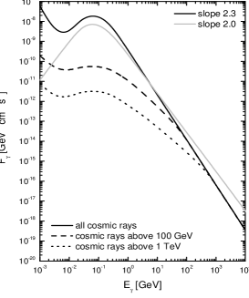
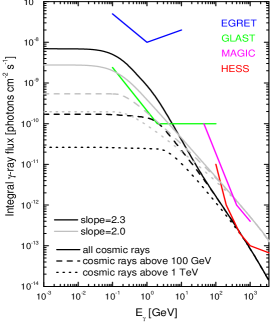
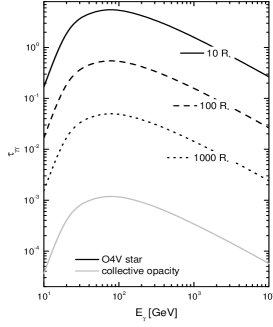
Figure 1: Differential (left) and integral (right) fluxes of $\gamma$-rays emitted in a non-modulated and a modulated environment. The bump at very low energies in the left panel is produced because we show leptonic emission coming only from secondary electrons. Above $\sim 70$ MeV the emission is dominated by neutral pion decay. Also shown are the EGRET, GLAST, MAGIC and HESS sensitivities. Note that a source can be detectable by IACTs and not by GLAST, or viceversa, depending on the slope of the cosmic ray spectrum and degree of modulation. Right: Opacities to $\gamma\gamma$ pair production in the soft photon field of an O4V-star at 10, 100 and 1000 $R_{\star}$, and in the collective photon field of an association with 30 stars distributed uniformly over a sphere of 0.5 pc. The closest star to the creation point is assumed to be at 0.16 pc, and the rest are placed following the average stellar density as follows: 1 additional star within 0.1, 2 within 0.25, 4 within 0.32, 8 within 0.40 and 14 within 0.5 pc.

The differential photon flux is given by $F_{\gamma}(E_{\gamma})=[{V}/{4\pi D^{2}}]{Q_{\gamma}(E_{\gamma})}=[{M}/{m_{p}\,4\pi D^{2}}][Q_{\gamma}(E_{\gamma})/n],$ where $V$ and $D$ are the volume and distance to the source, and $M$ the target mass. In those examples where the volume, distance and/or the medium density are such that the differential flux and the integral flux obtained from it above 100 MeV with the full cosmic ray spectrum is greater than instrumental sensitivity, a modulated spectrum with a 100 GeV or a 1 TeV energy threshold might not produce a detectable source in this energy range. However, the flux will be essentially unaffected at higher energy. The left panel of Fig. 1 shows that wind modulation can imply that a source may be detectable for the ground-based Cerenkov telescopes without even being close to be detected by instruments in the 100 MeV – 10 GeV regime (like EGRET or the forthcoming GLAST). The right panel of Fig. 1 presents the integral flux of $\gamma$-rays as a function of energy, together with the sensitivity of ground-based and space-based $\gamma$-ray telescopes. The sensitivity curves shown are for point-like sources; it is expected that extended emission would require about a factor of 2 more flux to reach the same level of detectability. Table 3 summarizes these results. From Table 3 and Fig. 1 we see that there are different scenarios (possible relevant parameters are distance, enhancement, degree of modulation of the cosmic ray spectrum and slope) for which sources that shine enough for detection in the GLAST domain may not do so in the IACTs energy range, and viceversa.

Finally, In Fig. 1 (rightmost panel) we show the value of the photon photon opacity, $\tau(E_{\gamma})$, for different photon creation sites distant from a O4V-star 10, 100, and 1000 $R_{\odot}$, with $R_{\star}=12R_{\odot}$ and $T_{\rm eff}=47400$ K. Unless a photon is created hovering the star, well within 1000 $R_{\star}$, $\gamma$-ray opacities are very low and can be safely neglected. This is still true for associations in which the number of stars is some tens. Consider for instance a group of 30 such stars within a region of 0.5 pc (the central core of an association). The stellar density is given by Eq. (1); and the number of stars within a circle of radius $R$ progresses as ${\cal N}=N(R/R_{c})^{3}$. Fig. 1 shows the collective contribution to the opacity in this configuration is also very low, since the large majority of the photons are produced far from individual stars. However, this is not the case if one considers the collective effect of a much larger association like the center of Cygnus OB 2 (21 ). Reimer demonstrated that even when a subgroup of stars like the ones considered here is separated from a super cluster like Cygnus OB2 by about 10 pc, the influence of the latter produces an opacity about one order of magnitude larger than that produced by the local stars. But even in this case, Fig. 1 shows that this opacity is not enough to preclude escape from the region of the local enhancement of stellar density.

3 Conclusions

We have studied collective wind configurations produced by a number of massive stars, and obtained densities and expansion velocities of the stellar wind gas that is target for hadronic interactions in several examples. We have computed secondary particle production, electrons and positrons from charged pion decay, electrons from knock-on interactions, and solve the appropriate diffusion-loss equation with ionization, synchrotron, bremsstrahlung, inverse Compton and expansion losses to obtain expected $\gamma$-ray emission from these regions, including in an approximate way the effect of cosmic ray modulation. Examples where different stellar configurations can produce sources for GLAST and the MAGIC/HESS/VERITAS telescopes in non-uniform ways, i.e., with or without the corresponding counterparts were shown. Cygnus OB 2 and Westerlund 1 maybe two associations where this scenario could be at work (20 ).

References

- (1) Lamers, H. J. G. L. M., & Cassinelli, J. P. 1999, Introduction to Stellar Winds, Cambridge University Press, Cambridge
- (2) Castor, J., McCray, R., & Weaver, R. 1975, ApJ, L107
- (3) Völk, H. J., & Forman, M. 1982, ApJ, 253, 188
- (4) Cantó J., Raga A. C. & Rodriguez L. F. 2000, ApJ 536, 896
- (5) Chevallier R. A. & Clegg A.W. 1975, Nature 317, 44
- (6) Ozernoy L. M., Genzel R. & Usov V. 1997, MNRAS 288, 237
- (7) Stevens I. R. & Hartwell J. M. 2003, MNRAS 339, 280
- (8) White R. L. 1985, ApJ, 289, 698
- (9) Torres D. F., Domingo-Santamaría, E., & Romero, G. E. 2004, ApJ 601, L75
- (10) Weber, E. J., & Davis, L. 1967, ApJ, 148, 217
- (11) Henrichs H. F., Schnerr R. S. & ten Kulve E. 2004, Conference Proceedings of the meeting: “The Nature and Evolution of Disks Around Hot Stars”, Johnson City, TN
- (12) Aharonian F. et al. 2005, A&A 431, 197
- (13) Aharonian F. 2001, Space Science Reviews 99, 187
- (14) Dermer, C. D. 1986, A&A, 157, 223
- (15) Domingo-Santamaría E. & Torres D. F. 2005, A&A 444, 403
- (16) Bykov, A. M., & Fleishman, G. D. 1992a, MNRAS, 255, 269
- (17) Bykov, A. M., & Fleishman, G. D. 1992b, Sov. Astron. Lett., 18, 95
- (18) Bykov, A. M. 2001, Space Sci. Rev., 99, 317
- (19) Torres D. F. et al. 2003, Phys. Rept. 382, 303
- (20) Torres D. F. 2004, ApJ 617, 966
- (21) Torres D. F. & Anchordoqui L. A. 2004, Rept. Prog. Phys. 67, 1663
- (22) Domingo-Santamaría E. & Torres D. F. 2006, A&A 448, 613
- (23) Reimer A. 2003, Proceedings of the 28th International Cosmic Ray Conference, p.2505