Cosmic microwave background and large-scale structure constraints on a simple quintessential inflation model

Abstract

We derive constraints on a simple quintessential inflation model, based on a spontaneously broken $\Phi^{4}$ theory, imposed by the Wilkinson Microwave Anisotropy Probe three-year data (WMAP3) and by galaxy clustering results from the Sloan Digital Sky Survey (SDSS). We find that the scale of symmetry breaking must be larger than about 3 Planck masses in order for inflation to generate acceptable values of the scalar spectral index and of the tensor-to-scalar ratio. We also show that the resulting quintessence equation-of-state can evolve rapidly at recent times and hence can potentially be distinguished from a simple cosmological constant in this parameter regime.

I Introduction

The inflationary scenario, in which the Universe undergoes a phase of accelerated expansion in its very early moments, provides an attractive solution to the flatness and horizon puzzles of the standard Big Bang cosmology. In addition, via quantum fluctuations, it naturally provides the seed perturbations for later structure formation in the Universe LindeBook . After inflation, reheating leads to a radiation-dominated era, followed by a more recent epoch in which the density is dominated by non-relativistic matter.

However, there is now solid observational evidence from Type Ia supernovae (SNIa) that the Universe is undergoing another burst of accelerated expansion; in the context of General Relativity, this must be fuelled by an unknown component with negative pressure, usually called dark energy (DE) Reviewdarkenergy .

The simplest possibility for the DE is the cosmological constant, $\Lambda$. Data from the cosmic microwave background (CMB) wmap , large-scale structure lss , and SNIa SNIaRiess ; SNIaLegacy are all consistent with the $\Lambda$CDM model, a nearly flat Universe with a cosmological constant and nearly scale-invariant primordial perturbations. In the best-fit $\Lambda$CDM model, the vacuum energy makes up 74$\%$ of the critical density, and the remainder is non-relativistic cold dark matter (CDM, 22$\%$) and baryonic matter (4$\%$).

While the cosmological constant is compatible with the current data, the recognition that the Universe appears to have undergone more than one period of accelerated expansion points to the plausibility of alternative explanations for the dark energy. In fact, there are no consensus particle physics models for either primordial inflation or the recent acceleration of the Universe. A first step out of our ignorance is often taken by introducing simple models, usually involving scalar fields. We can then proceed to test these models against data and obtain constraints on parameters that we hope can be calculated from a more fundamental theory. In this spirit, inflation and dark energy are often modelled via scalar fields, called the inflaton and the quintessence field.

In general, these two fields are treated as totally independent. In ref. us , we introduced a simple, well-motivated model that unifies these two fields into a single complex scalar field. We briefly review this model below.

We start with the general, renormalizable Lagrangian describing a complex scalar field $\Phi$; with appropriate choice of coupling constants, the associated global $U(1)$ symmetry is spontaneously broken at a high energy scale $f$ axions . The broken symmetry generates a flat potential for the phase of the complex field, $\varphi$, which at this stage is a massless Nambu-Goldstone boson. At a much lower energy scale, $M<<f$, instanton or other effects explicitly break the residual symmetry, providing a small mass for $\varphi$, now called a pseudo-Nambu Goldstone boson (PNGB). The QCD axion, a by-product of a solution to the strong CP problem, is an example of this phenomenon. PNGBs in the more general context are also sometimes called axions, a usage into which we shall lapse, but we emphasize that we are not here considering the QCD axion.

The resulting low-energy effective Lagrangian is given by:

$${\cal L}=\partial_{\mu}\Phi\partial^{\mu}\Phi^{\ast}-V(\Phi)+M^{4}[\cos(\mbox{Arg}(\Phi))-1]~{},$$ (1)

with the renormalizable potential

$$V(\Phi)=\lambda\left(\Phi\Phi^{\ast}-\frac{f^{2}}{2}\right)^{2}.$$ (2)

Writing the complex field $\Phi$ as

$$\Phi=\frac{1}{\sqrt{2}}\phi e^{i\varphi/f}$$ (3)

we identify the modular ($\phi$) and phase ($\varphi$) parts of $\Phi$ with the inflaton and the quintessence fields. A model in which the quintessence is such an axion-like PNGB field was introduced by Frieman et al. friemanetal . The model contains two mass scales, $f$ and $M$, and one dimensionless coupling constant, $\lambda$. As in the QCD case, we imagine that the lower scale $M$ is generated dynamically, by non-perturbative effects, leaving $f$ as the only fundamental mass scale in the theory. As is usually done, we have set the cosmological constant to zero.

In order for $\varphi$ to serve as dark energy, it must have not become dynamical until recently; otherwise, it would now be oscillating on a timescale short compared to the current Hubble time and would act instead as non-relativistic dark matter friemanetal . Therefore we require

$$m_{\varphi}=\frac{M^{2}}{f}\lesssim 3H_{0}$$ (4)

where $H_{0}=100\;h$ km/s/Mpc is the Hubble parameter today. On the other hand, for the energy density in the $\varphi$ field to have the correct order of magnitude to explain the acceleration, we must have

$$M^{4}\simeq\rho^{(0)}_{c}=\frac{3H_{0}^{2}M_{Pl}^{2}}{8\pi}.$$ (5)

Combining these two requirements results in friemanetal :

$$f>\frac{M_{Pl}}{\sqrt{24\pi}};\;\;\;\;M\simeq 3\times 10^{-3}\;h^{1/2}\;\mbox{eV},$$ (6)

where the Planck mass $M_{Pl}=1.2\times 10^{19}$ GeV.

This model was implemented in a hybrid inflation context by Massó and Zsembinszki MZ . A model similar to ours, in which the modulus field $\phi$ is responsible for inflation and the phase $\varphi$ produces dark matter, was studied in ref. KSY . In models in which the axion-like field is the dark matter, a high energy scale for the axion decay constant $f$ is also necessary, in order to suppress isocurvature fluctuations to acceptable levels. In our case, however, the axion field only becomes dynamical at such late times that the bounds from isocurvature fluctuations do not apply ByrnesWands .

II WMAP+SDSS constraints

The 3-year data set released by the WMAP collaboration (WMAP3) wmap has been used by a number of authors to constrain models of inflation AL ; KKMR ; SFK ; Cardoso . Of special interest to us are the reported limits on the scalar spectral index, $n_{s}$, and the ratio of tensor to scalar perturbations, $r$. Using WMAP3 plus the large-scale power spectrum of Luminous Red Galaxies (LRGs) in the Sloan Digital Sky Survey (SDSS), Tegmark, et al. Tegmarketal derive the marginalized constraints:

$$n_{s}=0.967^{+0.022}_{-0.020}\;;\;\;\;r<0.33\;(@\;95\%\;\mbox{CL}).$$ (7)

Note that the above constraints were obtained in the context of the $\Lambda$CDM model, i.e., assuming that the dark energy equation of state is $w=-1$, and also assuming spatial flatness, massless neutrinos, and no running of the scalar spectral index with spatial wavelength, but allowing for non-zero tensor perturbations. Dropping one or more of those assumptions would weaken the constraints.

As shown in Fig. 19 of Tegmarketal (reproduced below in Fig. 1), under the assumptions above, a simple chaotic $\lambda\phi^{4}$ inflationary model is marginally excluded at 95 % CL by the WMAP3+SDSS constraints. Since our proposed inflation model approaches a $\lambda\phi^{4}$ potential at large values of $\phi$, one might worry that it is also disfavored by current data. We will see below that this is not the case in general; rather, values of the fundamental mass parameter $f$ below a certain level are excluded.

In this model, inflation is driven by the modulus field $\phi$, since the potential energy associated with $\varphi$ is smaller by $\sim 112$ orders of magnitude. The potential $V(\Phi)$ in Eq.(2) in fact depends only on $\phi$,

$$V(\phi)=\frac{\lambda}{4}\left(\phi^{2}\ -f^{2}\right)^{2}.$$ (8)

Working in the context of the slow-roll approximation, where the field evolution is slow ($\ddot{\phi}\simeq 0$, $\dot{\phi}\simeq-V^{\prime}/(3H)$), we can define the usual slow-roll parameters $\epsilon$ and $\eta$ inflation :

$$\epsilon\left(\phi\right) = {M_{Pl}^{2}\over 16\pi}\left({V^{\prime}\left(\phi\right)\over V\left(\phi\right)}\right)^{2};$$ (9)

$$\eta\left(\phi\right) = {M_{Pl}^{2}\over 8\pi}\left[{V^{\prime\prime}\left(\phi\right)\over V\left(\phi\right)}-{1\over 2}\left({V^{\prime}\left(\phi\right)\over V\left(\phi\right)}\right)^{2}\right].$$ (10)

Slow roll is a consistent approximation for $V^{\prime},\ V^{\prime\prime}\ll V$ (in Planck units) or equivalently for $\epsilon,\ \eta\ll 1$. In particular, inflation ends when $\epsilon\simeq 1$.

In our case we find

$$\epsilon\left(\phi\right) = {M_{Pl}^{2}\over\pi}{\phi^{2}\over\left(\phi^{2}-f^{2}\right)^{2}};$$ (11)

$$\eta\left(\phi\right) = {M_{Pl}^{2}\over 2\pi}{1\over\left(\phi^{2}-f^{2}\right)}.$$ (12)

Defining $\phi_{e}$ as the value of the field $\phi$ at the end of inflation, $\epsilon\left(\phi_{e}\right)=1$ we find two possible solutions:

$$\left(\phi_{e}\right)^{2}=f^{2}+{M_{Pl}^{2}\over 2\pi}\left(1\pm\sqrt{1+4\pi f^{2}/M_{Pl}^{2}}\right).$$ (13)

The solution with positive sign has $|\phi_{e}|>f$ and corresponds to large-field inflation; that is, the field starts at $|\phi_{i}|>|\phi_{e}|>f$ and slowly rolls to values close to $f$ until inflation stops. The solution with negative sign has $|\phi_{e}|<f$ and corresponds to small-field inflation: the field starts near the local maximum at $|\phi_{i}|<|\phi_{e}|<f$ and slowly rolls to values closer to $f$ until the end of inflation.

The number $N$ of e-folds remaining until the end of inflation in terms of the value of the field $\phi_{N}$ required to accomplish this number of e-folds is given by:

$$N={\sqrt{4\pi}\over M_{Pl}}\int_{\phi_{e}}^{\phi_{N}}{d\phi\over\sqrt{\epsilon(\phi)}}={\pi\over M_{Pl}^{2}}\left(\phi_{N}^{2}-\phi_{e}^{2}-f^{2}\ln\left(\phi_{N}^{2}/\phi_{e}^{2}\right)\right).$$ (14)

There is a bound on the maximum number of e-folds between the time that the present Hubble radius leaves the horizon and the end of inflation. The bound derives from limits on the gravitational wave background (provided that the energy density of the Universe does not drop faster than that of radiation after inflation) and is given roughly by $N_{\mbox{max}}\simeq 60$ DH ; LL . In the following we will use $N=50$ and $60$ for illustration and denote the corresponding field value by $\phi_{N}$.

Once we solve Eq. (14) for $\phi_{N}$, we can immediately compute the spectral index of perturbations, $n_{s}$, and the ratio of tensor to scalar perturbations, $r$ KKMR :

$$n_{s,N} = 1-4\epsilon\left(\phi_{N}\right)+2\eta\left(\phi_{N}\right)$$ (15)

$$r_{N} = 16\epsilon\left(\phi_{N}\right)$$ (16)

Table 1: Large-field Inflation: For different values of the vacuum expectation value $f$, we show the value of the scalar field ($\phi_{50}$, $\phi_{60}$) when the present Hubble radius crosses outside the horizon and at the end ($\phi_{e}$) of inflation, all in units of the Planck mass. $n_{N}$ and $r_{N}$ denote the corresponding values of the scalar spectral index and the tensor-to-scalar ratio.

$f$	$\phi_{e}$	$\phi_{50}$	$\phi_{60}$	$n_{50}$	$n_{60}$	$r_{50}$	$r_{60}$
0.1	0.581	4.04	4.41	0.941	0.951	0.313	0.262
1.0	1.32	4.48	4.84	0.946	0.955	0.280	0.237
3.0	3.40	6.17	6.49	0.954	0.961	0.229	0.195
5.0	5.29	8.06	8.37	0.956	0.963	0.207	0.176

In Table 1, we show the resulting values for $n_{s,N}$ and $r_{N}$ for different values of the symmetry breaking scale $f$, for the large-field case, $|\phi_{i}|>f$. For $f<M_{Pl}$, we have $\phi>>f$ throughout inflation; in this limit, the potential of Eqn.(8) is close to that of a pure $\lambda\phi^{4}$ theory, and the resulting values of $n_{s}$ and $r$ are similar to those of the $\phi^{4}$ model. For larger values of $f$, $\phi_{e}/f$ is close to unity; in this regime, one can expand the potential during inflation around $\phi=f$ and find that it is closer to quadratic than quartic. For $f~{}\hbox to0.0pt{$>$\hss}{\lower 4.30554pt\hbox{$\sim$}}\;3M_{Pl}$, Fig.1 shows that the resulting values of $n_{s}$ and $r$ are consistent with the $68\%$ limits from WMAP3+SDSS LRG for values of $N$ approaching 60.

At 95% CL, the parameter range $f>1M_{Pl}$ is allowed by the current data.

Figure 1: Regions in the $r$ vs. $n_{s}$ plane excluded by WMAP1 (in red), WMAP3 (in beige), and by WMAP3+SDSS (in yellow), from Tegmarketal . The two contours in the white region show those allowed at 68% and 95% CL. Regions occupied by chaotic inflation models with $\phi^{2}$, $\phi^{4}$, and $\phi^{6}$ potentials are indicated. We have superimposed regions occupied by our model in the large-field regime for $f=1,3$, and $5M_{Pl}$ (black, dashed) and in the small-field regime for $f=2,3$, and $5M_{Pl}$ (green, dot-dashed). Moving down these curves, the number of e-folds before the end of inflation that the Hubble radius expands outside the horizon varies from $N=50$ to 60 (except for the $\phi^{4}$ case, in which $N=64$ was used).

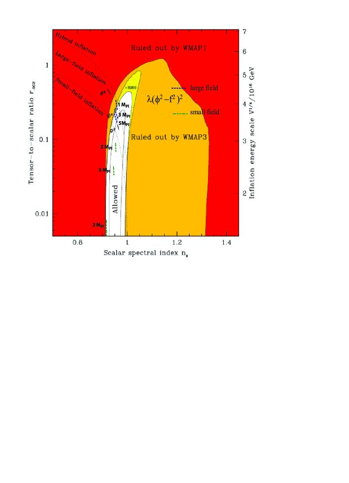
Results for the case of small-field inflation, $|\phi_{i}|<f$, are shown in Table 2. In this case, one can expand the potential around $\phi=0$, resulting in $V(\phi)\propto f^{4}(1-2\phi^{2}/f^{2})$. For $f~{}\hbox to0.0pt{$<$\hss}{\lower 4.30554pt\hbox{$\sim$}}\;M_{Pl}$, $\phi_{60}$ is exponentially smaller than $\phi_{e}$ KM , which is unnatural, especially since quantum fluctuations impose a lower bound on the field amplitude. In fact, for $f<0.8M_{Pl}$, we find no solutions to Eqn. (14) in the small-field case. In this regime, for $\phi_{60}\ll f$, one finds $n_{s}\simeq M_{Pl}^{2}/(\pi f^{2})$. As $f$ increases, there is a transition at $f\simeq M_{Pl}$, where the scalar spectral index gets substantialy closer to 1. As shown in Fig.1, consistency with WMAP3+SDSS at 68% CL requires $f~{}\hbox to0.0pt{$>$\hss}{\lower 4.30554pt\hbox{$\sim$}}\;3M_{Pl}$.

From Tables 1 and 2 and Eqns.(11,12), we see that $\epsilon(\phi_{N}),\eta(\phi_{N})\ll 1$ for most of the cases studied, validating the use of the slow-roll approximation.

The fact that the symmetry-breaking scale $f$ must be near $M_{Pl}$ is potentially appealing from the theoretical point of view, since the latter is a fundamental mass scale of gravitational origin. However, the observational constraint that $f$ must be several times larger than the Planck mass could raise concern about the validity of the semi-classical field theory approach and about the possibility of large gravitational corrections to the theory that could destroy the requisite flatness of the scalar field potential. In this context, we note that models with two twoaxions or more moreaxions axions have been proposed, in which a linear combination can result in an effective scale $f$ larger than $M_{Pl}$ while the fundamental mass scales in the theory are below the Planck mass.

Table 2: Small-field Inflation: For different values of the vacuum expectation value $f$, we show the value of the scalar field ($\phi_{50}$, $\phi_{60}$) when the present Hubble radius crosses outside the horizon and at the end ($\phi_{e}$) of inflation, all in units of the Planck mass. $n_{N}$ and $r_{N}$ denote the corresponding values of the scalar spectral index and the tensor-to-scalar ratio.

$f$	$\phi_{e}$	$\phi_{50}$	$\phi_{60}$	$n_{50}$	$n_{60}$	$r_{50}$	$r_{60}$
1.0	0.757	$0.0002$	$0.00004$	0.682	0.682	0.0	0.0
2.0	1.74	0.163	0.110	0.918	0.919	0.00862	0.00385
3.0	2.73	0.770	0.639	0.951	0.956	0.0428	0.0282
5.0	4.73	2.49	2.29	0.961	0.967	0.0893	0.0686

III Thawing the quintessence field

It is interesting to study the consequences of this constraint on the symmetry breaking energy scale $f$ for the quintessence PNGB field in our model, described by the Lagrangian

$${\cal L}=\frac{1}{2}(\partial_{\mu}\varphi)^{2}-M^{4}[1-\cos(\varphi/f)].$$ (17)

The quintessence behaviour is determined by three parameters, $f$, $M$, and the initial value $\varphi_{i}$ of the field when it was dynamically frozen in the early Universe. Once we fix values of two of the parameters, for instance $f$ and $M$, the value of $\varphi_{i}$ is determined by requiring that $\Omega_{\varphi}\simeq 0.7$ today. Since $\varphi$ only became dynamical at late times, the parameter $M^{4}$ must be of the order of the critical density today, cf. Eqn.(5), or larger. The steepness of the quintessence potential is measured by the mass of the $\varphi$ field, $m_{\varphi}\simeq M^{2}/f$. The larger the mass of the field, the earlier it can evolve, and therefore the larger the deviations of its equation of state from that of a cosmological constant, $w=-1$. We show this behaviour in figure 2 by numerically solving the equations of motion for $\varphi$. We fix $f=5$ $M_{Pl}$, in keeping with the WMAP+SDSS constraints, and simultaneously vary $M$ and $\varphi_{i}$ to keep $\Omega_{\varphi}=0.7$ today, following quint . We see that the PNGB quintessence equation of state $w(z)$ can evolve significantly at recent times for large values of $M^{4}$, making it distinct from a simple cosmological constant, as emphasized recently in the context of the so-called see-saw cosmology seesaw . For fixed $f$, the value of $M$ is bounded from below by the requirement that the quintessence field energy be large enough to dominate the Universe today and from above by the requirement that it drive accelerated rather than decelerated expansion. As pointed out in friemanetal ; seesaw , one can achieve evolution of the sort shown in Fig. 2 without fine-tuning the mass parameters of the model. Such behavior is consistent with current constraints on the evolution of $w(z)$ (see, e.g., draganhiranya ) but could be tested by future projects aimed at probing the dark energy.

Figure 2: Evolution of the quintessence equation of state parameter $w(z)$ as a function of redshift for $f=5$ $M_{Pl}$, $\Omega_{\varphi}=0.7$, and $M^{4}=10(5.4),30(3.2),50(2.5)$, and $100(1.8)$ times $\rho^{(0)}_{c}$ (from bottom to top curves). The numbers in parentheses are the initial values of the field $\varphi_{i}$ in Planck mass units for the corresponding value of $M$.

IV Conclusions

In this Brief Report, we have studied the constraints on a simple model of quintessential inflation previously proposed by us us that arise from the WMAP3 CMB and SDSS LRG data. We find that the effective scale of symmetry breaking, $f$, must be larger than about 3 $M_{Pl}$ in order to satisfy the constraints on the scalar spectral index and the tensor-to-scalar ratio from inflation. With these constraints, the resulting quintessence equation of state parameter $w(z)$ can nevertheless evolve rapidly at recent times, $z~{}\hbox to0.0pt{$<$\hss}{\lower 4.30554pt\hbox{$\sim$}}\;1-2$, depending on the value of the induced explicit symmetry breaking scale $M$, an example of a ‘thawing’ dark energy model. Such models can be tested by precision probes of the dark energy equation of state expected over the coming decade.

References

- (1) See, e.g., A. D. Linde, Inflation and Quantum Cosmology, Academic Press (1990).
- (2) For reviews on dark energy, see e.g., P. J. E. Peebles and B. Ratra, Rev. Mod. Phys. 75, 559 (2003); T. Padmanabhan, Phys. Rept. 380, 235 (2003); E. J. Copeland, M. Sami, S. Tsujikawa, hep-th/0603057.
- (3) D. N. Spergel et al., Astrophys. J. Supp. 148, 175 (2003), astro-ph/0302209 and astro-ph/0603449
- (4) See, e.g., K. Abazajian et al., Astron. J. 126, 2081 (2003).
- (5) A. G. Riess et al., Astrophys. J. 607, 665 (2004).
- (6) P. Astier et al., Astron. Astrophys. 447, 31 (2006).
- (7) R. Rosenfeld and J. A. Frieman, JCAP 09, 003 (2005).
- (8) R. D. Peccei and H. Quinn, Phys. Rev. Lett. 38, 1440 (1977); S. Weinberg, Phys. Rev. Lett. 40, 223 (1978); F. Wilczek, Phys. Rev. Lett. 46, 279 (1978).
- (9) J. A. Frieman, C. T. Hill, A. Stebbins and I. Waga, Phys. Rev. Lett. 75, 2077 (1995).
- (10) E. Massó and G. Zsembinszki, JCAP 0602, 012 (2006).
- (11) M. Kawasaki, N. Sugiyama and T. Yanagida, Phys. Rev. D54, 2442 (1996).
- (12) C. T. Byrnes and D. Wands, Phys. Rev. D73, 063509 (2006).
- (13) L. Alabidi and D. H. Lyth, JCAP 0608, 013 (2006).
- (14) W. H. Kinney, E. W. Kolb, A. Melchiorri and A. Riotto, Phys. Rev. D74, 023502 (2006).
- (15) C. Savage, K. Freese and W. H. Kinney, astro-ph/0609144.
- (16) A. Cardoso, astro-ph/0610074.
- (17) M. Tegmark et al., astro-ph/0608632.
- (18) For a review see, e.g., D. H. Lyth and A. Riotto, Phys. Rept. 314, 1 (1999).
- (19) S. Dodelson and L. Hui, Phys. Rev. Lett. 91, 131301 (2003).
- (20) A. R. Liddle and S. M. Leach, Phys. Rev. D68, 103503 (2003).
- (21) W. H. Kinney and K. T. Mahanthappa, Phys. Rev. D53, 5455(1996).
- (22) J. E. Kim, H. P. Nilles and M. Peloso, JCAP 0501, 005 (2005).
- (23) N. Kaloper and L. Sorbo, JCAP 0604, 007 (2006); S. Dimopoulos, S. Kachru, J. McGreevy, J. G. Wacker hep-th/0507205; P. Svrcek, hep-th/0607086.
- (24) U. França and R. Rosenfeld, JCAP 0210, 015 (2002).
- (25) L. J. Hall, Y. Nomura and S. J. Oliver, Phys. Rev. Lett. 95, 141302 (2005).
- (26) D. Huterer and H. Peiris, astro-ph/0610427.