Swift and XMM-Newton Observations of the Extraordinary GRB 060729: More than 125 days of X-ray afterglow

Abstract

We report the results of the Swift and XMM-Newton observations of the Swift-discovered long Gamma-Ray Burst GRB 060729 ($T_{90}$=115s). The afterglow of this burst was exceptionally bright in X-rays as well as at UV/Optical wavelengths showing an unusually long slow decay phase ($\alpha$=0.14$\pm$0.02) suggesting a larger energy injection phase at early times than in other bursts. The X-ray light curve displays a break at about 60 ks after the burst. The X-ray decay slope after the break is $\alpha$=1.29$\pm$0.03. Up to 125 days after the burst we do not detect a jet break, suggesting that the jet opening angle is larger than 28^∘. In the first 2 minutes after the burst (rest frame) the X-ray spectrum of the burst changed dramatically from a hard X-ray spectrum to a very soft one. We find that the X-ray spectra at this early phase can all be fitted by an absorbed single power law model or alternatively by a blackbody plus power law model. The power law fits show that the X-ray spectrum becomes steeper while the absorption column density decreases. In the blackbody model we find that the temperature changes from $kT=0.6$ keV at 85 s after the burst to 0.1 keV at 160 s after the burst in the rest frame. In Swift’s UV/Optical telescope the afterglow was clearly detected up to 9 days after the burst in all 6 filters and even longer in some of the UV filters with the latest detection in the UVW1 31 days after the burst, which is one of the latest detections of an afterglow by the UVOT. A break at about 50 ks is clearly detected in all 6 UVOT filters from a shallow decay slope of about 0.3 and a steeper decay slope of 1.3. The spectral energy distributions show that there is no spectral development between X-rays and the UV/optical throughout the observation. In addition to the Swift observations we also present and discuss the results from a 61 ks Target-of-Opportunity observation by XMM-Newton starting about 12 hours after the burst. These observations show a typical afterglow X-ray spectrum with $\beta_{\rm X}$=1.1 and absorption column density of $1\times 10^{21}$ cm^-2.

1 Introduction

Gamma-Ray Bursts (GRBs) are the most powerful explosions in the present-day Universe. With the launch of the Swift Gamma-Ray Burst Explorer Mission (Gehrels et al., 2004) in November 2004 a new era in GRB science has started. Swift is able to observe the afterglow of a burst with its narrow-field instruments, the X-ray Telescope (XRT, Burrows et al., 2005a) and the UV/Optical telescope (UVOT; Roming et al., 2005), typically within 2 minutes after the detection by the Burst Alert Telescope (BAT, Barthelmy et al., 2005). Several phenomena were discovered by Swift, like the occurrence of giant flares during the first 1000 s after the burst (e.g. Burrows et al., 2005b; Falcone et al., 2006) or the canonical light curves of GRB afterglows (Nousek et al., 2006; Zhang et al., 2006).

GRB 060729 was discovered by Swift on 2006 July 29 (Grupe et al., 2006) as one of the brightest bursts ever detected in X-rays by Swift (With the brightest GRB in XRT so far being GRB 061121; Page et al., 2007). Besides GRB 050525A (Blustin et al., 2005), GRB 060218 (Campana et al., 2006), GRB 060614 (Mangano et al., in preparation, ), and GRB 061121 (Page et al., 2007), GRB 060729 is the burst with the best UVOT follow up even up to 9 days after the burst in all 6 UVOT filters and even longer in some of the UV filters. In the XRT the afterglow has been detected by more than 125 days after the burst. This is the longest follow-up observation with a detection of an afterglow ever performed by Swift. Similar coverage, but shorter, has only been performed for GRBs 050416A, 060319, and 060614. Even though the burst was bright in the BAT, it was too faint to be detected by Konus-Wind (Frederiks, priv. comm.).

Even though the sun angle was small in RA (2.2 h), due to the declination of Dec=–62^∘ the afterglow was circumpolar for most southern observatories, and was observed by the ESO VLT using FORS2 and by Gemini South using GMOS (Thoene et al., 2006). A redshift of z=0.54 was determined from the optical spectra by Thoene et al. (2006). GRB 060729 was also observed by ROTSE IIIa, located at the Siding Spring Observatory, Australia, by Quimby et al. (2006), who reported an initial upper limit of 16.6 mag 64 s after the BAT trigger. They were able to detect the afterglow with ROTSE IIIa up to 175 ks after the burst when it was still at 19.4 mag (Quimby & Rykoff, 2006), decaying with a slope $\alpha$=0.23. Cobb & Bailyn (2006) measured a decay slope in the I band of $\alpha_{\rm I}$=1.5 based on CTIO 1.3m SMARTS observations between 4.6 to 17.6 days after the burst.

The paper is organized as follows: In §2 we describe the observations and the data reduction. In §3 we present the data analysis. The discussion of our results is given in §4. Throughout the paper decay and energy spectral indices $\alpha$ and $\beta$ are defined by $F_{\nu}(t,\nu)\propto(t-t_{0})^{-\alpha}\nu^{-\beta}$, with $t_{0}$ the trigger time of the burst. Luminosities are calculated assuming a $\Lambda$CDM cosmology with $\Omega_{\rm M}$=0.27, $\Omega_{\Lambda}$=0.73 and a Hubble constant of $H_{0}$=71 km s^-1 Mpc^-1 using the luminosity distances $D_{\rm L}$ given by Hogg (1999) resulting in $D_{\rm L}$=3120 Mpc. All errors are 1$\sigma$ unless stated otherwise.

2 Observations and data reduction

The Swift BAT triggered on the pre-cursor of GRB 060729 at 19:12:29 UT on 2006 July 29 (Grupe et al., 2006; Grupe, 2006). Swift’s X-ray Telescope began observing the afterglow 124 s after the trigger. The UVOT started the observations 135 s after the BAT trigger.

The Swift XRT observed GRB 060729 in the Windowed Timing (WT) and Photon Counting (PC) observing modes (Hill et al., 2004). The XRT data were reduced by the xrtpipeline task version 0.10.4. The WT mode data at the beginning of the XRT observation had to be treated with special care. During the first 20s after the start (130–150s after the BAT trigger) of the WT XRT observation the satellite was still settling causing the target to move on the XRT CCD towards the dead columns at DETX=319–321 (Abbey et al., 2006). In order to correct for the photon losses due to these dead columns we measured the offset of the source at each second and calculated a correction factor according to the losses of the WT mode Point Spread Function (PSF). After 150s after the trigger all WT mode data were corrected by the same factor. Source and Background photons were selected by XSELECT version 2.4 in boxes with a length of 40 pixel. For count rates $>$ 150 counts s^-1, however, in the WT mode the data had to be corrected for pileup. In order to correct for pileup in the light curve and for the spectral analysis and the determination of the hardness ratio we excluded the central regions of the PSF at the source position depending on the count rate as described in Romano et al. (2006). For the PC mode data the source photons were selected in a circular region with a radius of r=59${}^{{}^{\prime\prime}}$ and the background photons in a circular region close by with a radius r=176${}^{{}^{\prime\prime}}$ in the first segments. For the later data the radii were reduced to 47${}^{{}^{\prime\prime}}$ and 24${}^{{}^{\prime\prime}}$ for the source, and 137${}^{{}^{\prime\prime}}$ and 96${}^{{}^{\prime\prime}}$ for the background. For the spectral data only events with grades 0–2 and 0–12 were selected with XSELECT for the WT and PC mode data, respectively. Note that the source photons for the spectral analysis of the PC mode data of the first orbit were selected in a ring with an inner radius of $16\farcs 5$ and an outer radius of $71\farcs 0$ in order to avoid the effects of pile-up (e.g. Pagani et al., 2006; Vaughan et al., 2006). The spectral data were re-binned by using grppha version 3.0.0 having 20 photons per bin. The spectra were analyzed with XSPEC version 12.3.0 (Arnaud, 1996). The auxiliary response files were created by xrtmkarf and corrected using the exposure maps, and the standard response matrices swxwt0to2_20010101v008.rmf and swxpc0to12_20010101v008.rmf were used for the WT and PC mode data, respectively. All spectral fits were performed in the observed 0.3–10.0 keV energy band. For the errors of the spectral fit parameters we used the standard $\Delta\chi^{2}$=2.7 in XSPEC, that is equivalent to a 90% confidence region for a single parameter.

Background-subtracted X-ray flux light curves in the 0.3–10.0 keV energy range of the Swift observations were constructed using the ESO Munich Image Data Analysis Software MIDAS (version 04Sep) and by an IDL program that corrects for PSF losses, in particular when the source is located on one of the dead columns on the XRT CCD detector. The light curve was binned as follows: the WT mode data with 1000 photons per bin, and the pc mode data with 200 counts per bin in the first days after the burst and 20 or 10 at the end of the observations. The count rates were converted into unabsorbed flux units using energy conversion factors (ECF) which were determined by calculating the count rates and the unabsorbed fluxes in the 0.3–10.0 keV energy band using XSPEC as described in Nousek et al. (2006). The XRT data at the beginning of the observation show dramatic spectral changes and require specific ECFs for each time bin. The later data, however, do agree with a typical afterglow spectrum and the count rates were converted by one ECF=5$\times 10^{-11}$ ergs s^-1 cm^-2 (counts s^-1)^-1.

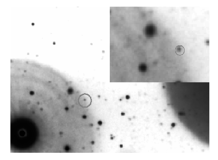
Figure 1: UVW1 image ($5\farcm 7\times 4\farcm 2$) of the field of GRB 060729 with an exposure of 550 ks. The circles at the source position displays the XRT position as given in Section 3.1. The circles in the large image show a 8${}^{{}^{\prime\prime}}$ radius at the source just for display purposes, and the 8${}^{{}^{\prime\prime}}$ background extraction region. The zoom-in image (80${}^{{}^{\prime\prime}}\times 60^{{}^{\prime\prime}}$) in the upper right corner shows the $3\farcs 5$ XRT error radius. Note the bright star which is only 107${}^{{}^{\prime\prime}}$ away from the position of the afterglow of GRB 060729.

The Swift UVOT observations of GRB060729 began with the automated “GRB” sequence, which provided finding chart images in White (100 s) and V (400 s), then began cycling through all 6 UV and optical filters starting 739 s after the trigger. The source data of these early White and V images were extracted from a circle with a radius of 6${}^{{}^{\prime\prime}}$. GRB 060729 remained detectable in all 6 filters for more than 9 days after the trigger, then for 12 days after the trigger in UVW2 ($\lambda_{c}=1930$Å) and for 31 days after the trigger in UVW1 ($\lambda_{c}=2510$Å). During the first days after the burst each observation in each single orbit was analyzed. For the later data the images were coadded with uvotimsum in order to improve the signal to noise ratio. The data were analyzed with the UVOT software tool uvotsource. Due to the bright F3V star HD 45187 (9.4 mag in B, 107$\farcs$5 away from GRB 060729) extra caution had to be taken for the source extraction and the background subtraction. We chose a selection radius of 4${}^{{}^{\prime\prime}}$ for the source and $8^{{}^{\prime\prime}}$ for the background in all filters placed at a position nearby on the rim of the bright star’s halo as displayed in Figure 1. In order to correct for losses due to this small source extraction radius, we did an aperture correction with V=0.03 mag, B=0.05 mag, U=0.05 mag, UVW1=0.17 mag, UVM2($\lambda_{c}=2170$Å)=0.15 mag, and UVW2=0.15 mag. All values plotted and listed in this paper take these corrections into account. The data, however, are not corrected for Galactic reddening, which is $E_{\rm B-V}$=0.050 mag (Schlegel et al., 1998) in the direction of the burst.

GRB 060729 was also observed by XMM-Newton (Jansen et al., 2001) for a total of 61 ks (Schartel, 2006; Campana & De Luca, 2006). XMM-Newton started observing the afterglow of GRB 060729 on 2006 July 30 07:41 (44.9 ks after the trigger) to 2006 July 31 01:04 UT (107.5 ks after the trigger). In the European Photon Imaging Camera (EPIC) pn (Strüder et al., 2001) the total observing time was 59.6 ks using the medium light blocking filter. However, due to high particle background during part of the observation only 42.3 ks were used. The observations in the EPIC MOS (Turner et al., 2001) were for a total observing time of 61.2 ks. The MOS1 was using the medium filter while the MOS2 observations were performed with the thin filter. The total observing time in the Reflection Grating Spectrometers (RGS; den Herder et al., 2001) was 61.5 ks. In the Optical Monitor (OM; Mason et al., 2001) the afterglow was observed for 8.3 ks in U, 5$\times$ 4 ks in UVW1, 3$\times$ 4 ks in UVM2, and 2$\times$ 4 ks with the optical grism. Note, that the OM UVW1 and UVM2 filters are slightly different compared with the UVOT UV filters. The XMM-Newton data were reduced with the latest SAS version xmmsas_20060628_1801-7.0.0.

3 Data Analysis

3.1 Position of the Afterglow

The position of the afterglow measured from the UVOT UVW1 coadded image is
RA (J2000) = $06^{\rm h}21^{\rm m}31\fs 86$,
Dec (J2000) = $-62^{\circ}22^{\prime}12\farcs 5$
with a 1${}^{{}^{\prime\prime}}$ error. This position is consistent with the initial analysis of the White and V filter analysis (Immler, 2006). The UVW1 position is $1\farcs 1$ away from the X-ray position RA (J2000) = $06^{\rm h}21^{\rm m}31\fs 75$, Dec (J2000) = $-62^{\circ}22^{\prime}13\farcs 3$ (with a $3\farcs 5$ 90% confidence error), which was measured for the XRT PC mode data of segment 001 using the new teldef file swx20060402v001.teldef as described in Burrows et al. (2006a). This position deviates by $3\farcs 2$ from the refined position given in Grupe (2006). The most likely reason for this difference is that for the X-ray position given in Grupe (2006) only the PC mode data of the first orbit were used. This is due to the burst during the first orbit being placed on one of the bad columns on the XRT CCD which makes the determination of a position difficult. Figure 1 displays the UVW1 image of the field of GRB 060729. The circle in the upper right inserted image is the $3\farcs 5$ XRT error radius of the X-ray position given above.

3.2 BAT data

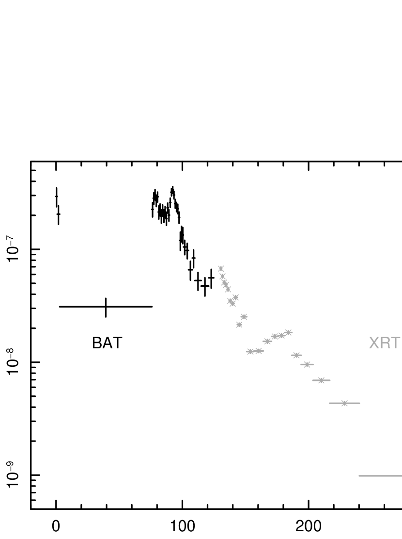
Figure 3: Combined Swift BAT and XRT WT light curves. The Figure clearly shows that the XRT was starting observing GRB 060729 during the fourth peak seen in the BAT.

Figure 2 displays the BAT light curves in the 15–25 keV, 25–50 keV, 50–100 keV, and 15– 100 keV bands (top to bottom) with $T_{0}$= 2006 July 29 19:12:29 UT (Spacecraft clock 175893150.592). GRB 060729 had a $T_{90}$=115s (Parsons et al., 2006). Partly the $T_{90}$ is so long because the trigger was on the pre-cursor. After the initial first peak (pre-cursor) which was detected by the BAT and which triggered the observation the burst drops back down to the background level. However, two giant peaks are observed at about 60s after the trigger, of which the first one is harder than the second. There is a third peak which peaks about 120s after the trigger. This is the peak of which we see the end of the decay in the XRT (Figure 3). For the spectral analysis the BAT data were divided into 5 bins as listed in Table 1. The first peak is the initial peak the BAT triggered on GRB 060729. As shown in Table 1, the following two peaks that occur between 70 and 124s after the burst are by a factor of 3 stronger than the initial peak. The two last peaks (124-190s after the burst, XRT flare 1 and 2 in Table 1) are also observed simultaneously in the XRT. These data will be discussed in the XRT section.

Table 1 lists the results of the spectral analysis of the 5 peaks. All spectra were fitted by a single power law model. The initial peak has a hard spectrum with a 15–150 keV energy spectra index $\beta_{\rm 15-150keV}$=1.05${}^{+0.42}_{-0.32}$. The two strong peaks between 70–124s after the burst show an interesting spectral behavior. While the first of these peaks (70-88s after the burst) has a rather hard spectral slope with $\beta_{\rm 15-150keV}$=0.59$\pm$0.11, the second of these peaks (88-124s) was softer with $\beta_{\rm 15-150keV}$=0.90$\pm$0.11. The total fluence in the observed 15-150 keV band is 2.7$\times 10^{-6}$ ergs cm^-2 (Parsons et al., 2006) and 7.2$\times 10^{-6}$ ergs cm^-2 and 1.7$\times 10^{-5}$ ergs cm^-2 in the rest-frame 1 keV – 1 MeV and 1 keV – 10 MeV bands, respectively, adding all BAT spectra together (Table 1) and assuming the same power law spectrum as in the 15-150 keV band without any break. With the redshift z=0.54 this converts into an isotropic energy in the rest-frame 1 keV - 1 MeV and 1 keV – 10 MeV band of $E_{\rm iso}=6.7\times 10^{51}$ ergs and $E_{\rm iso}=1.6\times 10^{52}$ ergs, respectively. Because we lack observations of the break energy $E_{\rm break}$ and the $\gamma$-ray spectrum at higher energies by Konus-Wind the 1 keV – 10 MeV band $E_{\rm iso}$ value is an upper limit of the true isotropic energy.

3.3 X-ray data

3.3.1 Temporal analysis

Figure 3 shows the combined BAT and XRT light curve. The light curve clearly shows that XRT began observing the GRB at the beginning of the fourth peak seen in the BAT. The combined BAT + XRT light curve was constructed as described in O’Brien et al. (2006). Due to the dramatic spectral change within the three minutes of the WT observation, we applied an ECF for each individual bin assuming power law model corrected for absorption with the parameters listed in Table 2. However, for the BAT data we applied only one ECF that reflects the main spectrum.

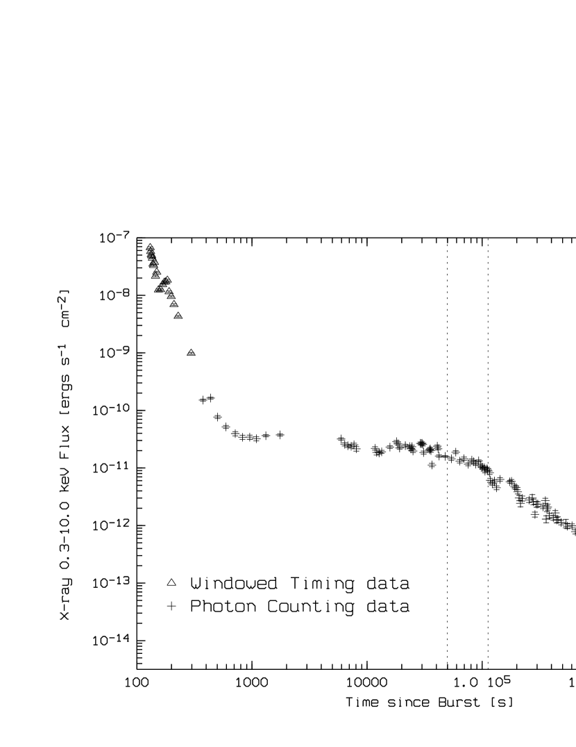
Figure 4: Swift XRT light curve of the Windowed Timing (triangles) and photon counting (crosses). The downward arrow marks the 3$\sigma$ upper limit at the end of the Swift observations. This upper limit contains a total exposure time of 63.5 ks obtained between 2006 December 8 and December 27. The dotted vertical lines mark the start and end times of the XMM-Newton observation.

Figure 4 displays the Swift XRT light curve, with WT mode data as triangles and PC mode data as crosses. The vertical dashed lines in the figure mark the start and end times of the XMM-Newton observations. The general behavior of the light curve can be described as follows: after the initial steep decay with a decay slope $\alpha_{\rm 1}$ = 5.11$\pm$0.22 the light curve flattens at $T_{\rm break,1}$ = 530s$\pm$25s with a decay slope $\alpha_{\rm 2}$ = 0.14$\pm$0.02. At $T_{\rm break,2}$ = 56.8 ks$\pm$10ks the light curve of the afterglow breaks again and continues decaying with a decay slope $\alpha_{\rm 3}$ = 1.29$\pm$0.03. The definitions of the decay slopes follow the descriptions given in Nousek et al. (2006) and Zhang et al. (2006). We do not detect a jet break even 125 days after the burst. The last 3$\sigma$ detection of the X-ray afterglow was obtained between 2006 November 21 to December 01 with a total exposure time of 69.9 ks. The afterglow was still observed by Swift until December 27 for a total of 63.5 ks. However these observations were interrupted by several new bursts and at the end only a 3$\sigma$ upper limit of 2.1$\times 10^{-14}$ ergs s^-1 cm^-2 could be obtained. It was dropped from the Swift schedule after 2006 December 27 because it was not detectable anymore with the XRT within a reasonable amount of observing time.

3.3.2 Spectral Analysis

Dramatic spectral change at the beginning

In order to examine the spectral behavior in more detail, source and background spectra were created for each bin, except for the first 10 bins ($T-T_{0}$=130–150 s). The WT mode data were divided into 21 bins with 1000 source photons in each bin. Because of the high count rate at the beginning of the observations we applied the method as described in Romano et al. (2006) to avoid the effects of pileup. However, this procedure reduced significantly the number of source photons in each single spectrum. We, therefore, combined two bins into one for bins 1+2, 3+4, 5+6, 7+8, and 9+10 to increase the signal to noise ratio.

Each of the 16 spectra were fitted by an absorbed single power law, blackbody plus power law, and a power law with exponential cutoff model. The results of these spectral fits are listed in Table 2. Figure 5 shows plots of the WT mode data; from top to bottom the count rate, hardness ratio, the X-ray spectral slope $\beta_{\rm X}$ from an absorbed single powerlaw fit with a free fit absorption column density $N_{H}$, blackbody temperature kT (in keV) from the blackbody plus power law fit, the blackbody radius $R_{\rm bb}$ and the break energy $E_{\rm break}$ of a power law with exponential cutoff model. The hardness ratio changes from HR=0.6 at the beginning of the observation to HR=$-$0.56 at the end, indicating a dramatic evolution in the X-ray spectrum within 2 minutes of observing time which translates into 1.3 minutes in the rest frame.

While the spectra during the first 20 s of the WT mode observation are well-fitted by a single power law model, after about 150s after the burst the data are better fit by a blackbody plus power law spectrum. For the absorbed power law fits, all parameters were left free. We found that while the spectra at the beginning of the observation were rather hard with $\beta_{\rm X}$=1.5 and $N_{\rm H}$=$4\times 10^{21}$ cm^-2, the spectra became very soft with $\beta_{\rm X}$$\sim$3.0 and $N_{\rm H}$=$1\times 10^{21}$ cm^-2. Note that the absorption column density $N_{\rm H}$ decreases while the energy spectral index $\beta_{\rm X}$ becomes steeper - the opposite than what is expected if the spectral slope and the absorption column density were just linked in the fitting program. However, note that especially during the later bins, the spectra are not well fit by a single power law and do require more complicated models.

For the blackbody plus power law model, the absorption parameter was fixed to the Galactic value (4.82$\times 10^{20}$ cm^-2 Dickey & Lockman, 1990) and the hard energy spectral slope to $\beta_{\rm X}$=1.0. The blackbody temperature changes dramatically from $kT$=0.56 keV at the beginning of the XRT WT observation to 0.11 keV at the end, accompanied by an increase of the blackbody radius from 2.5$\times 10^{12}$ cm to 16$\times 10^{12}$ cm. Fitting the data with an absorbed blackbody plus power law model with the absorption column density at z=0 set to the Galactic value and at z=0.54 set to $1\times 10^{21}$ cm^-2 (see the discussion about the XMM-Newton spectral analysis) results in similar values for the temperature. The only differences are that the temperatures tend to be lower by 40 eV and the normalizations are higher.

The prompt emission of GRBs is often fitted by a Band function (Band et al., 1993). We also tried a power law model with exponential cutoff, which is a surrogate for the Band model, which has the advantage of using fewer parameters than the Band model. In order to obtain better constraints we fixed the absorption column to the Galactic value. As listed in Table 2, typically the power law model with exponential cutoff does not show improvements over the single power law or the blackbody plus power law models.

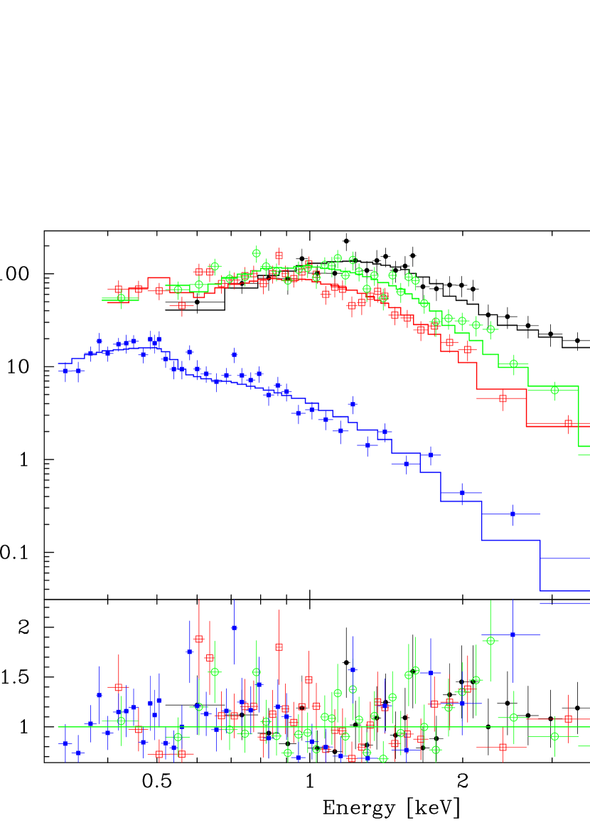
Figure 6: Swift XRT WT spectra of bins 1+2 (black filled circles), 12 (red open squares), 14 (green open circles), and 21 (blue filled squares) fitted by absorbed single power laws as given in Table 2. The numbers refer to the bins as shown in Figure 5.

The change in the X-ray spectra is also displayed in Figure 6 which shows the spectra of bins # 1, 12, 14, and 21. Bin 12 is the bin before the small flare at 170s after the burst and bin 14 is the peak of that flare.

Later PC mode data

All PC mode data can be fitted by a power law model with a energy spectral slope $\beta_{\rm X}$=1.2 and an absorption column density of about 1.5$\times 10^{21}$ cm^-2. This absorption column density is significantly above the Galactic value . The intrinsic absorption column density at the redshift z=0.54 is 1.9$\pm$0.4$\times 10^{21}$ cm^-2. Table 3 lists the XRT PC mode observations at 20–40 ks after the burst and at 200 ks after the burst, so before and after the XMM observation. The fits to these data suggest no significant spectral variability before and after the break in the X-ray light curve around 60 ks after the burst.

The XMM-Newton observations

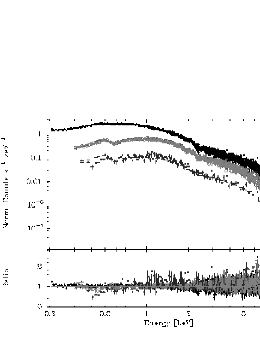
Figure 7: Absorbed power law model fits with $N_{\rm H}$=8.57$\times 10^{20}$ cm^-2 and $\beta_{\rm X}$=1.08, as listed in Table 3, to the XMM-Newton EPIC pn (black filled circles), MOS1 (red open squares), MOS2 (green open circles), and Swift XRT PC mode(blue filled squares) spectra. The Swift XRT data were selected between 44.9 ks to 107.5 ks after the burst, simultaneous with the XMM-Newton observation.

The combined spectra of the XMM-Newton EPIC pn and MOS and Swift XRT data are shown in Figure 7. The XRT data were selected between 44900 s and 107500 s after the burst. The details of the spectral fits to these data are summarized in Table 3. At these late times, the X-ray spectra were well fitted by absorbed single power law models. However, as a check the spectra were fitted also by a blackbody plus power law model, but at these late times the power law component dominates the spectra. Therefore, we will only discuss the absorbed power law model fits as listed in Table 3.

The obvious difference between the Swift XRT and XMM-Newton pn and MOS data is the much higher value of the absorption column density. From the free fit absorption column density at z=0 we measured an absorption column density $N_{\rm H}$=15.7$\times 10^{20}$ cm^-2 in the Swift XRT data. This value is about twice as high as what is measured from the XMM-Newton EPIC pn and MOS spectra. The EPIC pn is well-calibrated to energies below 0.2 keV (e.g. Haberl et al., 2003). We also applied the gain fit model within XSPEC, but it did not remove the discrepancy. This discrepancy maybe due to problems with the Swift XRT bias maps during the time period 2006 July 21 and 2006 August 3. This bias map problem causes an offset in the gain and therefore compromises the spectral analysis of Swift XRT PC mode data during that time period. However, this gain shift does not affect the early Swift XRT WT mode data. Due to the better response of the EPIC pn at lower energies we consider the absorption column densities measured by the EPIC pn the most reliable. With the redshift of the burst at z=0.54 we can also use the X-ray spectra to determine the intrinsic absorption column density at the location of the afterglow. The intrinsic column densities of all fits are in the order of $1\times 10^{21}$ cm^-2, except for the Swift XRT data which again show an absorption column density about twice as high. As we will show later in section 3.5 the absorption column density of $1\times 10^{21}$ cm^-2 is in good agreement to what can be derived from the spectral energy distribution of the afterglow.

In addition to the EPIC pn and MOS data we also analyzed the 2 RGS spectra. We found that the analysis of the RGS continuum spectra agrees within the errors with the pn and MOS data. We did not find any obvious emission or absorption features in the RGS spectra.

3.4 UV/Optical data analysis

The magnitudes resulting from the UVOT data analysis are listed in Table 4. Figure 8 shows the results of the UVOT photometry in comparison with the XRT. UVOT was able to follow the afterglow in all six filters up to 9 days after the burst. In UVW1 the afterglow was followed up 31 days after the burst which translates into 20 days in the rest-frame. This is one of the longest intervals Swift’s UVOT has ever detected an afterglow in the optical/UV. Only GRBs 060218 (Campana et al., 2006) and 060614 (Mangano et al., in preparation, ) were detected at slightly later observed times than GRB 060729.

In all bands, XRT as well as in all 6 UVOT filters, a significant break occurs in the light curve. Table 5 lists the decay slopes $\alpha_{\rm 2}$ and $\alpha_{\rm 3}$ before and after the break time $T_{\rm break}$. Within the errors all break times seem to occur at about 50 ks after the burst (33 ks in the rest-frame), with the earliest break in B at about 30ks and the later breaks at shorter wavelengths. However, considering the uncertainties in the decay slopes, this is all consistent with an achromatic break. Note that due to a rebrightening of the afterglow at about 20 ks seen in X-rays and all 6 UVOT filters the determination of $\alpha_{2}$ is rather uncertain. In B the afterglow decays the slowest with $\alpha_{3}$=0.98. The decay slopes at shorter wavelengths are steeper with $\alpha_{3}\approx$=1.3. Note that the flatter slope in the B-Filter is caused by a re-brightening at about 200 ks that is not seen in the other filters. By limiting the analysis to data only up to 200ks the decay slope is $\alpha_{3}$=1.17$\pm$0.16 which is consistent with the decay slopes seen in the other filters. The rebrightening in B at about 200 ks after the burst seems to be real. We checked for any strong variability in the background but could not detected any strong background variation at that time. The decay slopes $\alpha_{2}$ and $\alpha_{3}$ are consistent with the decay slopes reported by Quimby & Rykoff (2006) and Cobb & Bailyn (2006).

Figure 9 displays the UVOT White and V and XRT light curves of the first orbit. The UVOT data of this period are listed in Table 6. The left panel of Figure 9 displays the UVOT White filter event mode and XRT WT mode data. The UVOT White filter data were grouped into 10 s bins. The first UVOT White points show a decay similar to the XRT WT light curve. However after these few points the UVOT White light curve flattens, which agrees with the flare seen in the XRT data at 170s after the burst. At about 200s after the burst the afterglow starts to become brighter in the UVOT White, while it is still decaying in X-rays.

The right panel of Figure 9 shows the UVOT V event mode data and the XRT PC mode data of the first orbit. The UVOT V data were grouped in 25 s bins and the XRT PC mode data with 25 source photons per bin. The UVOT V light curve shows the afterglow fairly constant at about 17.5 mag while the XRT PC mode light curves shows an initial decay until about 600s and flattens after that.

The XMM-Newton Optical Monitor observations are summarized in Table 7. While the U filter results agree well with the UVOT U data as listed in Table 4, there is a discrepancy in the UVW1 and UVM2 filters. There maybe two explanations for this discrepancy: 1) The OM and UVOT UV filter sets have different filter transmission, 2) OM suffers from significantly higher level of scattered light than the UVOT, and third the extraction radius of the automated OM software is 12${}^{{}^{\prime\prime}}$ which is too large for an accurate analysis of the UV data due to the bright star (see UVOT section). The brightening of the afterglow in the last OM UVM2 observation at 101 ks after the burst is most likely due to a bad subtraction of the background within the automatic OM data reduction software.

3.5 Spectral Energy Distribution

As shown in section 3.4 the long-term light curves in all 6 UVOT filters and in X-rays do follow the same decay slope with similar break times at about 50 ks after the burst. In order to check this we determined spectral energy distributions (SEDs) of the afterglow at 800s, 20 ks, 100 ks, and 500 ks, with exposure times in the XRT of 400s, 1.8 ks, 3.3 ks, and 4.8 ks, respectively. Figure 10 displays these four SEDs. These times are also marked in Figure 8. These times were picked to represent the SEDs of the earliest and latest time possible when the afterglow was detected in all 6 UVOT filters and shortly before and after the break. All fluxes in all 6 UVOT filters and the XRT were calculated according to the light curves. There seem to be no obvious changes in the SEDs, besides the changes in the fluxes, over time. Another measure of any changes in the SEDs over time is the optical/UV to X-ray spectral slope or X-ray loudness $\beta_{\rm ox}$. For the afterglow of GRB 060729 we measured rest-frame $\beta_{\rm ox}$ of 0.85$\pm$0.10 at 800s, 0.84$\pm$0.05 at 20 ks, 0.74$\pm$0.07 at 100 ks, and 0.77$\pm$0.10 at 500 ks after the burst. Within the errors these values are consistent and do not suggest any changes between the optical/UV and X-ray parts of the SED over time after the first orbit. However, note that during the first $\approx$400s of data the SED changes dramatically, because the X-ray flux decays very fast ($\alpha_{x,1}$=5.1 while the White and V data suggest that the optical afterglow is constant. A single power law spectrum between optical/UV and X-ray energies a $\beta_{\rm ox}$=1.1 is expected according to the fits to the X-ray data (Table 3). This assumption of a single power law spectrum between the optical and X-rays is justified given that the optical has the same temporal behavior as the X-rays and that the optical and X-rays are both above the cooling frequency. The difference between the expected $\beta_{\rm ox}$=1.1 and the measured $\beta_{\rm ox}$$\approx$0.8 values suggests intrinsic reddening at the location of the afterglow. Based on the absorption corrected rest-frame 2 keV flux density we can calculate the expected flux density at rest-frame 2500Å. We calculated a reddening of 1.7 mag at rest-frame 2500Å which corresponds to an $E_{\rm B-V}$=0.34 mag. Applying the relation given by Diplas & Savage (1994) we calculated an intrinsic column density $N_{\rm H,intr}=1.7\times 10^{21}$ cm^-2. Considering that this is a rough estimate, this absorption column density agrees quite well with that measured from the XMM-Newton EPIC pn spectrum, $N_{\rm H,intr}=0.85\pm 0.02\times 10^{21}$ cm^-2 (Table 3).

4 Discussion

The afterglow of GRB 060729 has been detected in X-rays by the Swift-XRT longer than any other Swift-detected burst, up to 125 days after the burst. Finally by the end of December we had to give up on observing this burst by Swift because it became too faint to be detectable anymore in the XRT detector. Even though the afterglow was dropped from the Swift observing schedule after 2006 December 27, we are still planning to obtain more observations with larger observatories such as Chandra, XMM-Newton, and Suzaku.

4.1 Light curves

The X-ray and UV/Optical light curves are remarkably similar. Not only that their decay slopes and break times are in good agreement (except for the B light curve), but they also seem to be synchronized during rebrightening phases, which can be seen best in the UVW2 light curve. In particular the re-brightening at about 15 ks after the burst clearly appears to be present in all 6 UVOT filters and in X-rays. Even though the break at around 50 ks after the burst seems to be achromatic, we do not consider this to be a jet break. The post-break decay slope $\alpha_{\rm X,3}$=1.29 is to shallow to be a jet break. If we interpret this slope as the post jet break slope, we would get $p=1.29$, which is much flatter than the electron distribution index predicted by shock acceleration theory (usually $p\gtrsim 2$). Furthermore, if $p=1.29$, one would expect the spectral slope $\beta_{x}=p/2=0.65$ or $\beta_{x}=(p-1)/2=0.15$ for a cooling frequency below or above the X-ray range respectively, which are obviously contrary to the observed spectral slope of $\beta_{\rm X}$=1.1 Most likely we have not seen the jet break in the afterglow of GRB 060729 because the afterglow has not been followed long enough as the studies by Willingale et al. (2007); Sato et al. (2007) suggest.

One of our main results is that the light curve of the afterglow does not yet show a jet break at 125 days after the burst (81 days in the rest frame). This is the longest period a GRB afterglow was ever followed and detected in X-rays, except for GRB 030329 which was followed 258 days after the burst by XMM-Newton (Tiengo et al., 2004). According to the relation given in Willingale et al. (2007) we would have expected to see a jet break at about 5.5$\times 10^{6}$ s after the burst. With an isotropic energy in the rest-frame 1 keV-10 MeV $E_{\rm iso}=1.6\times 10^{52}$ ergs and the relations given by Sari et al. (1999) and Frail et al. (2001), and the non-detection of a jet break up to 125 days after the burst, we derive that the opening angle of the jet has to be larger than 28^∘, assuming a particle density $n=0.1$cm^-3 and an efficiency $\eta_{\gamma}$=0.2. With $\beta_{\rm X}$=1.0 and $\alpha_{\rm X}$=1.29 according to Table 2 in Zhang et al. (2006) we estimated an electron index slope p=2.3 for the ISM or wind case with $\nu>\max(\nu_{m},\nu_{c})$.

The afterglow of GRB 060729 is not only remarkable for its long follow-up observations in X-rays but also for its relatively late break time between the flat decay phase and the steepening phase (phases 2 and 3 according to Zhang et al., 2006; Nousek et al., 2006; Willingale et al., 2007) at about 53 ks after the burst, which converts to 35 ks in the rest frame. Typically the break between phases 2 and 3 occurs around 10 ks after the burst (Nousek et al., 2006; Willingale et al., 2007). The late time break at 35 ks after the burst (rest frame) requires a substantial ongoing injection of energy into the afterglow. In a matter of fact, when we observed this afterglow with Swift e at first did not detect a break in the light curve until about 2 days after the burst due to the lumpiness of this plateau phase. Also note that Willingale et al. (2007) list the break time in the X-ray light curve at 120 ks after the burst.

The relatively long time of this very flat decay ($\alpha_{x,2}=0.14\pm 0.02$) phase implies larger energy injection during the early time in this burst than in other bursts. This energy injection could be the result of a refreshed shock (Rees & Mészáros, 1998) or continuous energy input from the central engine. Assume the energy injection has the form $L(t)\propto t^{-q}$, the light curve decay rate is $\frac{(2p-4)+(p+2)q}{4}$ for $\nu_{X}>\max({\nu_{m},\nu_{c}})$ (Zhang et al., 2006). So we get $q\simeq 0$, and the total energy is increased by a factor of $(T_{break,2}/T_{break,1})^{1-q}\sim 100$ during this energy injection phase, where $T_{break,1}$ and $T_{break,2}$ are the first and second break time of the x-ray light curve respectively. Such a large energy increase factor is the highest among the Swift-detected GRBs (Nousek et al., 2006). This may be part of the reason that we see a bright X-ray afterglow for a very long time, besides that no jet break occurs before 125 days after the burst. The plateau phase of the X-ray afterglow of GRB 060729 is one of the longest ever observed by Swift. The total fluence in the 0.3-10.0 keV band of this plateau is about 1$\times 10^{-6}$ ergs cm^-2, which is about 1/3 of the total 15-150 keV fluence of the prompt emission. The $q$ value ($q=0$) inferred for this burst implies a pulsar type (i.e. magnetic dipole radiation) energy injection (e.g. Dai & Lu, 1998; Zhang & Mészáros, 2001)

Using the X-ray luminosity $L_{x}=2\times 10^{46}$ergs s^-1 at $t=10~{}{\rm h}$, we estimate the isotropic kinetic energy at this time is $E_{k,iso}\sim 2.5\times 10^{53}(\epsilon_{e}/0.1)^{-1}{\rm ergs}$ (Freedman & Waxman, 2001; Zhang B. et al., 2007), where $\epsilon_{e}$ is the equipartition factor of electrons in afterglow shocks. Assuming the energy increasing factor 100 during the flat decay phase, the isotropic kinetic energy before the energy injection phase is only $\sim 2.5\times 10^{51}(\epsilon_{e}/0.1)^{-1}{\rm ergs}$, implying a high efficiency of gamma-ray production during the prompt phase. Using the isotropic kinetic energy and the jet break time larger than 125 days after the burst, we get the jet opening angle larger than $\theta_{j}\gtrsim 28^{\circ}n_{-1}^{1/8}$ (Frail et al., 2001), where $n_{-1}\equiv(n/0.1{\rm cm^{-3}})$ is the number density of the circumburst ISM. From this, we further get the beam-corrected kinetic energy of the burst $E_{k,j}\gtrsim 1.7\times 10^{52}{\rm ergs}(\epsilon_{e}/0.1)^{-1}n_{-1}^{1/4}$. Such a larger kinetic energy than those in usual bursts may be a direct consequence of the unusually long energy injection phase in the early time.

Even though the X-ray and UV/optical afterglow of GRB 060729 was unusually bright, it was rather unspectacular in the BAT 15-150 keV energy range. The 15-150 keV fluence of 2.7$\times 10^{-6}$ ergs cm^-2 (Parsons et al., 2006) is rather moderate compared to other Swift-discovered bursts. Also note, that the peak luminosity of GRB 060729 of about 3$\times 10^{50}$ ergs s^-1 is very low for a long burst regarding the time lag between the 50-100 keV and 15-25 keV band as shown by Gehrels et al. (2006).

The observations of the X-ray and UV fields of GRB 060729 have been the deepest ever performed by Swift. In X-rays we observed the field for 1.13 Ms and for 550 ks each in UVW1 and UVW2. The UVW1 and UVW2 observations are the longest exposure that were taken of any field in the UV by any UV observatory. The results of this study and the source identifications based on their spectral energy distributions will be presented in a separate paper which is in preparation.

4.2 Spectra analysis of the early time data

During the XRT WT mode epoch of observations, two flares are detected. For the first X-ray flare, only the decay part is seen by the XRT. The decay rates after the peak of the flares are as steep as $t^{-5}$, pointing to internal central engine activity as the origin for the X-ray flares (Burrows et al., 2005b; Fan & Wei, 2005; Zhang et al., 2006; Dai et al., 2006; Falcone et al., 2006; Wu et al., 2006; Wang et al., 2006; Lazzati & Perna, 2006; Gao & Fan, 2007).

During 130-160 s (time bins from 1 to 11 in Table 2) and 190-300 s, the X-ray emission is undergoing a steep decay, which may result from the high-latitude emission of the corresponding flares (Kumar & Panaitescu, 2000; Liang et al., 2006), i.e. we see the curvature effect of the radiation pulse. In this picture, the count rate and the peak energy ($kT$ or $E_{\rm break}$) both decrease as the pulse decays. This is because less and less Doppler-boosted radiation is seen from the pulse. This accounts for the strong correlation between the count rate and the blackbody temperature $kT$ (Spearman rank order correlation coefficient $R_{\rm S}$=0.96 with $T_{\rm S}$=11.8 and a probability of P$<10^{-4}$ of a random distribution; linear correlation coefficient $r_{\rm l}$=0.95).

The WT data of the early afterglow observations showed a dramatic change in the X-ray spectrum within less than two minutes in the rest frame. Typically the spectra of the bins of the WT mode data can be fitted by a single absorbed power law or a black body plus power law model. The power law model shows that there is a decrease in the absorption column density by a factor of 4 from the beginning of the observation at 131 s after the burst to 300s after the burst. Such decreases in the absorption column density have been observed before in GRB afterglows, like e.g. in GRB 050712 (De Pasquale et al., 2006; Lazzati & Perna, 2002), but have been usually linked to a flattening of the X-ray spectral slope. This is typically an artifact of the spectral fitting routine, that may be due to the correlation between spectral parameters such as $N_{\rm H}$ and $\beta_{\rm X}$. However, the situation in GRB 060729 is completely different. Here we observe not only a decreasing absorption column density $N_{H}$, but also a steepening of the X-ray spectral slope $\beta_{\rm X}$, which is the opposite of what one expects if this is just an artifact of the fitting routine. Therefore we consider the decrease of the absorption column density to be real. There are two explanations for a decrease in the column density of a neutral absorber: 1) an expanding medium which results in a lower volume and column density and 2) ionization of the neutral gas. Both, the expansion and the ionization of the gas, happen after the explosion of the star. A softening of the X-ray spectrum during the initial decline has been commonly observed as reported by Zhang B.-B. et al. (2007).

Alternatively the WT mode spectra can also be fitted with a black body plus power law model. In order to limit the number of free parameters the absorption column density parameter was set to the Galactic value. These fits show a decrease of the black body temperature from about 0.6 keV to about 0.1 keV from the beginning to the end of the WT observing period. Fixing the absorption column density to a value of $1\times 10^{21}$ cm^-2, the value obtained at later times during the XMM observation, results in similar values for the blackbody temperature. From these fits the temperature tends to be slightly lower than when fixing the $N_{H}$ to the Galactic value. However, within the errors the results are consistent. The biggest influence the increase in the absorption column density has is on the normalization of the blackbody and power law components.

In the latter scenario, the thermal component is likely to be the photospheric emission from X-ray flares. In the prompt GRB phase, we have seen the thermal emission from some bursts (e.g. Ryde et al., 2007), which has been interpreted as the photospheric emission when the fireball becomes optically-thin (Mészáros & Rees, 2000; Rees & Mészáros, 2005; Thompson et al., 2007; Ramirez-Ruiz, 2005; Pe’er et al., 2006). Since X-ray flares are believed to be the result of late-time central engine activity with radiation mechanism similar to the prompt phase, a photosphere component found in X-ray flares is reasonable. The thermal emission component discovered from GRB060729 also supports the internal origin of the X-ray flares, rather than external shocks. Let us examine the relation between the black body radius $R_{bb}$ derived from the spectral fitting and the photosphere radius $R_{ph}$. For a relativistic moving source, the luminosity of the thermal component at the photospheric radius is

$$L=4\pi R_{ph}^{2}\Gamma^{2}\sigma T^{\prime 4}$$ (1)

where $T^{\prime}$ is the photospheric temperature in the co-moving frame and $\Gamma$ is the bulk Lorentz factor. As the usual fitting uses $L=4\pi R_{bb}^{2}\sigma T^{4}$, we get $R_{ph}=\Gamma R_{bb}$ by taking advantage of $T=\Gamma T^{\prime}$. The fitted black body radii around the peak of the X-ray flares are a few times $10^{12}{\rm cm}$. This means the photospheric radii of the two X-ray flares in GRB060729 are a few times of $10^{12}\Gamma\,{\rm cm}$. The photospheric radius is very sensitive to the bulk Lorentz factor $\Gamma$ of the fireball (Rees & Mészáros, 2005) and a photospheric radius of $10^{13}-10^{14}{\rm cm}$ is reasonable if $\Gamma$ of the X-ray flare is of the order of ten.

During the early steep decay phase, the bolometric flux (equivalent to the flux in XRT band if the peak energy located within the 0.3-10 keV range of the XRT) may decrease as $F_{X}(t)\propto(t-t_{0})^{-2}$ due to the curvature effect (Ryde & Petrosian 2002), where $t_{0}$ is some reference time of the flare (Liang et al. 2006), and the peak energy decays as $(t-t_{0})^{-1}$. So if we fit the spectrum with the black body model ($F_{X}(t)\propto T^{4}R_{bb}^{2}$) all the time during the decay phase, we would expect that the black body radius increases with time as $R_{bb}\propto(t-t_{0})$. This may explain the apparent increase of the black body radius with time during the steep phase of the flares.

5 Conclusions and Summary

We studied the Swift and XMM-Newton observations of the afterglow of GRB 060729 and found:

• The light curve of the afterglow extends out to 125 days after the burst (81 days in the rest-frame) without showing any sign of a jet break. We estimated that the jet opening angle has to be larger than $28^{\circ}$. This is the longest followup and detection of a GRB afterglow in X-rays ever performed, except for GRB 030329.

• The X-ray light curve can be generally described by an initial steep decay slope $\alpha_{1}$=5.1$\pm$0.2, a break time $T_{\rm break,1}$=530$\pm$25 s, flat decay slope $\alpha_{2}$=0.14$\pm$0.02 with a break at $T_{\rm break,2}$=56.8$\pm$10 ks, and a steep decay slope $\alpha_{3}$=1.29$\pm$0.03.

• The unusually long flat decay phase of the afterglow of GRB 060729 implies a much larger energy injection than seen in any other GRB afterglow.

• After the initial phase, the light curves in X-rays as well as in all 6 UVOT filters follow the same shape.

• In the initial phase the afterglow shows a dramatic change in its X-ray spectrum which can either be described by a steepening of a power law spectrum with a simultaneous decrease in the intrinsic column density, or a decrease in the black body temperature from 0.6 keV at 130s after the burst to 0.1 keV at 250s observed after the burst.

• The spectral analysis of the Swift XRT PC mode and XMM-Newton EPIC pn and MOS data shows that the X-ray spectrum of the afterglow agrees with an absorbed power law with $\beta_{\rm X}$=1.1 and an intrinsic column density $N_{\rm H,intr}=1\times 10^{21}$ cm^-2.

• The reddening and intrinsic column density estimated from the spectral energy distribution agrees well with the value found from the XMM-Newton analysis.

Figure 2: Swift BAT light curves in the 15–25 keV band (top), 25–50 keV (second panel), 50–100 keV (second lower panel), and in the 15–100 keV band (bottom). The vertical dashed line in the 15–100 keV plot marks the time for which $T_{90}$ was calculated and the dotted-dashed line the beginning of the XRT observations at 124s after the burst.

Figure 5: Swift XRT Windowed Timing mode light curve. The panels display from the top to the bottom the XRT count rate (in units of counts s^-1), the hardness ratio (see text for definition), the X-ray spectral slope $\beta_{\rm X}$ of a single power law fit, the free fit column density $N_{H}$ in units of $10^{21}$ cm^-2, the blackbody temperature kT, the blackbody radius $R_{\rm bb}$ (in units of $10^{12}$ cm), and the cut off energy $E_{\rm break}$ of a power law with exponential cutoff. All these fit parameters are listed in Table 2. The numbers in the top panel mark the bins that were used for the spectra shown in Figure 6.

Figure 8: Swift UVOT and XRT PC mode light curves, with the XRT light curve on the top and the UVOT light curves starting with UVW2 on the top and V on the bottom. The downward arrows mark the 3$\sigma$ upper limits as listed in Table 4. The vertical lines mark the times when the spectral energy distributions of the afterglow were determined as shown in Figure 10.

Figure 9: Swift UVOT White and V and XRT WT PC mode early time light curves of the first orbit. The left panel shows the UVOT White and the XRT WT mode data, and the right panel shows UVOT V and XRT PC mode data. The binning in the PC mode data is 25 photons per bin. The UVOT White data are binned in 10 s intervals and the V data are binned in 25 s intervals.

Figure 10: Spectral energy distributions of the afterglow of GRB 060729 at 800s (upper left), 20 ks (lower left), 100ks (upper right), and 500 ks (lower right). The UVOT photometry data are corrected for Galactic reddening ($E_{\rm B-V}$=0.050 Schlegel et al., 1998).

Table 1: Spectral fits to the BAT data. The BAT data have been divided into 5 segments as listed below.

				Flux			Fluence
spectrum	T after trigger	$\beta_{\rm 15-150keV}$	$\chi^{2}/\nu$	15–150 keV	1 keV – 1 MeV	1 keV – 10 MeV	15–150 keV	1 keV – 1 MeV	1 keV – 10 MeV
1st peak	0 – 10	1.05${}^{+0.42}_{-0.37}$	57/56	3.2$\times 10^{-8}$	1.0$\times 10^{-7}$	1.3$\times 10^{-7}$	3.2$\times 10^{-7}$	1.0$\times 10^{-6}$	1.3$\times 10^{-6}$
2nd peak	70 – 88	0.59${}^{+0.11}_{-0.11}$	59/56	5.8$\times 10^{-8}$	1.6$\times 10^{-7}$	4.5$\times 10^{-7}$	1.0$\times 10^{-6}$	2.8$\times 10^{-6}$	8.1$\times 10^{-6}$
3rd peak	88 – 124	0.90${}^{+0.11}_{-0.11}$	50/56	2.8$\times 10^{-8}$	7.7$\times 10^{-8}$	1.2$\times 10^{-7}$	1.0$\times 10^{-6}$	2.8$\times 10^{-6}$	4.3$\times 10^{-6}$
XRT flare 1	124 – 160	1.26${}^{+1.58}_{-0.86}$	49/56	2.6$\times 10^{-9}$	1.1$\times 10^{-8}$	1.3$\times 10^{-8}$	9.4$\times 10^{-8}$	4.0$\times 10^{-7}$	4.7$\times 10^{-7}$
XRT flare 2	180 – 190	1.59${}^{+5.23}_{-1.67}$	53/56	1.8$\times 10^{-9}$	1.5$\times 10^{-8}$	1.5$\times 10^{-8}$	1.8$\times 10^{-8}$	1.5$\times 10^{-7}$	1.5$\times 10^{-7}$

Table 2: Spectral analysis of the 21 bins of the Swift WT mode data.

					Single Power Law			Blackbody + Power Law				Power Law with Exponential Cutoff
Bin #	Time	$T_{\rm obs}$	CR	HR	$N_{\rm H}$	$\beta_{\rm X}$	$\chi^{2}/\nu$	kT	bb-Flux	$R_{\rm bb}$	$\chi^{2}/\nu$	$E_{\rm cutoff}$	$\chi^{2}/\nu$
1	131	1.2	919$\pm$30	0.55$\pm$0.06
2	132	1.2	841$\pm$28	0.60$\pm$0.06	4.06${}^{+1.39}_{-1.15}$	1.51${}^{+0.35}_{-0.31}$	21/23	0.56${}^{+0.05}_{-0.04}$	7.46	2.49	16/23	0.82${}^{+0.44}_{-0.08}$	15/23
3	133	1.4	807$\pm$27	0.51$\pm$0.05
4	135	1.6	737$\pm$25	0.43$\pm$0.05	4.51${}^{+0.88}_{-0.77}$	2.10${}^{+0.29}_{-0.25}$	39/32	0.45${}^{+0.04}_{-0.03}$	6.13	3.46	51/32	0.78${}^{+0.36}_{-0.02}$	48/32
5	136	1.6	712$\pm$24	0.47$\pm$0.05
6	138	1.8	635$\pm$22	0.42$\pm$0.05	5.22${}^{+0.98}_{-0.85}$	2.40${}^{+0.33}_{-0.30}$	36/31	0.43${}^{+0.02}_{-0.02}$	6.23	3.91	34/31	0.51${}^{+0.59}_{-0.39}$	33/31
7	140	2.1	579$\pm$19	0.33$\pm$0.04
8	142	2.6	520$\pm$18	0.29$\pm$0.04	4.35${}^{+0.58}_{-0.53}$	2.47${}^{+0.24}_{-0.21}$	39/46	0.38${}^{+0.02}_{-0.02}$	5.72	4.69	45/46	0.59${}^{+0.46}_{-0.25}$	45/46
9	145	3.1	498$\pm$16	0.25$\pm$0.04
10	149	4.4	380$\pm$12	0.12$\pm$0.04	4.70${}^{+0.65}_{-0.58}$	2.99${}^{+0.32}_{-0.28}$	75/50	0.31${}^{+0.02}_{-0.02}$	3.60	5.48	96/50	0.50${}^{+0.3}_{-0.2}$	107/50
11	154	5.7	289$\pm$10	$-$0.00$\pm$0.04	3.00${}^{+0.62}_{-0.56}$	2.64${}^{+0.34}_{-0.30}$	29/34	0.25${}^{+0.02}_{-0.02}$	2.81	7.35	30/34	0.67${}^{+0.47}_{-0.09}$	33/34
12	161	7.3	227$\pm$7	$-$0.07$\pm$0.04	3.07${}^{+0.71}_{-0.63}$	2.73${}^{+0.41}_{-0.36}$	43/32	0.29${}^{+0.02}_{-0.02}$	1.98	4.84	32/32	0.64${}^{+0.47}_{-0.15}$	34/32
13	167	6.4	258$\pm$9	0.10$\pm$0.04	2.29${}^{+0.60}_{-0.54}$	2.04${}^{+0.33}_{-0.29}$	38/32	0.27${}^{+0.03}_{-0.03}$	1.45	4.77	43/32	1.15${}^{+0.64}_{-0.34}$	48/32
14	173	5.2	320$\pm$10	0.21$\pm$0.04	3.60${}^{+0.62}_{-0.56}$	2.46${}^{+0.27}_{-0.24}$	40/33	0.34${}^{+0.03}_{-0.02}$	3.54	4.68	39/33	0.72${}^{+0.37}_{-0.05}$	37/33
15	179	5.4	310$\pm$10	0.15$\pm$0.04	2.43${}^{+0.59}_{-0.53}$	2.01${}^{+0.30}_{-0.28}$	39/35	0.32${}^{+0.03}_{-0.02}$	2.90	4.61	37/35	0.78${}^{+0.40}_{-0.03}$	35/35
16	184	5.5	301$\pm$10	0.02$\pm$0.04	2.97${}^{+0.67}_{-0.60}$	2.57${}^{+0.38}_{-0.34}$	35/34	0.26${}^{+0.02}_{-0.02}$	3.28	7.52	32/34	0.58${}^{+0.56}_{-0.23}$	36/34
17	190	7.4	227$\pm$7	-0.09$\pm$0.03	3.46${}^{+0.85}_{-0.76}$	3.07${}^{+0.51}_{-0.46}$	55/35	0.24${}^{+0.01}_{-0.01}$	3.24	8.76	40/35	0.51${}^{+0.18}_{-0.13}$	45/35
18	199	9.4	178$\pm$5	-0.26$\pm$0.03	2.48${}^{+0.62}_{-0.55}$	2.98${}^{+0.41}_{-0.36}$	62/39	0.19${}^{+0.01}_{-0.01}$	3.44	14.84	58/39	0.55${}^{+0.62}_{-0.29}$	60/39
19	210	14.0	127$\pm$4	-0.31$\pm$0.03	2.34${}^{+0.63}_{-0.54}$	3.07${}^{+0.42}_{-0.36}$	59/38	0.18${}^{+0.01}_{-0.01}$	2.84	15.40	33/38	0.51${}^{+0.69}_{-0.31}$	60/38
20	229	23.4	72$\pm$2	-0.50$\pm$0.03	1.83${}^{+0.53}_{-0.44}$	3.28${}^{+0.41}_{-0.35}$	72/36	0.15${}^{+0.01}_{-0.01}$	2.15	18.19	38/36	0.51${}^{+0.6}_{-0.5}$	76/36
21	296	112.0	14.8$\pm$0.4	-0.56$\pm$0.03	0.84${}^{+0.35}_{-0.30}$	2.83${}^{+0.36}_{-0.32}$	64/37	0.11${}^{+0.01}_{-0.01}$	0.50	15.65	52/37	—	—

Table 3: Spectral fits to the Swift XRT PC mode and XMM EPIC pn and MOS data

Detector	$N_{\rm H}$	$\beta_{\rm X}$	$\chi^{2}/\nu$	$N_{\rm H,intr}$	$\beta_{\rm X}$	$\chi^{2}/\nu$
Swift XRT (20–40 ks after burst)	16.83${}^{+2.30}_{-2.17}$	1.21${}^{+0.10}_{-0.09}$	87/103	21.57${}^{+4.22}_{-3.92}$	1.12$\pm$0.08	88/103
Swift XRT (44.9–107.5 ks after burst)	15.72${}^{+2.22}_{-2.10}$	1.19${}^{+0.09}_{-0.09}$	134/120	19.20${}^{+4.00}_{-3.72}$	1.11${}^{+0.08}_{-0.07}$	134/120
Swift XRT (200 ks after burst)	14.65${}^{+6.22}_{-5.55}$	1.17${}^{+0.25}_{-0.22}$	33/25	17.46${}^{+11.10}_{-9.65}$	1.10${}^{+0.20}_{-0.19}$	33/25
XMM EPIC pn	8.58${}^{+0.20}_{-0.20}$	1.12${}^{+0.01}_{-0.01}$	1159/1149	7.79${}^{+0.39}_{-0.38}$	1.11${}^{+0.01}_{-0.01}$	1124/1149
XMM MOS1+MOS2	9.33${}^{+0.33}_{-0.32}$	1.04${}^{+0.02}_{-0.02}$	937/800	8.23${}^{+0.59}_{-0.58}$	1.01${}^{+0.01}_{-0.01}$	929/800
XMM MOS 1+2 + Swift XRT	9.54${}^{+0.32}_{-0.32}$	1.05${}^{+0.02}_{-0.02}$	1106/920	8.61${}^{+0.06}_{-0.06}$	1.02${}^{+0.01}_{-0.01}$	1097/920
XMM pn + MOS1+2 + Swift XRT	8.57${}^{+0.17}_{-0.17}$	1.08${}^{+0.01}_{-0.01}$	2599/2071	7.55${}^{+0.03}_{-0.03}$	1.06${}^{+0.01}_{-0.01}$	2508/2071

Table 4: Central times, exposure times and aperture corrected magnitudes of the UVOT light curves

	V-Filter			B-Filter			U-Filter			UVW1-Filter			UVM2-Filter			UVW2-Filter
Bin #	Time	$T_{\rm exp}$	Mag	Time	$T_{\rm exp}$	Mag	Time	$T_{\rm exp}$	Mag	Time	$T_{\rm exp}$	Mag	Time	$T_{\rm exp}$	Mag	Time	$T_{\rm exp}$	Mag
1	120	9	17.07$\pm$0.31	715	10	18.27$\pm$0.38	696	20	16.48$\pm$0.12	673	20	16.92$\pm$0.20	649	18	16.81$\pm$0.24	749	20	17.54$\pm$0.25
2	440	390	17.37$\pm$0.06	1451	20	18.03$\pm$0.23	844	20	16.88$\pm$0.15	820	20	16.89$\pm$0.20	796	20	17.57$\pm$0.33	1489	20	16.95$\pm$0.19
3	773	19	17.36$\pm$0.26	1609	20	18.10$\pm$0.26	1427	20	16.85$\pm$0.16	1403	20	17.47$\pm$0.26	1379	20	17.12$\pm$0.26	1647	20	17.39$\pm$0.23
4	1164	393	17.32$\pm$0.06	1767	20	18.26$\pm$0.30	1585	20	16.85$\pm$0.15	1561	20	17.31$\pm$0.24	1537	20	16.85$\pm$0.23	1805	19	16.92$\pm$0.19
5	1513	19	17.45$\pm$0.32	6224	197	18.45$\pm$0.10	1743	20	16.49$\pm$0.13	1719	20	17.14$\pm$0.23	1695	20	16.75$\pm$0.22	6634	197	17.70$\pm$0.09
6	1671	19	17.16$\pm$0.24	7657	197	18.45$\pm$0.11	6020	197	17.52$\pm$0.07	5815	197	17.55$\pm$0.09	1850	13	17.63$\pm$0.45	7998	63	17.86$\pm$0.17
7	1829	19	17.55$\pm$0.34	12919	134	18.68$\pm$0.14	7452	197	17.54$\pm$0.07	7247	197	17.62$\pm$0.09	7043	197	17.80$\pm$0.12	11878	751	18.08$\pm$0.06
8	6838	197	18.10$\pm$0.16	18042	211	17.86$\pm$0.06	12778	134	17.89$\pm$0.11	12568	268	18.09$\pm$0.10	13880	377	17.76$\pm$0.09	13266	537	18.17$\pm$0.07
9	13613	134	18.38$\pm$0.25	23824	211	17.84$\pm$0.06	17822	211	16.91$\pm$0.05	17495	422	17.11$\pm$0.05	19550	600	17.07$\pm$0.05	18585	844	17.36$\pm$0.04
10	19128	211	17.33$\pm$0.09	29606	211	17.78$\pm$0.06	23603	211	17.20$\pm$0.06	23276	422	17.23$\pm$0.05	25338	599	17.20$\pm$0.05	24367	845	17.52$\pm$0.04
11	24911	211	17.73$\pm$0.11	35388	211	18.14$\pm$0.08	29387	211	17.17$\pm$0.06	29059	422	17.22$\pm$0.05	31109	600	17.37$\pm$0.06	30149	844	17.51$\pm$0.04
12	30692	211	17.53$\pm$0.10	41205	208	18.12$\pm$0.08	35167	211	17.20$\pm$0.06	34840	422	17.35$\pm$0.05	36892	599	17.40$\pm$0.06	35931	845	17.64$\pm$0.04
13	36475	211	17.98$\pm$0.13	47494	147	18.22$\pm$0.09	40989	207	17.26$\pm$0.06	40666	415	17.35$\pm$0.05	42681	587	17.45$\pm$0.06	41738	829	17.76$\pm$0.05
14	42273	207	17.86$\pm$0.13	56873	129	18.31$\pm$0.11	47340	147	17.18$\pm$0.07	47109	296	17.24$\pm$0.06	48550	416	17.25$\pm$0.06	47877	592	17.56$\pm$0.05
15	48259	147	17.47$\pm$0.11	67943	42	18.94$\pm$0.33	53746	83	17.32$\pm$0.10	52836	183	17.36$\pm$0.08	54427	229	17.63$\pm$0.10	54050	330	17.78$\pm$0.08
16	54265	83	18.12$\pm$0.26	75864	211	18.77$\pm$0.12	62872	69	17.24$\pm$0.11	58802	385	17.60$\pm$0.06	63155	177	17.93$\pm$0.14	62989	277	18.18$\pm$0.10
17	63099	69	18.29$\pm$0.35	81646	211	18.88$\pm$0.13	69860	211	17.75$\pm$0.08	64698	436	17.76$\pm$0.07	100500	603	18.66$\pm$0.11	76105	249	18.14$\pm$0.10
18	91349	223	18.68$\pm$0.22	87426	211	18.96$\pm$0.14	75644	211	17.84$\pm$0.08	69533	422	17.85$\pm$0.07	106280	599	18.57$\pm$0.11	82086	640	18.48$\pm$0.08
19	100080	211	18.45$\pm$0.22	93208	211	18.72$\pm$0.11	81426	211	18.07$\pm$0.10	75315	423	17.93$\pm$0.07	112060	597	18.58$\pm$0.11	87970	846	18.54$\pm$0.07
20	105860	211	18.87$\pm$0.28	98988	211	19.11$\pm$0.15	87206	211	17.98$\pm$0.10	81097	423	18.05$\pm$0.08	117840	600	18.52$\pm$0.10	93752	846	18.84$\pm$0.08
21	111650	211	18.49$\pm$0.19	104770	211	19.02$\pm$0.13	92987	211	18.03$\pm$0.10	86877	423	18.17$\pm$0.08	123630	600	18.90$\pm$0.13	99532	847	18.79$\pm$0.08
22	117430	211	19.03$\pm$0.32	110560	211	18.84$\pm$0.13	98767	211	18.40$\pm$0.12	92658	423	18.35$\pm$0.09	129410	601	18.81$\pm$0.12	105320	846	18.68$\pm$0.07
23	123210	211	18.40$\pm$0.20	116340	211	19.18$\pm$0.16	104550	211	18.23$\pm$0.11	98438	423	18.33$\pm$0.09	135340	294	18.79$\pm$0.17	111100	846	18.74$\pm$0.08
24	128990	211	18.92$\pm$0.27	122120	211	19.62$\pm$0.23	110340	211	18.50$\pm$0.14	104230	423	18.53$\pm$0.10	146960	342	18.99$\pm$0.19	116880	846	18.87$\pm$0.08
25	135120	111	18.77$\pm$0.38	127900	211	19.32$\pm$0.17	116120	211	18.33$\pm$0.12	110010	423	18.52$\pm$0.10	195280	737	19.62$\pm$0.20	122660	845	19.05$\pm$0.09
26	158090	156	19.36$\pm$0.56	140600	225	19.37$\pm$0.19	121900	211	18.60$\pm$0.16	115790	423	18.56$\pm$0.10	204280	189	19.48$\pm$0.11	128450	845	19.05$\pm$0.09
27	226950	941	19.82$\pm$0.29	154780	180	19.77$\pm$0.30	127680	211	18.43$\pm$0.12	121570	422	18.63$\pm$0.11	235840	471	19.84$\pm$0.29	134830	445	19.07$\pm$0.13
28	319820	1374	20.22$\pm$0.34	168380	211	19.66$\pm$0.24	134430	110	18.46$\pm$0.17	127360	423	18.76$\pm$0.11	288290	1550	19.86$\pm$0.16	146750	522	18.84$\pm$0.11
29	576790	5531	21.04$\pm$0.40	174170	209	20.00$\pm$0.32	146620	178	19.08$\pm$0.25	137350	412	18.79$\pm$0.12	331760	2240	20.21$\pm$0.18	168860	729	19.32$\pm$0.11
30	897975	2368	3$\sigma$ul=20.92	179940	211	20.00$\pm$0.32	156590	211	18.64$\pm$0.15	145550	291	18.76$\pm$0.14	397970	3140	20.33$\pm$0.16	174710	839	19.20$\pm$0.10
31	$\cdots$	$\cdots$	$\cdots$	194290	275	19.68$\pm$0.20	168160	211	18.70$\pm$0.15	150480	423	18.78$\pm$0.12	487880	2980	20.59$\pm$0.20	180340	556	19.31$\pm$0.13
32	$\cdots$	$\cdots$	$\cdots$	206460	273	19.29$\pm$0.15	173950	209	18.84$\pm$0.16	154560	456	18.94$\pm$0.12	663250	8830	21.68$\pm$0.30	194650	1100	19.60$\pm$0.11
33	$\cdots$	$\cdots$	$\cdots$	319120	1374	20.11$\pm$0.14	179720	211	19.09$\pm$0.21	162860	261	19.18$\pm$0.19	926689	3976	3$\sigma$ul=21.96	206810	1092	19.51$\pm$0.10
34	$\cdots$	$\cdots$	$\cdots$	449360	2304	20.38$\pm$0.13	194150	275	18.82$\pm$0.13	167830	423	19.04$\pm$0.13	$\cdots$	$\cdots$	$\cdots$	218500	8795	19.52$\pm$0.12
35	$\cdots$	$\cdots$	$\cdots$	662500	3619	21.23$\pm$0.20	206310	273	19.03$\pm$0.16	173630	420	18.98$\pm$0.13	$\cdots$	$\cdots$	$\cdots$	250410	1111	19.84$\pm$0.13
36	$\cdots$	$\cdots$	$\cdots$	897470	2368	21.48$\pm$0.29	221160	280	19.35$\pm$0.22	179390	423	19.20$\pm$0.15	$\cdots$	$\cdots$	$\cdots$	287670	2200	20.16$\pm$0.11
37	$\cdots$	$\cdots$	$\cdots$	$\cdots$	$\cdots$	$\cdots$	253230	361	19.57$\pm$0.23	193930	549	19.21$\pm$0.12	$\cdots$	$\cdots$	$\cdots$	331140	3288	20.59$\pm$0.13
38	$\cdots$	$\cdots$	$\cdots$	$\cdots$	$\cdots$	$\cdots$	318970	1374	19.75$\pm$0.13	206100	545	19.37$\pm$0.14	$\cdots$	$\cdots$	$\cdots$	397340	4561	20.57$\pm$0.11
39	$\cdots$	$\cdots$	$\cdots$	$\cdots$	$\cdots$	$\cdots$	449220	2304	20.39$\pm$0.16	220980	559	19.37$\pm$0.15	$\cdots$	$\cdots$	$\cdots$	487280	4656	20.99$\pm$0.14
40	$\cdots$	$\cdots$	$\cdots$	$\cdots$	$\cdots$	$\cdots$	662390	3622	21.55$\pm$0.35	286960	1100	19.77$\pm$0.14	$\cdots$	$\cdots$	$\cdots$	662770	13555	21.45$\pm$0.12
41	$\cdots$	$\cdots$	$\cdots$	$\cdots$	$\cdots$	$\cdots$	897363	2368	3$\sigma$ul=21.58	330430	1648	19.93$\pm$0.13	$\cdots$	$\cdots$	$\cdots$	897780	9498	22.02$\pm$0.23
42	$\cdots$	$\cdots$	$\cdots$	$\cdots$	$\cdots$	$\cdots$	$\cdots$	$\cdots$	$\cdots$	396620	2276	20.09$\pm$0.11	$\cdots$	$\cdots$	$\cdots$	1099600	13675	22.43$\pm$0.29
43	$\cdots$	$\cdots$	$\cdots$	$\cdots$	$\cdots$	$\cdots$	$\cdots$	$\cdots$	$\cdots$	486600	2323	20.29$\pm$0.13	$\cdots$	$\cdots$	$\cdots$	1487290	17912	3$\sigma$ul=23.04
44	$\cdots$	$\cdots$	$\cdots$	$\cdots$	$\cdots$	$\cdots$	$\cdots$	$\cdots$	$\cdots$	662230	7331	21.20$\pm$0.15	$\cdots$	$\cdots$	$\cdots$	$\cdots$	$\cdots$	$\cdots$
45	$\cdots$	$\cdots$	$\cdots$	$\cdots$	$\cdots$	$\cdots$	$\cdots$	$\cdots$	$\cdots$	897220	4748	21.20$\pm$0.18	$\cdots$	$\cdots$	$\cdots$	$\cdots$	$\cdots$	$\cdots$
46	$\cdots$	$\cdots$	$\cdots$	$\cdots$	$\cdots$	$\cdots$	$\cdots$	$\cdots$	$\cdots$	1012900	17014	21.65$\pm$0.15	$\cdots$	$\cdots$	$\cdots$	$\cdots$	$\cdots$	$\cdots$
47	$\cdots$	$\cdots$	$\cdots$	$\cdots$	$\cdots$	$\cdots$	$\cdots$	$\cdots$	$\cdots$	1614900	12901	21.82$\pm$0.22	$\cdots$	$\cdots$	$\cdots$	$\cdots$	$\cdots$	$\cdots$
48	$\cdots$	$\cdots$	$\cdots$	$\cdots$	$\cdots$	$\cdots$	$\cdots$	$\cdots$	$\cdots$	1697900	14706	22.46$\pm$0.32	$\cdots$	$\cdots$	$\cdots$	$\cdots$	$\cdots$	$\cdots$
49	$\cdots$	$\cdots$	$\cdots$	$\cdots$	$\cdots$	$\cdots$	$\cdots$	$\cdots$	$\cdots$	1874500	24764	22.68$\pm$0.27	$\cdots$	$\cdots$	$\cdots$	$\cdots$	$\cdots$	$\cdots$
50	$\cdots$	$\cdots$	$\cdots$	$\cdots$	$\cdots$	$\cdots$	$\cdots$	$\cdots$	$\cdots$	2091400	20552	22.11$\pm$0.20	$\cdots$	$\cdots$	$\cdots$	$\cdots$	$\cdots$	$\cdots$
51	$\cdots$	$\cdots$	$\cdots$	$\cdots$	$\cdots$	$\cdots$	$\cdots$	$\cdots$	$\cdots$	2394800	39794	22.63$\pm$0.38	$\cdots$	$\cdots$	$\cdots$	$\cdots$	$\cdots$	$\cdots$
52	$\cdots$	$\cdots$	$\cdots$	$\cdots$	$\cdots$	$\cdots$	$\cdots$	$\cdots$	$\cdots$	3431882	44673	$\sigma$ul=22.76	$\cdots$	$\cdots$	$\cdots$	$\cdots$	$\cdots$	$\cdots$

Table 5: Decay slopes and break times of the UVOT light curves.

Filter	$\alpha_{\rm 2}$	$T_{\rm break}$	$\alpha_{\rm 3}$
V	0.24$\pm$0.05	40${}^{+15}_{-15}$	1.21$\pm$0.09
B	0.16$\pm$0.05	30${}^{+20}_{-10}$	0.96$\pm$0.05
U	0.41$\pm$0.07	54${}^{+10}_{-15}$	1.40$\pm$0.07
UVW1	0.47$\pm$0.06	48${}^{+5}_{-5}$	1.29$\pm$0.03
UVM2	0.35$\pm$0.10	50${}^{+5}_{-15}$	1.39$\pm$0.05
UVW2	0.46$\pm$0.07	55${}^{+5}_{-10}$	1.36$\pm$0.04
X-rays	0.14$\pm$0.02	57${}^{+10}_{-10}$	1.29$\pm$0.03

Table 6: List of the Swift UVOT White and V observations during the first orbit as shown in Figure 9.

Time	White	V
140	17.27$\pm$0.18	$\cdots$
150	17.51$\pm$0.21	$\cdots$
160	17.93$\pm$0.27	$\cdots$
170	17.86$\pm$0.26	$\cdots$
180	18.01$\pm$0.30	$\cdots$
190	3$\sigma$ul: 18.37	$\cdots$
200	3$\sigma$ul: 18.36	$\cdots$
210	17.69$\pm$0.23	$\cdots$
220	18.17$\pm$0.35	$\cdots$
230	17.44$\pm$0.21	$\cdots$
278	$\cdots$	17.50$\pm$0.30
303	$\cdots$	3$\sigma$ul: 17.81
328	$\cdots$	17.32$\pm$0.26
353	$\cdots$	3$\sigma$ul: 17.70
378	$\cdots$	3$\sigma$ul: 17.79
403	$\cdots$	17.17$\pm$0.24
428	$\cdots$	16.99$\pm$0.22
453	$\cdots$	17.03$\pm$0.22
478	$\cdots$	17.26$\pm$0.27
503	$\cdots$	17.12$\pm$0.23
528	$\cdots$	16.88$\pm$0.19
553	$\cdots$	17.42$\pm$0.31
578	$\cdots$	17.20$\pm$0.26
603	$\cdots$	17.46$\pm$0.30
628	$\cdots$	16.89$\pm$0.21
778	$\cdots$	17.27$\pm$0.28
978	$\cdots$	17.59$\pm$0.34
1003	$\cdots$	17.66$\pm$0.33
1028	$\cdots$	17.55$\pm$0.35
1053	$\cdots$	16.94$\pm$0.19
1078	$\cdots$	17.60$\pm$0.32
1103	$\cdots$	17.02$\pm$0.21
1128	$\cdots$	17.40$\pm$0.29
1153	$\cdots$	3$\sigma$ul: 17.73
1178	$\cdots$	17.37$\pm$0.27
1203	$\cdots$	16.97$\pm$0.20
1228	$\cdots$	17.43$\pm$0.29
1253	$\cdots$	16.86$\pm$0.19
1278	$\cdots$	3$\sigma$ul: 17.70
1303	$\cdots$	16.94$\pm$0.19
1328	$\cdots$	17.42$\pm$0.29
1353	$\cdots$	17.08$\pm$0.22
1503	$\cdots$	3$\sigma$ul: 17.19
1528	$\cdots$	3$\sigma$ul: 17.81
1678	$\cdots$	16.96$\pm$0.27

Table 7: List of the XMM-Newton Optical Monitor observations

ObsID	$T_{\rm obs}$	Filter	Mag
006	48351	U	17.27$\pm$0.02
018	52707	U	17.43$\pm$0.02
010	70984	UVW1	17.53$\pm$0.04
015	75291	UVW1	17.57$\pm$0.04
016	84105	UVW1	17.71$\pm$0.04
020	88612	UVW1	17.83$\pm$0.05
012	92919	UVM2	17.89$\pm$0.12
014	97226	UVM2	17.98$\pm$0.13
017	101533	UVM2	17.73$\pm$0.11

References

- Abbey et al. (2006) Abbey, T., 2006, proceedings of the conference “The X-ray Universe”, El Escorial, 2005, ESA-SP 604, p943
- Arnaud (1996) Arnaud, K. A., 1996, ASP Conf. Ser. 101: Astronomical Data Analysis Software and Systems V, 101, 17
- Band et al. (1993) Band, D., et al., 1993, ApJ, 413, 281
- Barthelmy et al. (2005) Barthelmy, S.D., et al. 2005, Space Science Reviews, 120, 143
- Blustin et al. (2005) Blustin, A.J., et al., 2005, ApJ, 637, 901
- Burrows et al. (2005a) Burrows, D.N., et al., 2005a, Space Science Reviews, 120, 165
- Burrows et al. (2005b) Burrows, D.N., et al., 2005b, Science, 309, 1833
- Burrows et al. (2006a) Burrows, D.N., et al. 2006a, ApJ, accepted, astro-ph/0604320
- Burrows et al. (2006b) Burrows, D.N., Moretti, A., Perri, M., Capalbi, M., Angelini, L., & Hill, J.E., 2006b, GCN 5750
- Campana & De Luca (2006) Campana, S., & De Luca, A., 2006, GCN 5469
- Campana et al. (2006) Campana, S., et a., 2006, Nature, 442, 1008
- Chester et al. (2005) Chester, M., et al., 2005, GCN 3670
- Cobb & Bailyn (2006) Cobb, B.E., & Bailyn, C.D., 2006, GCN 5465
- den Herder et al. (2001) den Herder, J.W., et al., 2001, A&A, 365, L7
- Dai & Lu (1998) Dai, Z.G., & Lu, T., 1998, A&A, 333, L87
- Dai et al. (2006) Dai, Z.G., Wang, X. Y., Wu, X. F. & Zhang, B., 2006, Science, 311, 1127
- De Pasquale et al. (2006) De Pasquale, M., et al., 2006, MNRAS, 370, 1859
- Dickey & Lockman (1990) Dickey, J.M., & Lockman, F.J., 1990, ARA&A, 28, 215
- Diplas & Savage (1994) Diplas, A., & Savage, B.D., 1994, ApJ, 427, 274
- Fan & Wei (2005) Fan, Y. Z. & Wei, D. M., 2005, MNRAS, 364, L42
- Falcone et al. (2006) Falcone, A. et al. 2006, ApJ, 641, 1010
- Frail et al. (2001) Frail, D.A., Kulkarni, S.R., Sari, R., et al., 2001, ApJ, 562, L55
- Freedman & Waxman (2001) Freedman, D.L., & Waxman, E., 2001, ApJ, 547, 922
- Gao & Fan (2007) Gao, W.-H., & Fan, Yi-Z., 2006, ChJAA, 6, 513
- Gehrels et al. (2004) Gehrels, N., et al., 2004, ApJ, 611, 1005
- Gehrels et al. (2006) Gehrels, N., et al., 2006, Nature in press, astro-ph/0610635
- Grupe (2006) Grupe, D., 2006, GCN 5369
- Grupe et al. (2006) Grupe, D., et al., 2006, GCN 5365
- Haberl et al. (2003) Haberl, F., Schwope, A.D., Hambaryan, V., Hasinger, G., & Motch, C., 2003, A&A, 403, L19
- Hill et al. (2004) Hill, J.E., et al., 2004, SPIE, 5165, 217
- Hogg (1999) Hogg, D., 1999, astro-ph/9905116
- Immler (2006) Immler, S., 2006, GCN 5367
- Jansen et al. (2001) Jansen, F., et al., 2001, A&A, 365, L1
- Kumar & Panaitescu (2000) Kumar, P. & Panaitescu, A, 2000, ApJ, 541, L51
- Lazzati & Perna (2002) Lazzati, D. & Perna, R. 2002, MNRAS, 330, 383
- Lazzati & Perna (2006) Lazzati, D. & Perna, R. 2006, MNRAS, submitted, astro-ph/0610730
- Liang et al. (2006) Liang, E. et al. 2006, ApJ, 646, 351
- (38) Mangano, V., et al., 2007, A&A, in preparation.
- Mason et al. (2001) Mason, K.O., et al., 2001, A&A, 365, L36
- Mészáros & Rees (2000) Mészáros , P. & Rees, M. J. 2000, ApJ, 530, 292
- Nousek et al. (2006) Nousek, J., Kouveliotou, C., Grupe, D., Page, K.L., et al., 2006, ApJ, 642, 389
- O’Brien et al. (2006) O’Brien, P.T., et al., 2006, ApJ, 647,1213
- Parsons et al. (2006) Parsons, A., et al., 2006, GCN 5370
- Pagani et al. (2006) Pagani, C., et al., 2006, ApJ, 645, 1315
- Page et al. (2007) Page, K.L., et al., 2007, ApJ, submitted
- Pe’er et al. (2006) Pe’er, A., Mészáros , P., & Rees, M.J., 2006, ApJ, 652, 482
- Quimby et al. (2006) Quimby, R., Swan, H., Rujopakarn, W., and Smith, D.A., 2006, GCN 5366
- Quimby & Rykoff (2006) Quimby, R., Rykoff, E.S., 2006, GCN 5377
- Ramirez-Ruiz (2005) Ramirez-Ruiz, E. 2005, MNRAS, 363, L61
- Rees & Mészáros (1998) Rees, M.J., & Mészáros , P., 1998, ApJ, 496, L1
- Rees & Mészáros (2005) Rees, M. J. & Mészáros , P. 2005, 628, 847
- Romano et al. (2006) Romano, P. et al. 2006, A&A, 456, 917
- Roming et al. (2005) Roming, P.W.A., et al., 2005, Space Science Reviews, 120, 95
- Ryde et al. (2007) Ryde, F., Björnsson, C.-I., Kaneko, Y., Mészáros , P., Preece, R., & Battelino, M., 2007, ApJ, accepted, astro-ph/0608363
- Ryde & Petrosian (2002) Ryde, F. & Petrosian, V. 2002, ApJ, 578, 290
- Sato et al. (2007) Sato, G., et al., 2007, ApJ, accepted, astro-ph/0611148
- Sari et al. (1999) Sari, R., Piran, T., & Halpern, J.P., 1999, ApJ, 519, L17
- Schartel (2006) Schartel, N., 2006, GCN 5368
- Schlegel et al. (1998) Schlegel, D. J., Finkbeiner, D. P., & Davis, M. 1998, ApJ, 500, 525
- Strüder et al. (2001) Strüder, L., et al., 2001, A&A, 365, L5
- Tananbaum et al. (1979) Tananbaum, H., et al., 1979, ApJ, 234, L9
- Thoene et al. (2006) Thoene, C.C., et al., 2006, GCN 5373
- Thompson et al. (2007) Thompson, C., Mészáros , P., & Rees, M.J., 2007, ApJ, submitted, astro-ph/0608282
- Tiengo et al. (2004) Tiengo, A., Mereghetti, S., Ghisellini, G., Tavecchio, F., Ghirlanda, G., 2004, A&A, 432, 861
- Turner et al. (2001) Turner, M.J.L., Abbey, A., Arnaud, M., et al., 2001, A&A, 365, L27
- Vaughan et al. (2006) Vaughan, S., et al., 2006, ApJ, 638, 920
- Wang et al. (2006) Wang, X. Y., Li, Z. & Mészáros , P., 2006, ApJ, 641, L89
- Willingale et al. (2007) Willingale, R., et al., 2007, ApJ, submitted, astro-ph/0612031
- Wu et al. (2006) Wu, X. F. et al. 2006, ApJ, astro-ph/0512555
- Zhang & Mészáros (2001) Zhang, Bing, & Mészáros , P., 2001, ApJ, 552, L35
- Zhang & Mészáros (2004) Zhang, B., & Mészáros , P., 2004, Int. Journal of Modern Physics A, Vol. 19, No. 15, 2385
- Zhang et al. (2006) Zhang, B., Fan, Y.Z., Dyks, J., Kobayashi, S., Mészáros , P., Burrows, B.N., Nousek, J.A., & Gehrels, N., 2006, ApJ, 642, 354
- Zhang B. et al. (2007) Zhang, Bing, et al., 2007, ApJ, 655, 989
- Zhang B.-B. et al. (2007) Zhang, Bin-Bin, Liang, E.W., & Zhang, Bing, 2007, ApJ, submitted, astro-ph/0612246