The Limits of Extended Quintessence

Abstract

We use a low redshift expansion of the cosmological equations of extended (scalar-tensor) quintessence to divide the observable Hubble history parameter space in four sectors: A forbidden sector I where the scalar field of the theory becomes imaginary (the kinetic term becomes negative), a forbidden sector II where the scalar field rolls up (instead of down) its potential, an allowed ‘freezing’ quintessence sector III where the scalar field is currently decelerating down its potential towards freezing and an allowed ‘thawing’ sector IV where the scalar field is currently accelerating down its potential. The dividing lines between the sectors depend sensitively on the time derivatives of the Newton’s constant $G$ over powers of the Hubble parameter. For minimally coupled quintessence which appears as a special case for a constant $G$ our results are consistent with previous studies. Observable parameter $\chi^{2}$ contours based on current data (SNLS dataset) are also constructed on top of the sectors, for a prior of $\Omega_{m}=0.24$. By demanding that the observed $2\sigma$ $\chi^{2}$ parameter contours do not lie entirely in the forbidden sectors we derive stringent constraints on the current second time derivative of Newton’s constant $G$. In particular we find $\frac{\ddot{G}}{G}>-1.91\;H_{0}^{2}=-2\times 10^{-20}h^{2}\;yrs^{-2}$ at the $2\sigma$ level which is complementary to solar system tests which constrain only the first derivative of $G$ as $|\frac{\dot{G}}{G}|<10^{-14}yrs^{-1}$ at $1\sigma$.

I Introduction

Cosmological observations based mainly on type Ia supernovae (SnIa) standard candles Astier:2005qq ; Riess:2004nr ; snobs and also on standard rulers Allen:2004cd ; Eisenstein:2005su ; Spergel:2006hy have provided a fairly accurate form of the Hubble parameter $H(z)=\frac{\dot{a}}{a}$ as a function of redshift $z$ in the redshift range $0<z<1.7$ Riess:2004nr and beyond Spergel:2006hy . This form indicates that despite the attractive gravitational properties of matter, the universe has entered a phase of accelerated expansion at a redshift $z\simeq 0.5$. It is therefore clear that the simplest cosmological model, where the universe is dominated by matter and its dynamics is determined by general relativity is ruled out at several $\sigma$ snobs . The central current questions in cosmology research are the following:

• What theoretical models are consistent with the currently detected form of $H(z)$?

• What are the generic predictions of these models with respect to $H(z)$ so that they can be ruled out or confirmed by more detailed observations of $H(z)$?

In a class of approaches the required gravitational properties of dark energy (see Copeland:2006wr ; Padmanabhan:2006ag ; Perivolaropoulos:2006ce ; Sahni:2006pa for recent reviews) needed to induce the accelerating expansion are well described by its equation of state $w(z)=\frac{p_{X}(z)}{\rho_{X}(z)}$. In this case the simplest model consistent with the currently detected form of $H(z)$ is the flat $\Lambda CDM$ model. According to this model, the universe is flat and its evolution is determined by general relativity with a cosmological constant through the Friedman equation

$$H(z)^{2}=H_{0}^{2}(\Omega_{0{\rm m}}(1+z)^{3}+\Omega_{\Lambda})$$ (1)

where $\Omega_{0{\rm m}}=\frac{\rho_{m}}{\rho_{c}}$ is the current matter density normalized on the critical density for flatness $\rho_{c}$ and $\Omega_{\Lambda}=1-\Omega_{0{\rm m}}$ is a constant density due to the cosmological constant. The main advantages of this model are simplicity and predictability: It has a single free parameter and it can be definitively ruled out by future observations. Its disadvantages are lack of theoretical motivation and fine tuning: There is no physically motivated theoretical model predicting generically a cosmological constant at the observed value. This value is $120$ orders of magnitude smaller than its theoretically expected value Carroll:2000fy ; Sahni:1999gb .

Attempts to replace the cosmological constant by a minimally coupled dynamical scalar field (minimally coupled quintessence (MCQ) Ratra:1987rm ; Caldwell:1997ii ; Zlatev:1998tr ) have led to models with a vastly larger number of parameters fueled by the arbitrariness of the scalar field potential. Despite this arbitrariness and vast parameter space, quintessence models are generically constrained to predicting a limited range of functional forms for $H(z)$ Boisseau:2000pr ; Perivolaropoulos:2005yv . This is a welcome feature which provides ways to either rule out or confirm this class of theories.

The allowed functional space of $H(z)$ can be further increased by considering models based on extensions of general relativity such as braneworlds Sahni:2002dx ; Bogdanos:2006pf ; Kofinas:2005hc ; Dvali:2000rv , $f(R)$ theories Nojiri:2006gh or scalar-tensor theories Esposito-Farese:2000ij ; Boisseau:2000pr ; Perivolaropoulos:2005yv (extended quintessence (EXQ) Perrotta:1999am ) where the accelerated expansion of the universe is provided by a non-minimally coupled scalar field. This class of theories is strongly motivated theoretically as it is predicted by all theories that attempt to quantize gravity and unify it with the other interactions. On the other hand, its parameter space is even larger than the corresponding space of MCQ since the later is a special case of EXQ. Local (eg solar system) gravitational experiments and cosmological observations constrain the allowed parameter space to be close to general relativity. Despite of these constraints however, the allowed by EXQ functional forms of $H(z)$ are significantly more than those allowed by MCQ. The detailed identification of the forbidden $H(z)$ functional forms for both MCQ and EXQ is particularly important since it may allow future observations determining $H(z)$ to rule out one or both of these theories.

Previous studies Caldwell:2005tm have mainly focused on the $H(z)$ limits of MCQ using a combination of plausibility arguments and numerical simulations of several classes of potentials. The low redshift $H(z)$ parameter space was divided in three sectors: a forbidden sector which could not correspond to any plausible quintessence model, a sector corresponding to the freezing quintessence scenario and a sector corresponding to the thawing quintessence scenario. In the freezing quintessence models, a field $\Phi$ which was already rolling towards its potential minimum prior to the onset of acceleration slows down (${\ddot{\Phi}}<0$) and creeps to a halt (freezes) mimicking a cosmological constant as it comes to dominate the universe. In the thawing quintessence models, the field has been initially halted by Hubble damping at a value displaced from its minimum until recently when it ‘thaws’ and starts to roll down to the minimum (${\ddot{\Phi}}>0$).

Here we extend these studies to the case of EXQ. Instead of using numerical simulations however, applied to specific potential classes, we use generic arguments demanding only the internal consistency of the theory. Thus our ‘forbidden’ sector when reduced to MCQ is smaller but more generic (applicable to a more general class of models) than that of Ref. Caldwell:2005tm (see also Refs. Scherrer:2005je ; Chiba:2005tj ).

The size and location of the sectors of the low $z$, $H(z)$ parameter space, depends sensitively on the assumed current time derivatives of the Newton’s constant $G(t)$ and reduce to well known results in the MCQ limit of $G(t)=G_{0}=const$. Therefore an interesting interplay develops between local gravitational experimental constraints of the current time derivatives of $G(t)$ (eg $\frac{\dot{G}_{0}}{G_{0}}$ or $\frac{\ddot{G}_{0}}{G_{0}}$) and cosmological observations of $H(z)$ at low redshifts. For example, a constraint on $\frac{\dot{G}_{0}}{G_{0}}-\frac{\ddot{G}_{0}}{G_{0}}$ from local gravitational experiments defines the forbidden sector in the low $z$ expansion coefficients of $H(z)^{2}$ in the context of EXQ. If such coefficients are measured to be in the forbidden sector by cosmological observations then EXQ could be ruled out. Alternatively, if such coefficients are measured to be in the forbidden sector for MCQ but in the allowed sector of EXQ (either ‘freezing’ or ‘thawing’) then this would rule out MCQ in favor of EXQ. As shown in what follows, current observational constraints on $H(z)$ imply significant overlap with the allowed sectors of both MCQ and EXQ. This however may well change in the near future with more accurate determinations of $H(z)$ and the time derivatives of $G_{0}$.

II The Boundaries of Extended Quintessence

Extended quintessence is based on the simplest but very general (given its simplicity) extension of general relativity: Scalar-Tensor theories. In these theories Newton’s constant obtains dynamical properties expressed through the potential $F(\Phi)$. The dynamics are determined by the Lagrangian density Boisseau:2000pr ; Esposito-Farese:2000ij

$${\cal L}=\frac{F(\Phi)}{2}~{}R-\frac{1}{2}~{}g^{\mu\nu}\partial_{\mu}\Phi\partial_{\nu}\Phi-U(\Phi)+{\cal L}_{m}[\psi_{m};g_{\mu\nu}]\$$ (2)

where ${\cal L}_{m}[\psi_{m};g_{\mu\nu}]$ represents matter fields approximated by a pressureless perfect fluid. The function $F(\Phi)$ is observationally constrained as follows:

• $F(\Phi)>0$ so that gravitons carry positive energyEsposito-Farese:2000ij .

• $\frac{1}{F}\left(\frac{dF}{d\Phi}\right)^{2}|_{z=0}<\frac{1}{4}10^{-4}$ from solar system observations will-bounds .

In such a model the effective Newton’s constant for the attraction between two test masses is given by

$$G_{eff}(t)=\frac{1}{F(t)}\frac{F(t)+2\left(\frac{dF}{d\Phi}(t)\right)^{2}}{F(t)+\frac{3}{2}\left(\frac{dF}{d\Phi}(t)\right)^{2}}\simeq\frac{1}{F(t)}=G(t)$$ (3)

where the approximation of equation (3) is valid at low redshifts. Assuming a homogeneous $\Phi$ and varying the action corresponding to (2) in a background of a flat FRW metric, we find the coupled system of generalized Friedman equations

$$3FH^{2} = \rho+\frac{1}{2}{\dot{\Phi}}^{2}-3H{\dot{F}}+U$$ (4)

$$-2F{\dot{H}} = \rho+p+{\dot{\Phi}}^{2}+{\ddot{F}}-H{\dot{F}}$$ (5)

where we have assumed the presence of a perfect fluid $(\rho=\rho_{m},p\simeq 0)$ playing the role of matter fields. Expressing in terms of redshift and eliminating the potential $U$ from equations (4), (5) we find Esposito-Farese:2000ij ; Perivolaropoulos:2005yv

$$\Phi^{\prime 2}=-F^{\prime\prime}-\left[(lnH)^{\prime}+\frac{2}{1+z}\right]F^{\prime}+2\frac{(lnH)^{\prime}}{1+z}F-$$

$$-3(1+z)\Omega_{0{\rm m}}\left(\frac{H_{0}}{H}\right)^{2}F_{0}$$ (6)

where ^′ denotes derivative with respect to redshift and $F_{0}$ is set to 1 in units of $\frac{1}{8\pi G_{0}}$ and corresponds to the present value of $F$. Alternatively, expressing in terms of redshift and eliminating the kinetic term $\Phi^{\prime 2}$ from equations (4), (5) we find

$$U = \frac{(1+z)^{2}H^{2}}{2}[F^{\prime\prime}+\left[(\ln H)^{\prime}-\frac{4}{1+z}\right]F^{\prime}+$$ (7)

$$+ \left[\frac{6}{(1+z)^{2}}-\frac{2}{1+z}(\ln H)^{\prime}\right]~{}F-$$

$$- 3(1+z)\left({H_{0}\over H}\right)^{2}F_{0}\Omega_{m,0}]$$

We now wish to explore the observational consequences that emerge from the following generic inequalities anticipated on a purely theoretical level

$$\Phi^{\prime}(z)^{2} > 0$$ (8)

$$U^{\prime}(z) > 0$$ (9)

$$(\Phi^{\prime}(z)^{2})^{\prime} > 0\;\;\;(freezing)$$ (10)

$$(\Phi^{\prime}(z)^{2})^{\prime} < 0\;\;\;(thawing)$$ (11)

The inequality (8) is generic and merely states that the scalar field in scalar-tensor theories is real as it is directly connected to an observable quantity (Newton’s constant). The inequality (9) is also very general as it merely states that the scalar field rolls down (not up) its potential. This inequality is not as generic as (8) since it implicitly assumes a monotonic potential. Finally, the inequality (10) ((11)) denotes a scalar field which decelerates (accelerates) as it rolls down its potential thus corresponding to a freezing (thawing) quintessence model.

Since we are interested in the observational consequences of equations (8)-(11) at low redshifts, we consider expansions of equations (6) and (7) around $z=0$ expanding $F(z)$, $H(z)^{2}$ $U(z)$, $\Phi(z)$ as follows Gannouji:2006jm :

$$F(z) = 1+F_{1}z+F_{2}z^{2}+...$$ (12)

$$H(z)^{2} = 1+h_{1}z+h_{2}z^{2}+...$$ (13)

$$U(z) = 1+U_{1}z+U_{2}z^{2}+...$$ (14)

$$\Phi(z) = 1+\Phi_{1}z+\Phi_{2}z^{2}+...$$ (15)

where we have implicitly normalized over $F_{0}$, $H_{0}$, $U_{0}$ and $\Phi_{0}$.

It is straightforward to connect the expansion coefficients $F_{i}$ of equation (12) with the current time derivatives of $G(t)$ using equation (3) and the time-redshift relation

$$\frac{dt}{dz}=-\frac{1}{H(z)(1+z)}$$ (16)

For example for $F_{1}$ we have

$$F_{1}=\frac{1}{F_{0}}\frac{dF}{dz}|_{z=0}=\frac{{\dot{G}}_{0}}{G_{0}H_{0}}\equiv g_{1}$$ (17)

where the subscript ₀ denotes the present time and $H_{0}\simeq 10^{-10}\;h\;yrs^{-1}$. Similarly, for $F_{2}$ we find

$$F_{2}=g_{1}(g_{1}-\frac{h_{1}+2}{4})-\frac{g_{2}}{2}$$ (18)

where we have defined

$$g_{n}\equiv\frac{G_{0}^{(n)}}{G_{0}H_{0}^{n}}$$ (19)

with the superscript ⁽ⁿ⁾ denoting the $n^{th}$ time derivative. We may now substitute the expansions (12), (13), (15) in equation (6) replacing the coefficients $F_{i}$ by the appropriate combination of $g_{n}$. Equating terms order by order in $z$ and ignoring terms proportional to $g_{1}$ due to solar system constraints which imply pitjeva ; Muller:2005sr

$$|g_{1}|<10^{-13}yrs^{-1}H_{0}^{-1}\simeq 10^{-3}h^{-1}\ll 1$$ (20)

we find for the zeroth and first order in $z$

$$h_{1}-3\Omega_{0{\rm m}}+g_{2}=\Phi_{1}^{2}>0$$ (21)

$$-h_{1}(1+h_{1})+2h_{2}-3\Omega_{0{\rm m}}(1-h_{1})-$$

$$-g_{2}(1+h_{1})-g_{3}=4\Phi_{1}\Phi_{2}=(\Phi^{\prime 2})^{\prime}(z=0)$$ (22)

The inequality (21) defines a forbidden sector for extended quintessence for each value of $g_{2}$. For $g_{2}=0$ this reduces to the well known result that MCQ can not cross the phantom divide line (see equation (41) below). Equation (22) can be used along with (10), (11) to divide the allowed $(h_{1},h_{2})$ parameter sector into a freezing quintessence sector $(\Phi^{\prime}(z)^{2})^{\prime}>0$ and a thawing quintessence sector $(\Phi^{\prime}(z)^{2})^{\prime}<0$ for each set of $(g_{2},g_{3})$.

Unfortunately, solar system gravitational experiments have so far provided constraints for $g_{1}$ pitjeva (equation (20)) but not for $g_{i}$ with $i\geq 2$. This lack of constraints is not due to lack of observational data quality but simply due to the fact that existing codes have parameterized $G(t)$ in the simplest possible way ie as a linear function of $t$. It is therefore straightforward to extend this parameterizations to include more parameters thus obtaining constraints of $g_{i}$ with $i\geq 2$.

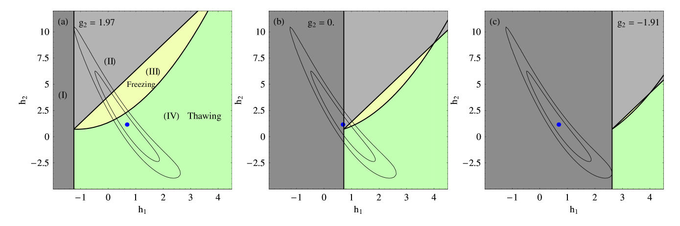
Figure 1: The $h_{1}-h_{2}$ sectors of EXQ: Sector I is the forbidden sector where the scalar field becomes imaginary. Sector II is also forbidden and corresponds to a scalar field that rolls up its potential. Sector III corresponds to ‘freezing’ EXQ where the field is decelerating down its potential towards freezing. Sector IV corresponds to ‘thawing’ EXQ where the scalar field is accelerating down its potential. The forbidden sector I shrinks for a Newton’s constant $G$ that decreases with time ($g_{2}>0$) while the ‘freezing sector’ expands (Fig. 1a). The boundaries of the sectors are provided by (21),(22) and (32). The $1\sigma$, $2\sigma$ $\chi^{2}$ contours obtained from the SNLS SnIa dataset for $\Omega_{0{\rm m}}=0.24$ using the CPL parameterization, are also shown.

Such an analysis is currently in progress pitjeva1 but even before the results become available we can use some heuristic arguments to estimate the order of magnitude of the expected constraints on $g_{i}$ ($i\geq 2$) given the current solar system data.

Current solar system gravity experiments are utilizing lunar laser ranging Muller:2005sr and high precision planet ephemerides data pitjeva to compare the trajectories of celestial bodies with those predicted by general relativity. The possible deviation from the general relativity predictions is parameterized Muller:2005sr using the PPN parameters $\beta$ and $\gamma$, the first current derivative of Newton’s constant $\frac{{\dot{G}}_{0}}{G_{0}}$ and a Yukawa coupling correction to Newton’s inverse square law. These experiments have been collecting data for a time $\Delta t$ of several decades Muller:2005sr ; pitjeva ie $\Delta t={\cal O}(100yrs)$. The current $1\sigma$ constraint pitjeva of

$$|\frac{{\dot{G}}_{0}}{G_{0}}|=|-0.2\pm 0.5|\times 10^{-13}yrs^{-1}<10^{-13}yrs^{-1}$$ (23)

implies an upper bound on the total variation $\frac{\Delta G}{G_{0}}$ over the time-scale $\Delta t$ of approximately

$$|\frac{\Delta G}{G_{0}}|\simeq|\frac{{\dot{G}}_{0}}{G_{0}}|\Delta t<10^{-11}$$ (24)

The same bound is obtained by considering the relative error in the orbital periods $T$ of the Earth and other planets which at $1\sigma$ is pitjeva

$$\frac{\Delta T}{T}<10^{-12}$$ (25)

Given that the Keplerian orbital period is

$$T_{K}=\sqrt{\frac{4\pi^{2}r^{3}}{Gm}}\sim G^{-\frac{1}{2}}$$ (26)

we find

$$|\frac{\Delta T}{T}|=\frac{1}{2}|\frac{\Delta G}{G_{0}}|<10^{-12}$$ (27)

in rough agreement with (24).

Using the upper bound (24) and attributing any variation of $G$ to a term quadratic in $\Delta t$ we get

$$|\frac{\Delta G}{G_{0}}|\simeq|\frac{{\ddot{G}}_{0}}{G_{0}}|(\Delta t)^{2}<10^{-11}$$ (28)

which implies that

$$|\frac{{\ddot{G}}_{0}}{G_{0}}|<10^{-15}yrs^{-2}\implies|g_{2}|<10^{5}h^{-2}$$ (29)

giving a rough order of magnitude estimate of the upcoming constraints on $g_{2}$. Preliminary results from the analysis of solar system data indicate that privateMuller

$$\frac{{\ddot{G}}_{0}}{G_{0}}\simeq(4\pm 5)\cdot 10^{-15}yrs^{-2}$$ (30)

which is not far off the rough estimate of equation (29). Generalizing the above arguments to arbitrary order in $\Delta t$ we find

$$|g_{n}|<10^{8n-11}h^{-n}$$ (31)

which implies that current solar system tests can not constrain $g_{n}$ in any cosmologically useful way for $n\geq 2$.

We now return to the constraint equations (21) and (22) and supplement them by the constraint obtained from the inequality (9). Using the expansions (12), (13) and (14) in equation (7) and equating terms of first order in $z$ we find

$$U_{1}=U^{\prime}(z=0)=\frac{1}{2}(5h_{1}-2h_{2}-9\Omega_{0{\rm m}}+5g_{2}+g_{3})>0$$ (32)

where as usual we have ignored terms proportional to $g_{1}$ due to (20). We now may use (21), (22) and (32) to define the following sectors in the $h_{1}-h_{2}$ parameter space for fixed $g_{1}$, $g_{2}$:

• A forbidden sector I where the inequality (21) is violated.

• A forbidden sector II where the inequality (32) is violated but not the inequality (21).

• An allowed sector III of freezing EXQ where the inequalities (8), (9) and (10) are respected while (11) is violated.

• An allowed sector IV of thawing EXQ where the inequalities (8), (9) and (11) are respected while (10) is violated.

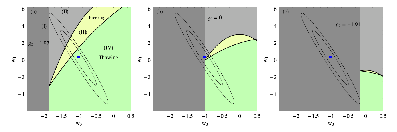
Figure 2: The sectors I-IV of Fig. 1 mapped on the $w_{0}-w_{1}$ parameter space. The allowed sectors extend to $w_{0}<-1$ for $g_{2}>0$.

These sectors are shown in Fig. 1 for $\Omega_{0{\rm m}}=0.24$Spergel:2006hy , $g_{3}=0$ and three values of $g_{2}$: $g_{2}=1.97$, $g_{2}=0$ and $g_{2}=-1.91$.

It would be interesting to superpose on these sectors of Fig. 1 the parameter $\chi^{2}$ contours obtained by fitting to the SnIa data. It is not legitimate however to extrapolate the expansions in powers of $z$ out to $z={\cal O}(1)$ where the SnIa data extend. We thus use an extrapolationChevallier:2000qy ; Linder:2002et with several useful properties first proposed by Chevallier and PolarskiChevallier:2000qy and later investigated in more detail by LinderLinder:2002et . We superpose on the sectors of Fig. 1, the $1\sigma$ and $2\sigma$ $h_{1}-h_{2}$ $\chi^{2}$ contours obtained by fitting the Chevalier-Polarski-Linder (CPL) Chevallier:2000qy ; Linder:2002et parametrization

$$H^{2}(z) = H_{0}^{2}[\Omega_{0m}(1+z)^{3}+$$ (33)

$$+ (1-\Omega_{0m})(1+z)^{3(1+w_{0}+w_{1})}e^{\frac{-3w_{1}z}{(1+z)}}]$$

to the SNLS dataset Astier:2005qq with the same $\Omega_{0{\rm m}}$ prior ($\Omega_{0{\rm m}}=0.24$). Using equation (33) along with the expansion (13) it is easy to show that

$$h_{1} = 3(1+w_{0}-\Omega_{0{\rm m}}w_{0})$$ (34)

$$h_{2} = \frac{3}{2}(2+5w_{0}(1-\Omega_{0{\rm m}})+$$ (35)

$$+ (1-\Omega_{0{\rm m}})(3w_{0}^{2}+w_{1}))$$

so that the standard $\chi^{2}$ contours in the $w_{0}-w_{1}$ space (see eg Nesseris:2005ur ) can be easily translated to the $h_{1}-h_{2}$ space of Fig. 1. The CPL parametrization (33) is constructed so that the parameter $w(z)$ defined as

$$w(z)=\frac{\frac{2}{3}(1+z)\frac{dlnH}{dz}-1}{1-\frac{H_{0}^{2}}{H^{2}}\Omega_{0{\rm m}}(1+z)^{3}}$$ (36)

to be of the form

$$w(z)=w_{0}+w_{1}\frac{z}{1+z}$$ (37)

which has useful and physically motivated propertiesLinder:2002et . The parameter $w(z)$ is particularly useful and physically relevant in the MCQ limit of $g_{i}\rightarrow 0$. In that limit $w(z)$ becomes the MCQ equation of state parameter ie

$$w(z)=\frac{p_{MCQ}}{\rho_{MCQ}}=\frac{\frac{1}{2}{\dot{\Phi}}^{2}-U(\Phi)}{\frac{1}{2}{\dot{\Phi}}^{2}+U(\Phi)}$$ (38)

as may be shown from the MCQ Friedman equations. The values of $g_{2}$ used in Figs 1a and 1c were motivated by demanding minimum and maximum overlap of the forbidden sector I with the $2\sigma$ $h_{1}-h_{2}$ contour.

The following comments can be made with respect to Fig. 1:

• For values of $g_{2}<-1.91$, the $2\sigma$ parameter contour obtained from SNLS lie entirely in the forbidden sector. This bound is independent of $g_{3}$ which does not enter in the inequality (21). Thus in the context of EXQ the constraint on $g_{2}$ obtained by the SNLS data at $2\sigma$ level is

  $$g_{2}=\frac{{\ddot{G}}_{0}}{G_{0}H_{0}^{2}}>-1.91$$ (39)

  Notice the dramatic improvement of this constraint (with respect to the lower bound) compared to the anticipated constraint of $-10^{5}<g_{2}<10^{5}$ anticipated from solar system data (equation (29))!

• The parameter sector III of freezing quintessence is significantly smaller than sector IV of thawing quintessence and the difference is more prominent for smaller $g_{2}$.

• For $g_{2}>0$ the allowed parameter space increases significantly compared to MCQ ($g_{2}=0$). Therefore, if future cosmological observations show preference to the forbidden sectors I or II of Fig. 1b (MCQ) this could be interpreted as evidence for EXQ with $g_{2}>0$ (see also comments in Refs. Perivolaropoulos:2005yv ; Nesseris:2006er ; Gannouji:2006jm )

Even though the plots of Fig. 1 capture the full physical content of our results it is useful to express the sectors I-IV in terms of parameter pairs other than $h_{1}-h_{2}$ which are more common in the literature. Such parameters are the expansion coefficients $w_{i}$ of $w(z)$

$$w(z)=w_{0}+w_{1}z+w_{2}z^{2}+...$$ (40)

which is connected to $H(z)$ via equation (36). By expanding both sides of equation (36) using equations (13) and (40) we may express $h_{i}$ in terms of $w_{i}$ thus rederiving equations (34) and (35) for $i=0$ and $i=1$. The result is identical since the $w_{0}$, $w_{1}$ expansion coefficients of equation (40) coincide with the $w_{0}$, $w_{1}$ coefficients of the CPL parametrization for a $w(z)$ given by equation (37). The advantage of using the parameters $w_{0}-w_{1}$ instead of $h_{1}-h_{2}$ is that they provide better contact with previous studies and can illustrate clearly the fact that a $g_{2}>0$ can provide a phantom behavior $w_{0}<-1$ and crossing of the phantom divide line $w=-1$ in EXQ models.

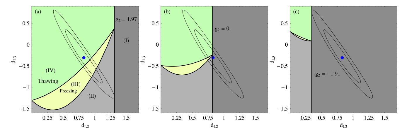
Figure 3: The sectors I-IV of Fig. 1 mapped on the $d_{L2}-d_{L3}$ parameter space. Notice that in this case the forbidden sector I is on the right (large $d_{L2}$).

Using equations (34) and (35) we may express the constraint equations (21), (22) and (32) that define the sectors I-IV in Fig. 1 in terms of $w_{0}-w_{1}$. The resulting equations are

$$3(1-\Omega_{0{\rm m}})(1+w_{0})+g_{2}=\Phi_{1}^{2}>0$$ (41)

$$3(1-\Omega_{0{\rm m}})((1+w_{0})(3\Omega_{0{\rm m}}w_{0}-2)+w_{1})-$$

$$-g_{2}(4+3(1-\Omega_{0{\rm m}})w_{0})-g_{3}=(\Phi^{{}^{\prime}2})^{\prime}(z=0)$$ (42)

$$\frac{3}{2}(1-\Omega_{0{\rm m}})(3(1-w_{0}^{2})-w_{1})+\frac{5}{2}g_{2}+\frac{g_{3}}{2}>0$$ (43)

In the MCQ limit ($g_{2}\rightarrow 0$, $g_{3}\rightarrow 0$) equation (43) has also been obtained in Ref. Scherrer:2005je as a generic limit of MCQ. Using now (41)-(43) along with the $w_{0}-w_{1}$ $\chi^{2}$ contours obtained from the SNLS dataset Astier:2005qq ; Nesseris:2005ur we construct Fig. 2 which is a mapping of Fig. 1 on the $w_{0}-w_{1}$ parameter space. An interesting point of Fig. 2 is that for $g_{2}>0$ (Fig. 2a) the forbidden sector I shrinks significantly compared to MCQ (Fig. 2b) and allows for a $w_{0}<-1$.

A final set of parameters we consider is the set of the expansion coefficients of the luminosity distance $d_{L}(z)$ which in a flat universe is connected to the Hubble expansion history $H(z)$ as

$$H(z)^{-1}=\frac{d}{dz}\left(\frac{d_{L}(z)}{1+z}\right)$$ (44)

Expanding $d_{L}(z)$ as

$$d_{L}(z)=z+d_{L2}z^{2}+d_{L3}z^{3}+...$$ (45)

and using the expansion (13) in equation (44) we may express the coefficients $h_{1}-h_{2}$ in terms of $d_{L2}-d_{L3}$ as follows

$$h_{1} = 4(1-d_{L2})$$ (46)

$$h_{2} = 6(1-3d_{L2}+2d_{L2}^{2}-d_{L3})$$ (47)

Substituting now equations (46), (47) in equations (21), (22) and (32) we obtain the sector equations in $d_{L2}-d_{L3}$ space as

$$4(1-d_{L2})-3\Omega_{0{\rm m}}+g_{2}=\Phi_{1}^{2}>0$$ (48)

$$4d_{L2}(2d_{L2}+g_{2}-3\Omega_{0{\rm m}})+9\Omega_{0{\rm m}}-$$

$$-8-12d_{L3}-5g_{2}-g_{3}=(\Phi^{{}^{\prime}2})^{\prime}(z=0)$$ (49)

$$4+8d_{L2}-12d_{L2}^{2}+6d_{L3}-\frac{9}{2}\Omega_{0{\rm m}}+$$

$$+\frac{5}{2}g_{2}+\frac{g_{3}}{2}>0$$ (50)

Using now equations (46), (47) to translate the $h_{1}-h_{2}$ $\chi^{2}$ contours to the $d_{L2}-d_{L3}$ parameter space and equations (48)-(50) to construct the sectors I-IV in the $d_{L2}-d_{L3}$ space we obtain Fig. 3. The advantage of Fig. 3 compared to Figs. 1 and 2 is that it refers to the parameters $d_{L2}-d_{L3}$ which are directly observable through the luminosity distances of SnIa without the need of any differentiation.

III Conclusion-Discussion-Outlook

We have used generic theoretically motivated inequalities to investigate the space of observable cosmological expansion parameters that admits viable MCQ and EXQ theoretical models. Our inequalities are generic in the sense that they are independent of the specific features of any scalar field potential (eg scale, tracking behavior etc) and they only require that the models are internally consistent. The derived forbidden sectors which violate the above inequalities already have significant overlap with the parameter space which is consistent with observations at the $2\sigma$ level. This overlap which depends on the time derivatives of the Newton’s constant $G$ has lead to a useful constraint to the second derivative of $G$ (equation (39)) which is significantly more stringent compared to the corresponding constraint (29) anticipated from solar system gravity experiments .

An important reason that limits the observable parameter space consistent with MCQ and EXQ is the fact that the scalar field potential energy can induce accelerating expansion but not beyond the limit corresponding to the cosmological constant ($w(z)=-1$) obtained when the field’s evolution is frozen. Additional acceleration (superacceleration) can only be provided in the context of EXQ through the time variation of Newton’s constant $G$. A decreasing $G(t)$ with time favors accelerating expansion and allows for superacceleration. This physical argument is reflected in our results. We found that given ${\dot{G}}_{0}\simeq 0$ (neglecting $g_{1}$ since $|g_{1}|<10^{-4}$ from solar system tests) a ${\ddot{G}}_{0}>0$ ($g_{2}>0$) decreases the forbidden sector and allows superacceleration ($w_{0}<-1$). But ${\dot{G}}_{0}\simeq 0$ with ${\ddot{G}}_{0}>0$ implies that we are currently close to a minimum of $G(t)$ with $G(t)$ being larger in the past ie

$$\frac{G(t)}{G_{0}}\simeq 1+\frac{1}{2}g_{2}(H_{0}(t-t_{0}))^{2}$$ (51)

Therefore a decreasing $G(t)$ corresponds to ${\ddot{G}}_{0}>0$ ($g_{2}>0$) (see Fig. 4) which in turn implies smaller forbidden sectors and allows for superacceleration in agreement with the above physical argument.

Figure 4: A $g_{2}>0$ implies a decreasing Newton’s constant ($\frac{G(t)}{G_{0}}\simeq 1+\frac{1}{2}g_{2}(H_{0}(t-t_{0}))^{2}$ around $t=t_{0}$).

An additional interesting point is related to the construction of the $\chi^{2}$ contours of Figs. 1-3. The SNLS data analysis involved in the construction of these contours did not take into account the possible evolution of SnIa due to the evolving $G(t)$. It is straightforward to take into account the evolution of $G$ in the SnIa data analysis along the lines of Ref. Nesseris:2006jc . In order to test the sensitivity of these contours with respect to the evolution of $G$ we have repeated the $\chi^{2}$ contour construction assuming a varying $G$ according to the ansatz

$$G(z)=G_{0}(1+\alpha\frac{z^{2}}{(1+z)^{2}})$$ (52)

which smoothly interpolates between the present value of $G=G_{0}$ and the high redshift value $G=G_{0}(1+\alpha)$ implying that

$$\alpha=\frac{\Delta G}{G_{0}}$$ (53)

The parametrization (52) is consistent with both the solar system testspitjeva ($\frac{{\dot{G}}_{0}}{G_{0}}\simeq 0$) and the nucleosynthesis constraintsCopi:2003xd

$$|\frac{G_{nuc}-G_{0}}{G_{0}}|<0.2$$ (54)

at $1\sigma$, for $|\alpha|<0.2$.

It is straightforward to evaluate $g_{1},g_{2},g_{3}$ in terms of $\alpha$ using the parametrization (52) and equation (16). The result is

$$g_{1}=0$$ (55)

$$g_{2}=2\alpha$$ (56)

$$g_{3}=3\alpha\left(-1+3w_{0}(-1+\Omega_{0{\rm m}})\right)$$ (57)

We have considered the value of

$$\alpha=0.2$$ (58)

and repeated the SNLS data analysis taking into account the evolution of the SnIa absolute magnitude $M$ due to the evolving $G$ Bond:1984sn ; Colgate:1966ax ; Amendola:1999vu ; Nesseris:2006jc as

$$M=M_{0}+\frac{15}{4}log\frac{G}{G_{0}}$$ (59)

The steps involved in this analysis may be summarized as follows:

• Use the following magnitude redshift relation to fit to the SnIa data

  $$m_{th}(z)=M_{0}+5logd_{L}(z)+\frac{15}{4}log\frac{G(z)}{G_{0}}$$ (60)

  where $G(z)$ is given by (52) and $d_{L}(z)$ is connected to $H(z)$ in the usual geometrically defined way (44) ie

  $$d_{L}(z)=(1+z)\int_{0}^{z}dz^{\prime}\frac{1}{H(z^{\prime})}$$ (61)

• Use an $H(z)$ parametrization that incorporates the evolution of $G$ (given by (52)) in the context of the CPL parametrization (33) ie

  $$H^{2}(z) = \frac{G(z)}{G_{0}}H_{0}^{2}[\Omega_{0m}(1+z)^{3}+$$ (62)

  $$+ (1-\Omega_{0m})(1+z)^{3(1+w_{0}+w_{1})}e^{\frac{-3w_{1}z}{(1+z)}}]$$

• Minimize the $\chi^{2}$ expression

  $$\chi^{2}(w_{0},w_{1})=\sum_{i}\frac{(m^{obs}(z_{i})-m^{th}(z_{i};w_{0},w_{1}))^{2}}{\sigma_{m^{obs}(z_{i})}^{2}}$$ (63)

  and find the corresponding $1\sigma$ and $2\sigma$ $\chi^{2}$ contours along the lines of Refs. Nesseris:2005ur ; Nesseris:2006jc

The resulting $\chi^{2}$ contours in the $w_{0}-w_{1}$ space are shown in Fig. 5 (dashed lines) superposed with the corresponding contours constructed by neglecting the evolution of $G$ (continuous lines).

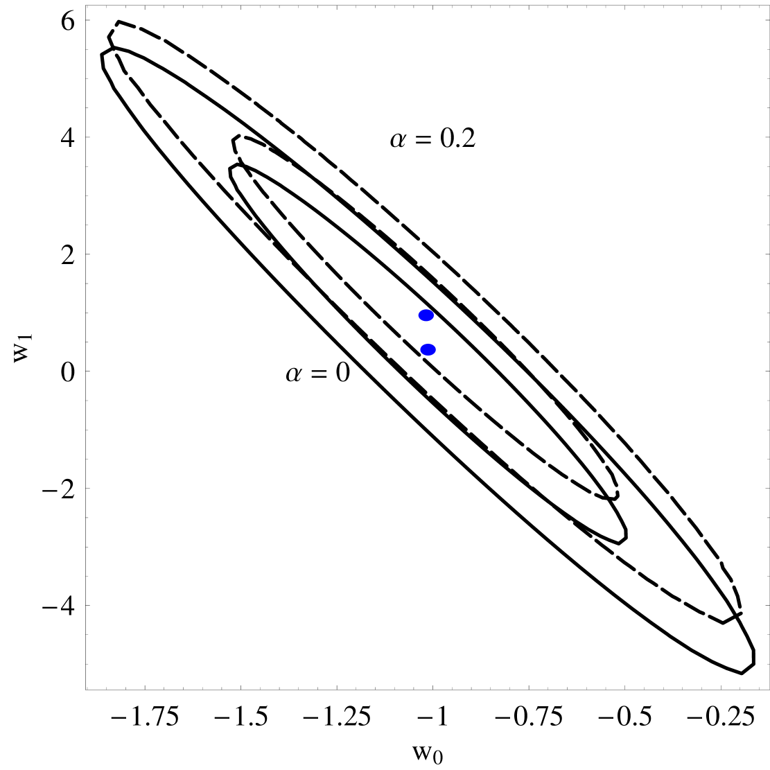
Figure 5: Taking into account a $G$ variation consistent with the nucleosynthesis and solar system bounds introduces modifications to the $w_{0}-w_{1}$ $\chi^{2}$ contours which are not significant for the currently available SnIa data (for the dashed line $\alpha=0.2$ and the continuous $\alpha=0$).

The change of the best fit $w_{0}-w_{1}$ values and of the corresponding errorbars is minor (especially in the $w_{0}$ direction) and such that our main conclusion regarding the limiting values of $g_{2}$ remain practically unchanged even after the evolution of $G$ is taken into account in the analysis. This justifies neglecting the evolution of $G$ in the construction of the $\chi^{2}$ contours for our purposes. However, as the quality of SnIa data improves, it becomes clear from Fig. 5 that the effects of an evolving $G$ consistent with nucleosynthesis and solar system constraints on the data analysis can be significant! This possibility is further amplified if there are additional effects of an evolving $G$ on the SnIa data analysis. For example linder-www ; smchdep it is possible that the time scale stretch factor $s$ involved in the SnIa data analysis Astier:2005qq ; Nesseris:2005ur and arising from opacity effects in the stellar atmosphere may have a dependence on the Chandrasekhar mass and therefore on Newton’s constant $G$. We have shown however that even if such effects are included in the SnIa data analysis our results of Fig. 5 (dashed line) do not change more than $10\%$.

An interesting extension of the present work could involve the investigation of the limits of other dark energy models like braneworld models or barotropic fluid dark energy in the context of scalar-tensor theories (thus extending the results of Scherrer Scherrer:2005je ). The identification of the forbidden observational parameter regions for such models could be combined with the constraints of local gravitational experiments to test the internal consistency of these models. Alternatively the present work could be extended in the direction of finding the limits and cosmological consistency of specific classes of potentials in the context of EXQ thus also extending the work of Sahlen:2006dn ; Huterer:2006mv ; Li:2006ea .

Numerical Analysis: Our numerical analysis was performed using a Mathematica code available at http://leandros.physics.uoi.gr/exqlim/exqlim.htm

References

- (1) P. Astier et al., Astron. Astrophys. 447, 31 (2006) [arXiv:astro-ph/0510447].
- (2) A. G. Riess et al. [Supernova Search Team Collaboration], Astrophys. J. 607, 665 (2004) [arXiv:astro-ph/0402512].
- (3) Riess A et al., 1998 Astron. J. 116 1009; Perlmutter S J et al., 1999 Astroph. J. 517 565; Tonry, J L et al., 2003 Astroph. J. 594 1; Barris, B et al., 2004 Astroph. J. 602 571; Knop R et al., 2003 Astroph. J. 598 102;
- (4) S. W. Allen, R. W. Schmidt, H. Ebeling, A. C. Fabian and L. van Speybroeck, Mon. Not. Roy. Astron. Soc. 353, 457 (2004) [arXiv:astro-ph/0405340].
- (5) D. J. Eisenstein et al. [SDSS Collaboration], Astrophys. J. 633, 560 (2005) [arXiv:astro-ph/0501171].
- (6) D. N. Spergel et al., arXiv:astro-ph/0603449.
- (7) E. J. Copeland, M. Sami and S. Tsujikawa, arXiv:hep-th/0603057.
- (8) T. Padmanabhan, arXiv:astro-ph/0603114.
- (9) L. Perivolaropoulos, arXiv:astro-ph/0601014.
- (10) V. Sahni and A. Starobinsky, arXiv:astro-ph/0610026.
- (11) S. M. Carroll, Living Rev. Rel. 4, 1 (2001) [arXiv:astro-ph/0004075].
- (12) V. Sahni and A. A. Starobinsky, Int. J. Mod. Phys. D 9, 373 (2000) [arXiv:astro-ph/9904398].
- (13) B. Ratra and P. J. E. Peebles, Phys. Rev. D 37, 3406 (1988).
- (14) R. R. Caldwell, R. Dave and P. J. Steinhardt, Phys. Rev. Lett. 80, 1582 (1998) [arXiv:astro-ph/9708069].
- (15) I. Zlatev, L. M. Wang and P. J. Steinhardt, Phys. Rev. Lett. 82, 896 (1999) [arXiv:astro-ph/9807002].
- (16) B. Boisseau, G. Esposito-Farese, D. Polarski and A. A. Starobinsky, Phys. Rev. Lett. 85, 2236 (2000) [arXiv:gr-qc/0001066].
- (17) L. Perivolaropoulos, JCAP 0510, 001 (2005) [arXiv:astro-ph/0504582].
- (18) V. Sahni and Y. Shtanov, JCAP 0311, 014 (2003) [arXiv:astro-ph/0202346].
- (19) C. Bogdanos and K. Tamvakis, arXiv:hep-th/0609100.
- (20) G. Kofinas, G. Panotopoulos and T. N. Tomaras, JHEP 0601, 107 (2006) [arXiv:hep-th/0510207].
- (21) G. R. Dvali, G. Gabadadze and M. Porrati, Phys. Lett. B 484, 112 (2000) [arXiv:hep-th/0002190].
- (22) S. Nojiri and S. D. Odintsov, Phys. Rev. D 74, 086005 (2006) [arXiv:hep-th/0608008].
- (23) G. Esposito-Farese and D. Polarski, Phys. Rev. D 63, 063504 (2001) [arXiv:gr-qc/0009034].
- (24) F. Perrotta, C. Baccigalupi and S. Matarrese, Phys. Rev. D 61, 023507 (2000) [arXiv:astro-ph/9906066].
- (25) R. R. Caldwell and E. V. Linder, Phys. Rev. Lett. 95, 141301 (2005) [arXiv:astro-ph/0505494].
- (26) R. J. Scherrer, Phys. Rev. D 73, 043502 (2006) [arXiv:astro-ph/0509890].
- (27) T. Chiba, Phys. Rev. D 73, 063501 (2006) [arXiv:astro-ph/0510598].
- (28) P.D. Scharre, C.M. Will, Phys. Rev. D 65 (2002); E. Poisson, C.M. Will, Phys. Rev. D 52, 848 (1995).
- (29) R. Gannouji, D. Polarski, A. Ranquet and A. A. Starobinsky, JCAP 0609, 016 (2006) [arXiv:astro-ph/0606287].
- (30) E.V. Pitjeva, Astron. Lett. 31, 340 (2005); Sol. Sys. Res. 39, 176 (2005).
- (31) J. Muller, J. G. Williams and S. G. Turyshev, arXiv:gr-qc/0509114.
- (32) E.V. Pitjeva and J. Muller, private communication.
- (33) J. Muller, private communication.
- (34) M. Chevallier and D. Polarski, Int. J. Mod. Phys. D 10, 213 (2001) [arXiv:gr-qc/0009008].
- (35) E. V. Linder, Phys. Rev. Lett. 90, 091301 (2003) [arXiv:astro-ph/0208512].
- (36) S. Nesseris and L. Perivolaropoulos, Phys. Rev. D 72, 123519 (2005) [arXiv:astro-ph/0511040].
- (37) S. Nesseris and L. Perivolaropoulos, arXiv:astro-ph/0610092.
- (38) S. Nesseris and L. Perivolaropoulos, Phys. Rev. D 73, 103511 (2006) [arXiv:astro-ph/0602053].
- (39) C. J. Copi, A. N. Davis and L. M. Krauss, Phys. Rev. Lett. 92, 171301 (2004) [arXiv:astro-ph/0311334].
- (40) L. Amendola, P. S. Corasaniti and F. Occhionero, arXiv:astro-ph/9907222; E. Garcia-Berro, E. Gaztanaga, J. Isern, O. Benvenuto and L. Althaus, arXiv:astro-ph/9907440; E. Gaztanaga, E. Garcia-Berro, J. Isern, E. Bravo and I. Dominguez, Phys. Rev. D 65, 023506 (2002) [arXiv:astro-ph/0109299].
- (41) J. R. Bond, W. D. Arnett and B. J. Carr, Astrophys. J. 280, 825 (1984).
- (42) S. A. Colgate and R. H. White, Astrophys. J. 143, 626 (1966).
- (43) E. Linder, private communication, http://supernova.lbl.gov/ evlinder/gdotsn.pdf.
- (44) A. Khokhlov, E. Muller and P. Hoflich, Astron. Astrophys. 270, 223 (1993).
- (45) P. Caresia, S. Matarrese and L. Moscardini, Astrophys. J. 605, 21 (2004) [arXiv:astro-ph/0308147].
- (46) M. Sahlen, A. R. Liddle and D. Parkinson, arXiv:astro-ph/0610812.
- (47) D. Huterer and H. V. Peiris, arXiv:astro-ph/0610427.
- (48) C. Li, D. E. Holz and A. Cooray, arXiv:astro-ph/0611093.