The Low-Mass X-ray Binary and Globular Cluster Connection in Virgo Cluster Early-type Galaxies: Optical Properties

Abstract

Low-mass X-ray binaries (LMXBs) form efficiently in globular clusters (GCs). By combining Chandra X-ray Observatory and Hubble Space Telescope-Advanced Camera for Surveys observations of early-type galaxies, we probe the LMXB-GC connection using the most accurate identification of LMXBs and GCs to date. We explore the optical properties of 270 GCs with LMXBs and 6,488 GCs without detectable X-ray emission from a sample of eleven massive early-type galaxies in the Virgo cluster. Globular clusters that are more massive, are redder, and have smaller radii are more likely to contain LMXBs. Using known structural scaling relations for GCs, the latter implies that denser GCs are more likely to hold LMXBs. Unlike Galactic GCs, a large number of GCs with LMXBs have half-mass relaxation times $>2.5{\rm\,Gyr}$; GCs do not need to survive for more than five relaxation timescales to produce LMXBs. By fitting the dependence of the expected number of LMXBs per GC, $\lambda_{t}$, on the GC mass ${M}$, color $(g-z)$, and half-mass radius $r_{h,{\rm cor}}$, we find that $\lambda_{t}\propto{M}^{1.24\pm 0.08}\,10^{0.9^{+0.2}_{-0.1}\,(g-z)}\,r_{h,{\rm cor}}^{-2.2\pm 0.2}$. This rules out that the number of LMXBs per GC is linearly proportional to GC mass (99.89% confidence limit). We derive an expression to estimate the number of multiple LMXB sources in GCs and predict that most GCs with high X-ray luminosities contain a single LMXB. The detailed dependence of $\lambda_{t}$ on GC properties appears mainly due to a dependence on a combination of mass and radius, and a dependence on color, that are essentially equivalent to a dependence on the encounter rate $\Gamma_{h}$ and the metallicity ${Z}$, $\lambda_{t}\propto\Gamma_{h}^{0.82\pm 0.05}\,{Z}^{0.39\pm 0.07}$. Our analysis provides strong evidence that dynamical formation and metallicity play the primary roles in determining the presence of an LMXB in extragalactic GCs. The shallower than linear dependence of GC sources requires an explanation by theories of dynamical binary formation; however, we note that our use of $\Gamma_{h}$ as a proxy for the encounter rate, particularly if core-collapsed extragalactic GCs preferentially contain LMXBs, needs further testing in nearer galaxies. A metallicity-dependent variation in the number of neutron stars and black holes per unit GC mass, effects from irradiation induced winds, or suppression of magnetic braking in metal-poor stars may all be consistent with our derived abundance dependence; all three scenarios require further development.

1. Introduction

A low-mass X-ray binary (LMXB) consists of a compact stellar remnant, a neutron star (NS) or black hole (BH), that accretes the stellar envelope of a low-mass (${M}\lesssim 2{M}_{\odot}$) stellar companion. Roche-lobe overflow is the major method of mass transfer in these systems, which in the Milky Way have orbital periods of $0.19$–$398{\rm\,hr}$ (White et al. 1995). When actively accreting, LMXBs are bright X-ray sources ($\sim 10^{35}$–$10^{39}{\rm\,erg\,s}^{-1}$; hereafter, the use of “LMXBs” refers only to active LMXBs). The Milky Way ($L_{*}\sim 10^{10}\,L_{\odot}$) contains $\approx 150$ active LMXBs (Liu et al. 2001). Most of these LMXBs are in the field of the Milky Way and are likely to have been the result of the stellar evolution of a primordial binary (Verbunt & van den Heuvel 1995). This primordial formation of an LMXB cannot be particularly efficient as the binary must survive the supernova that forms the NS/BH, yet remain in a tight enough orbit that Roche-lobe overflow eventually occurs.

On the other hand, gravitational interactions in dense stellar systems, particularly globular clusters (GCs), could lead to more efficient formation of binaries in general, and LMXBs in particular. Over the history of X-ray astronomy, 13 active Galactic LMXBs have been detected in 12 GCs (Liu et al. 2001; White & Angelini 2001). In addition to active LMXBs, Galactic GCs may contain seven times as many LMXBs in quiescence (Heinke et al. 2003). Since GCs account for $\sim 0.1\%$ of the Galactic light, but $\sim 10\%$ of the active Galactic LMXBs, formation of LMXBs in GCs must be hundreds of times more efficient than in the field (e.g., Clark 1975; Katz 1975). The increased efficiency may be due to a combination of two effects: (1) LMXB formation through tidal capture or exchange interactions after the supernova of the NS/BH; and (2) tighter binary orbits (binary hardening) in GCs due to exchange interactions. The optical properties of GCs containing LMXBs provide a platform to test the dynamical formation of LMXBs in GCs. Furthermore, the metallicities of GCs can be readily estimated through their optical color, allowing one to probe for metallicity dependence in the evolution or formation processes of LMXBs in GCs. Although some patterns can be seen in the limited Galactic data (e.g., Bellazzini et al. 1995; Bregman et al. 2006, hereafter B06), a larger sample is necessary to probe LMXB formation and evolution in GCs.

With the launch of the Chandra X-ray Observatory (CXO), it is now possible to examine large samples of LMXBs. In particular, X-ray observations of nearby early-type galaxies can identify tens to hundreds of bright X-ray sources, most of which are likely to be LMXBs (e.g., Sarazin et al. 2000). In these galaxies, $\sim 20\%$–$70\%$ of the LMXBs appear to be associated with GCs (e.g., Sarazin et al. 2000, 2001; Angelini et al. 2001; Kundu et al. 2002; Jordán et al. 2004b); early-type galaxies can provide the large number of GCs containing LMXBs necessary to probe LMXB formation and evolution in GCs. Early samples have shown that brighter and redder GCs are more likely to contain LMXBs (e.g. Kundu et al. 2003; Sarazin et al. 2003; Jordán et al. 2004b); however, the use of resolution limited ground-based data or field-of-view (FOV) limited space-based data suppressed the numbers of GCs that could clearly be identified.

By observing nearby early-type galaxies with the Wide Field Channel of the Hubble Space Telescope Advanced Camera for Surveys (HST-ACS/WFC), which has a $3\farcm 2\times 3\farcm 2$ FOV and can resolve GCs in nearby galaxies, one can construct accurate and comprehensive lists of GCs. In particular, the measurement of GC size allows better discrimination against unresolved background sources with GC colors, while providing a GC property that is crucially important for probing the structure of GCs that contain LMXBs. The ACS Virgo Cluster Survey (ACSVCS) has observed the centers of 100 early-type galaxies (Côté et al. 2004) and provides excellent GC data. Some of its initial work explored the GC-LMXB connection in NGC 4486 M87, Jordán et al. 2004b, hereafter ACSVCS3. In this work, we expand upon this analysis exploring the GC-LMXB connection in 10 ACSVCS galaxies and a more nearby galaxy (NGC 4697) that may not belong to Virgo, but was observed following the ACSVCS observational setup. We identify 270 GCs that contain LMXBs; this is one of the largest such samples to date, and the largest sample that includes information about GC size.

Table 1Galaxy Properties of Sample

	Type	$r_{\rm eff}$	$D_{\rm SBF}$	$M_{B}$
Galaxy	(RC3)	(arcsec)	(Mpc)	(mag)	Other Names
(1)	(2)	(3)	(4)	(5)
NGC 4365 (catalog )	E3	049.8	23.2	-21.46	VCC731
NGC 4374 (catalog )	E1	051.0	18.7	-21.45	M84, VCC763
NGC 4382 (catalog )	S0	054.6	17.9	-21.46	M85, VCC798
NGC 4406 (catalog )	E3	104.0	18.0	-21.56	M86, VCC881
NGC 4472 (catalog )	E2	104.0	16.8	-21.98	M49, VCC1226
NGC 4486 (catalog )	E0	094.9	15.7	-21.70	M87, VCC1316
NGC 4526 (catalog )	S0	044.4	16.1	-20.60	VCC1535
NGC 4552 (catalog )	E0	029.3	16.1	-20.55	M89, VCC1632
NGC 4621 (catalog )	E5	040.5	15.0	-20.37	M59, VCC1903
NGC 4649 (catalog )	E2	068.7	16.4	-21.39	M60, VCC1978
NGC 4697 (catalog )	E6	072.0	11.3	-20.29

2. Sample

2.1. Galaxy Sample

We selected our sample from early-type Virgo galaxies with detections of LMXBs using CXO and GCs using HST-ACS. Since the most massive galaxies are the most likely to have large populations of both LMXBs and GCs, we concentrated on galaxies with $M_{B}<-20.25$. Our sample includes the ten brightest ACSVCS galaxies (NGC 4472, 4486, 4406, 4365, 4382, 4374, 4649, 4526, 4552, and 4621) and NGC 4697, a similarly bright galaxy, which we observed with nearly the same setup as the ACSVCS. Table 1 summarizes some properties of the galaxies in our sample. The first three columns list the name, Hubble type, and effective radius $r_{\rm eff}$ from de Vaucouleurs et al. (1992). The next columns list the (polynomial calibrated) surface brightness fluctuation distance, $D_{\rm SBF}$, determined from the HST observations (Mei et al. 2006) and the absolute total B-magnitude, $M_{B}$ (combining $b_{t}$ from HyperLeda and $D_{\rm SBF}$).

2.2. X-ray Analysis

Table 2Properties of Chandra Observations

			$t_{\rm obs}$	$t_{\rm exp}$
Galaxy	OBSID	Detector	(ks)	(ks)
(1)	(2)	(3)	(4)	(5)
NGC 4365	2015 (catalog ADS/Sa.CXO#obs/02015)	ACIS-S3/F	40.4	40.4
NGC 4374	0803 (catalog ADS/Sa.CXO#obs/00803)	ACIS-S3/VF	28.5	28.4
NGC 4382	2016 (catalog ADS/Sa.CXO#obs/02016)	ACIS-S3/F	39.7	39.7
NGC 4406	0318 (catalog ADS/Sa.CXO#obs/00318)	ACIS-S3/F	14.6	11.4
$\cdots$	0963 (catalog ADS/Sa.CXO#obs/00963)	ACIS-S3/F	14.8	12.0
NGC 4472	0321 (catalog ADS/Sa.CXO#obs/00321)	ACIS-S3/VF	39.6	34.5
$\cdots$	0322 (catalog ADS/Sa.CXO#obs/00322)	ACIS-I/VF	10.4	07.2
NGC 4486	0352 (catalog ADS/Sa.CXO#obs/00352)	ACIS-S3/G	37.7	33.6
$\cdots$	2707 (catalog ADS/Sa.CXO#obs/02707)	ACIS-S3/F	98.7	82.2
$\cdots$	3717 (catalog ADS/Sa.CXO#obs/03717)	ACIS-S3/F	20.6	09.2
NGC 4526	3925 (catalog ADS/Sa.CXO#obs/03925)	ACIS-S3/VF	43.5	41.5
NGC 4552	2072 (catalog ADS/Sa.CXO#obs/02072)	ACIS-S3/VF	54.4	54.4
NGC 4621	2068 (catalog ADS/Sa.CXO#obs/02068)	ACIS-S3/F	24.8	24.8
NGC 4649	0785 (catalog ADS/Sa.CXO#obs/00785)	ACIS-S3/VF	36.9	17.0
NGC 4697	0784 (catalog ADS/Sa.CXO#obs/00784)	ACIS-S3/F	39.3	37.2
$\cdots$	4727 (catalog ADS/Sa.CXO#obs/04727)	ACIS-S3/VF	39.9	39.9
$\cdots$	4727 (catalog ADS/Sa.CXO#obs/04727)	ACIS-S3/VF	35.6	35.6
$\cdots$	4729 (catalog ADS/Sa.CXO#obs/04729)	ACIS-S3/VF	38.1	32.0
$\cdots$	4730 (catalog ADS/Sa.CXO#obs/04730)	ACIS-S3/VF	40.0	40.0

These galaxies all had archival or proprietary data from CXO; however, the observational setup varied widely between galaxies. Table 2 summarizes the properties of the CXO observations, listing the galaxy name, CXO observation number (OBSID), detector with data mode (Faint, Graded, or Very-Faint), and the exposure times before ($t_{\rm obs}$) and after removing periods of high backgrounds ($t_{\rm exp}$). Since the ACIS-I chips are less sensitive than the ACIS-S3 chip, we only include data from ACIS-I when its $t_{\rm obs}$ is $>25\%$ the $t_{\rm obs}$ of the ACIS-S3. Since the HST-ACS FOV is smaller than the CXO FOV, we hereafter only discuss X-ray sources within the CXO/HST overlapping region.

All CXO observations were analyzed under ciao 3.1 with caldb 2.28 and NASA’s FTOOLS 5.3. For Observation 0784, the focal plane temperature was $-110^{\circ}$ C, while all other observations were taken at $-120^{\circ}$ C. When Very-Faint mode telemetry was available, the observations were cleaned using the extra data available in this mode to reduce the background level. All other observations were reduced in Faint mode, including OBSID 0352, which was telemetered in “Graded” mode. Known aspect offsets were applied for each observation. Our analysis includes only events with ASCA grades of 0, 2, 3, 4, and 6. Photon energies were determined using the gain files acisD2000-01-29gain_ctiN0001.fits, except for OBSIDs 0352 (acisD2000-07-06gainN0003.fits) and 0784 (acisD1999-09-16gainN0005.fits). When appropriate, we corrected for time dependence of the gain and the charge-transfer inefficiency. All observations were corrected for quantum efficiency (QE) degradation and had exposure maps determined at $750{\rm\,eV}$. We excluded bad pixels, bad columns, and columns adjacent to bad columns or chip node boundaries.

The use of local backgrounds in point source analysis mitigates the effect of high background periods (“background flares”), which especially affect the backside-illuminated S1 and S3 chips. We avoided the periods with the most extreme flares by only including times where the background rate was below three times the expected rate from the blank-sky background fields in the CALDB. When available, we used the S1 chip to measure the background rate, excluding point sources, and compared to the blank-sky background count rates in CALDB in the $2.6$–$6.0{\rm\,keV}$ band. If the S1 chip was not available, we used the S3 chip to determine count rates in the $2.6$–$7.0{\rm\,keV}$ band. For Observation 0784, we compared count rates in the 0.3–10.0 keV band to Maxim Markevitch’s aciss_B_7_bg_evt_271103.fits blank-sky background. When we binned the observations regularly in time to determine the count rate, small time intervals at the edges of the existing good-time intervals could not be included in a bin. This led to only a small amount of time that was lost in any observation. We list the exposure before and after flare removal in Table 2.

To identify the discrete X-ray source population, we applied a wavelet detection algorithm (the CIAO wavdetect program) with scales increasing by a factor of $\sqrt{2}$ from 1 to 32 pixels. We adopted a source detection threshold of $10^{-6}$ ($\lesssim 1$ false source per chip) for both the ACIS S3 and I chips. Source detection excluded regions with an exposure of less than 10% of that of the observation (e.g., regions at the edges of chips). To maximize the signal-to-noise (S/N), we analyzed the wavelet detection results from combined observations when available. We detected 708 X-ray sources that were also in the FOV of the HST-ACS observations. There are regions of complex gas emission at the center of NGC 4486. Although detected sources in these region may be LMXBs, they may also be compact regions of enhanced gas emission. To avoid mistaken identification of point sources, ACSVCS3 excluded all X-ray sources in these regions. We follow this procedure, excluding 33 X-ray sources.

We used the coordinate list generated by wavdetect in ACIS Extract 3.34 to refine the source positions and determine source extraction regions. This was accomplished by determining the mean positions of events in source extraction regions consistent with the X-ray point spread functions (PSFs) at the positions of the sources. For most sources the median photon energy was $0.6$–$2.6{\rm\,keV}$ and we required the extraction region to encircle 90% of the X-ray PSF at $1.5{\rm\,keV}$. We determined the PSF at either $0.3{\rm\,keV}$ or $4.5{\rm\,keV}$ for the few sources whose median photon energy was either softer or harder. In a few sources where the 90% PSF extraction regions overlapped, we used a lower percentage of the PSF to define the extraction region.

When there were multiple observations of a galaxy, we matched the positions of detected sources in individual observations to those present in the observation with the largest exposure. Absolute astrometric corrections were applied for all sources in all galaxies using a two-dimensional cross-correlation technique to match sources from the Tycho-2 Catalog (Høg et al. 2000), 2MASS Point Source and Extended Source Catalogs, and the USNO-B Catalog (Monet et al. 2003). An astrometric correction (separately in RA and Dec.) was applied if the offset was statistically significant.

We used a local background from an annular region whose area was approximately three times that of each source’s extraction region; these local backgrounds include the diffuse emission from the host galaxy. To insure that the local background regions did not contain any significant number of source counts, the inner radius of the background region was taken to be the radius encircling 97% of the PSF. In cases where background regions overlapped or fell along node/chip boundaries, we slightly altered these overlapping regions, preserving the ratio of source to background areas and ensuring that the source region and background region had similar mean exposures. For each of the sources, the observed net count rates, their errors, and S/N were calculated in the $0.3$–$6.0{\rm\,keV}$ band by stacking the observations for each galaxy, correcting for background photons, and dividing by the sum of the mean exposure over each source region. In NGC 4374 and NGC 4486, a few of the sources detected with wavdetect had negative net count rates when determined in this way (two sources in NGC 4374, five sources in NGC 4486); we excluded these sources from further discussion.

Table 3GC-LMXB Matches by Galaxies

Galaxy	$N_{X}$	$L_{X,{\rm min}}$	$N_{\rm GCs}$	$(g-z)_{\rm div}$	$N_{\rm Blue\,GCs}$	$N_{\rm Red\,GCs}$	$N_{\rm GCs\,w\,LMXBs}$	$N_{\rm Blue\,GCs\,w\,LMXBs}$	$N_{\rm Red\,GCs\,w\,LMXBs}$	$N_{\rm False\,Matches}$
(1)	(2)	(3)	(4)	(5)	(6)	(7)	(8)	(9)	(10)	(11)
Detected: All Sources With Positive Luminosity
NGC 4365	85	0.10	0906	1.160	418 [3]	488 [7]0	43 (5)	11 (0)	29 (2)	4.36
NGC 4374	49	0.05	0506	1.200	310 [0]	196 [0]0	18 (0)	09 (0)	09 (0)	1.85
NGC 4382	37	0.52	0505	1.230	320 [1]	185 [1]0	11 (1)	07 (0)	03 (0)	1.40
NGC 4406	28	0.09	0367	1.220	260 [0]	107 [0]0	06 (0)	04 (0)	02 (0)	0.75
NGC 4472	86	0.57	0764	1.180	306 [0]	458 [4]0	40 (2)	04 (0)	36 (2)	2.83
NGC 4486	84	0.14	1639	1.190	690 [4]	949 [10]	49 (6)	12 (0)	34 (3)	6.95
NGC 4526	34	0.31	0244	1.170	121 [0]	123 [0]0	07 (0)	03 (0)	04 (0)	0.98
NGC 4552	78	0.15	0455	1.190	217 [1]	238 [1]0	31 (1)	08 (0)	22 (0)	3.00
NGC 4621	44	0.39	0306	1.110	121 [0]	185 [2]0	17 (1)	01 (0)	16 (1)	1.24
NGC 4649	60	0.65	0806	1.200	335 [0]	471 [0]0	32 (0)	03 (0)	29 (0)	1.50
NGC 4697	83	0.06	0298	1.127	127 [2]	171 [2]0	34 (2)	07 (1)	27 (1)	2.15
SNR: All Sources with Luminosities Determined at the 3$\sigma$ Level
NGC 4365	29	2.26	0906	1.160	418 [1]	488 [5]0	17 (3)	01 (0)	15 (2)	1.25
NGC 4374	16	2.18	0506	1.200	310 [0]	196 [0]0	05 (0)	02 (0)	03 (0)	0.62
NGC 4382	21	1.64	0505	1.230	320 [0]	185 [0]0	05 (0)	04 (0)	01 (0)	0.86
NGC 4406	19	2.65	0367	1.220	260 [0]	107 [0]0	06 (0)	04 (0)	02 (0)	0.44
NGC 4472	54	1.30	0764	1.180	306 [0]	458 [2]0	26 (1)	03 (0)	23 (1)	1.72
NGC 4486	61	1.30	1639	1.190	690 [3]	949 [5]0	40 (3)	09 (0)	29 (1)	3.65
NGC 4526	12	1.30	0244	1.170	121 [0]	123 [0]0	03 (0)	01 (0)	02 (0)	0.33
NGC 4552	49	0.80	0456	1.190	217 [1]	239 [1]0	25 (1)	06 (0)	18 (0)	1.53
NGC 4621	16	1.58	0306	1.110	121 [0]	185 [0]0	04 (0)	00 (0)	04 (0)	0.55
NGC 4649	21	2.85	0807	1.200	335 [0]	472 [0]0	13 (0)	02 (0)	11 (0)	0.43
NGC 4697	66	0.15	0298	1.127	127 [2]	171 [2]0	26 (2)	07 (1)	19 (1)	1.75
Complete: All Sources with Luminosities $>3.2\times 10^{38}{\rm\,erg\,s}^{-1}$
NGC 4365	19	3.20	0907	1.160	418 [1]	489 [5]0	10 (3)	01 (0)	08 (2)	0.93
NGC 4374	12	3.20	0506	1.200	310 [0]	196 [0]0	04 (0)	02 (0)	02 (0)	0.45
NGC 4382	09	3.20	0505	1.230	320 [0]	185 [0]0	01 (0)	01 (0)	00 (0)	0.43
NGC 4406	16	3.20	0367	1.220	260 [0]	107 [0]0	05 (0)	03 (0)	02 (0)	0.38
NGC 4472	19	3.20	0764	1.180	306 [0]	458 [2]0	09 (1)	00 (0)	09 (1)	0.62
NGC 4486	27	3.20	1639	1.190	690 [3]	949 [5]0	14 (3)	02 (0)	10 (1)	2.26
NGC 4526	04	3.20	0244	1.170	121 [0]	123 [0]0	01 (0)	01 (0)	00 (0)	0.11
NGC 4552	17	3.20	0456	1.190	217 [1]	239 [1]0	10 (1)	03 (0)	06 (0)	0.45
NGC 4621	07	3.20	0308	1.110	121 [0]	187 [0]0	02 (0)	00 (0)	02 (0)	0.23
NGC 4649	20	3.20	0807	1.200	335 [0]	472 [0]0	10 (0)	02 (0)	08 (0)	0.54
NGC 4697	03	3.20	0298	1.127	127 [0]	171 [0]0	03 (0)	00 (0)	03 (0)	0.00

In order to convert count rates into energy fluxes, we fit a single emission model to the spectra of all of the LMXBs in all of the galaxies. For each observation of each galaxy, we extracted the cumulative spectra of essentially all of the LMXBs. We did not fit the spectra of LMXBs whose luminosities were determined at the $\leq$3$\sigma$ level or X-ray point sources that could be associated with both a GC and a non-GC optical source. To avoid contamination from background AGNs and foreground stars, we excluded all detected X-ray sources that were located within $1\arcsec$ of a non-GC optical source in the HST images. The source and background regions of candidate LMXBs were used to extract the spectra. We binned the spectra, requiring at least 25 total counts per bin, and only considered bins completely in the 0.5–10.0 keV band. We simultaneously fit the spectra of all of the sources in all of the observations of all of the galaxies to a single emission model, which was taken to be either a power-law or thermal bremsstrahlung. However, we accounted for the differing Galactic absorbing columns ($N_{H}$) to the different galaxies, using the Tuebingen-Boulder absorption (tbabs) model assuming abundances from Wilms et al. (2000) and photoelectric absorption cross-sections from Verner et al. (1996). Note that the response files for each separate observation and source include the varying effects of absorption by the contaminant that produces the QE degradation in the ACIS detectors. The best-fit emission model for all of the sources was found to be a bremsstrahlung model with $kT=9.08^{+0.86}_{-0.74}{\rm\,keV}$. This model, combined with the individual values of $N_{H}$ and distance for each galaxy and the individual response files for each observation, were used to convert count rates into unabsorbed X-ray luminosities $L_{X}$ in the $0.3$–$10.0{\rm\,keV}$ band.

Due mainly to varying exposure times and distances, the observations of different galaxies have differing limiting sensitivities. For each galaxy, we summarize the number of X-ray detections and the minimum X-ray luminosity for three sample definitions in columns 2 and 3 of Table 3. The three samples are: all sources with a positive luminosity (Detected sample); all sources with luminosities determined at the $\geq$3$\sigma$ level (Signal-to-Noise-Ratio [SNR] sample); and all sources with $L_{X}\geq 3.2\times 10^{38}{\rm\,erg\,s}^{-1}$ (Complete sample). All figures in this paper display the Detected sample. Note that the SNR sample does not include sources that were brighter than the reported minimum luminosity but not 3$\sigma$ significant. Since a source with 20 net counts would be detected at high completeness for most of the galaxies, we defined the Complete sample using the luminosity that a source in NGC 4649 (the galaxy with the highest minimum luminosity) with 20 net counts would have, $L_{X}=3.2\times 10^{38}{\rm\,erg\,s}^{-1}$. We note that detections at the centers of the X-ray brightest galaxies (e.g., NGC 4649) may still be incomplete due to the presence of bright gaseous emission; however, we have chosen this luminosity as a compromise between completeness and a reasonable luminosity lower limit.

2.3. Optical Analysis

All of the galaxies in our sample, except NGC 4697, were observed as part of the ACSVCS, which acquired two $360{\rm\,s}$ exposures in the F475W band ($g$-band), two $560{\rm\,s}$ exposures in the F850LP band, and one $90{\rm\,s}$ F850LP exposure ($z$-band). Data reductions were carried out as described in Jordán et al. (2004a). NGC 4697 was observed separately from the ACSVCS, but in a similar manner; its two F475W exposures were $15{\rm\,s}$ longer. We excluded optical sources detected in the central few arcseconds of some galaxies with dusty cores (NGC 4374 and NGC 4526 in Ferrarese et al. 2006, and NGC 4697) and in the region of NGC 4649 that overlaps with its nearby spiral neighbor, NGC 4647.

2.3.1 Observed GC Properties

Figure 1.— GC magnitudes ($M_{z}$) versus GC colors ($g-z$), with integrated histograms of the properties above and to the right. GCs unmatched to LMXBs are indicated by small black dots and unfilled black histograms (scaled down by a factor of 10). Blue GCs with LMXBs are indicated by filled blue squares and histograms. Red GCs with LMXBs are indicated by filled red circles and histograms. The histograms of the GCs with LMXBs are stacked on each other. GCs that are redder and brighter are more likely to contain LMXBs.

In our sample, over 10,000 optical sources were characterized by their magnitudes, $g$ and $z$, half-light radii, $r_{h}$, and positions as determined by KINGPHOT (see the Appendix in Jordán et al. 2005, where this code is described and simulations are used to illustrate its performance). We note that $\sim 80\%$ of the GCs in our sample have $r_{h}$ measured at ${\rm SNR}>5$. All magnitudes were converted to absolute magnitudes ($M_{g}$ and $M_{z}$) using the surface brightness fluctuation distances in Table 1. As described in Jordán et al. (2004a), we first use magnitude, color and size criteria to select an initial set of GC candidates. Then we use a statistical clustering method, described in detail in another paper in the ACSVCS series (Jordán et al. 2007, in preparation), which assigns to each source in the field of view of each galaxy a probability $p_{\rm GC}$ that the source is a GC. Our samples of GC candidates are then constructed by selecting all sources that have $p_{\rm GC}\geq 0.5$. The results of our classification method are illustrated in Figure 1 of Peng et al. (2006a). This selection returns 7,084 likely GCs in our sample galaxies. We list the number of GC candidates detected in each galaxy (excluding GCs whose matching X-ray source may also match to a non-GC optical source and all optical sources in the X-ray excluded regions of NGC 4486) in the fourth column of Table 3.

Early-type galaxies often have a bimodal distribution of GC colors. For each galaxy, we used the division point, $(g-z)_{\rm div}$, in the $(g-z)$ color following Peng et al. (2006a) to divide the GCs into blue-GCs and red-GCs; these division point ranged from $(g-z)_{\rm div}=1.11$ to 1.23. We list the division points and the number of blue-GCs and red-GCs in columns five, six, and seven of Table 3.

The positions of the GCs were used to determine the galactocentric distance, $d_{\rm GC}$. These values were then scaled to the effective radii of the galaxies. We show scatter plots and integrated histograms of the observed properties of the GCs in our sample in Figures 1 and 2.

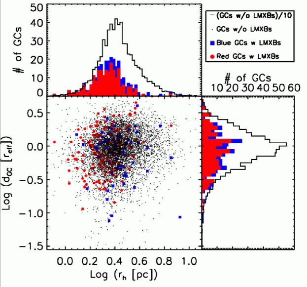
Figure 2.— GC galactocentric distances ($d_{\rm GC}$) versus observed GC half-light radii ($r_{h}$), with integrated histograms of the properties above and to the right. The symbols follow those of Figure 1. GCs that are smaller in extent are more likely to contain LMXBs. The galactocentric distance does not appear to affect whether a GC contains an LMXB.

2.3.2 Derived GC Properties

From the magnitude, colors, and radii, we can derive other parameters that might impact the formation and evolution of LMXBs in GCs. We calculate the GC mass (${M}$) directly from the $z$-band magnitude,

$${M}=\Upsilon_{z}\,10^{-0.4\,(M_{z}-M_{z,\odot})}\,{M}_{\odot}\,,$$ (1)

where $\Upsilon_{z}$ is the $z$-band mass-to-light ratio and $M_{z,\odot}=4.512$ is the absolute $z$-band magnitude of the Sun obtained from calcphot in the STSDAS Synphot IRAF package. To estimate $\Upsilon_{z}$, we use version 2.0 of the PEGASE code (Fioc & Rocca-Volmerange 1997). In PEGASE, we used the stellar initial mass function of Kennicutt (1983) to compute $(g-z)$ colors and $z$-band luminosities for an assumed age $\tau=13$ Gyr for several fixed values of [Fe/H]. Under these assumptions, $\Upsilon_{z}$ is never more than 10% different from 1.5 for [Fe/H] in the range $-2\lesssim$ [Fe/H] $\lesssim 0$, and thus $z$-band magnitudes are very good tracers of the mass. Comparably small ranges of $\Upsilon_{z}$ result if younger GC ages are assumed. Given the average $(g-z)$ of the GCs in any of our galaxies, we interpolate on these PEGASE model curves to estimate average $z$-band mass-to-light ratios. The values of $\Upsilon_{z}$ depend slightly on the mean color of the GC systems, but the variation was less than 1% across our sample galaxies when assuming that GCs are uniformly old. Thus, we chose to use a constant $\Upsilon_{z}\equiv 1.45\,{M}_{\odot}/L_{\odot}$ for all galaxies.

There is an observed correlation between $r_{h}$ and $(g-z)$, in the sense that metal-rich (red) GCs are found to be $\approx 17\%$ smaller than their metal-poor (blue) counterparts (e.g., Jordán et al. 2005). This can be a consequence of mass-segregation combined with the metallicity dependence of stellar lifetimes under the assumption that the average half-mass radius of GCs does not depend on metallicity (Jordán 2004). The observations of the size difference between metal-rich and metal-poor GCs in Virgo are consistent with this explanation (Jordán et al. 2005). Thus, it is possible that the smaller half-light radius for metal-rich GCs do not reflect a decrease in the corresponding half-mass radius $r_{h,M}$.

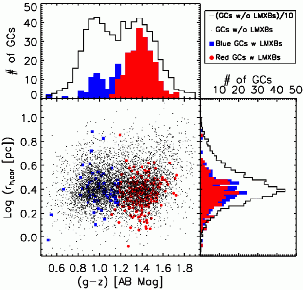
Figure 3.— Estimated GC half-light radii ($r_{h,{\rm cor}}$) versus GC colors ($g-z$), with integrated histograms of the properties above and to the right. The symbols follow those of Figure 1. There is no color dependence of $r_{h,{\rm cor}}$, indicating we have successfully removed the color dependence of half-light radius $r_{h}$. GCs that are redder and smaller in extent are more likely to contain LMXBs.

Since $r_{h,M}$ is more physically relevant in discussion of Galactic dynamics than $r_{h}$, we calculated a “corrected” half-light radius as

$$r_{h,{\rm cor}}=r_{h}\,10^{0.17[(g-z)-1.2]}=r_{h,M}\,,$$ (2)

following Jordán et al. (2005), and assume in what follows that this is the GC half-mass radius. Note that while this definition takes care of a color dependence in the half-light radii that might not reflect a corresponding dependence in the half-mass radii, $r_{h,{\rm cor}}$ can still differ from the actual half-mass radius by a constant factor (Figure 2 in Jordán 2004). We display the $r_{h,{\rm cor}}$ of the GCs in our sample in Figure 3.

Since B06 suggested that LMXBs occurred in GCs with ages greater than five times the relaxation time at the half-mass radius, $t_{h,{\rm relax}}$, we adopted the Harris (1996) corrections to Djorgovski (1993) equation (11) and used our corrected half-mass radius estimate for calculating $t_{h,{\rm relax,cor}}$:

$$t_{h,{\rm relax,cor}}=\frac{2.055\times 10^{6}}{\ln(0.4N_{*})}\,\left(\frac{\langle m_{*}\rangle}{{M}_{\odot}}\right)^{-1}\,\left(\frac{{M}}{{M}_{\odot}}\right)^{1/2}\,\left(\frac{r_{h,M}}{1{\rm\,pc}}\right)^{3/2}\,{\rm yr}\,,$$ (3)

where the average stellar mass, $\langle m_{*}\rangle$, is taken to be $\frac{1}{3}\,{M}_{\odot}$ and $N_{*}={M}/\langle m_{*}\rangle$. B06 suggested that the relaxation time be combined with the number of stars in the globular cluster to give a “stellar interaction rate” of

$$S=\frac{N_{*}}{t_{h,{\rm relax,cor}}}\,{\rm yr}^{-1}\propto{M}^{1/2}\,r_{h,M}^{-3/2}\,.$$ (4)

For a system in virial equilibrium, the relaxation time is approximately $(0.1N_{*}/\ln N_{*})\,t_{\rm cross}$, where $t_{\rm cross}$ is the stellar crossing time (roughly the orbital period of a star within the GC). Thus, $S\approx 10\ln(N_{*})/t_{\rm cross}$; except for a nearly constant factor, it is just the inverse of the orbital period. We will refer to $S$ as the “stellar crossing rate.” In Figure 4, we plot $t_{h,{\rm relax,cor}}$ versus $M_{z}$ for the GCs in our sample, overlaying lines of constant $S$ for comparison with B06, Figure 5.

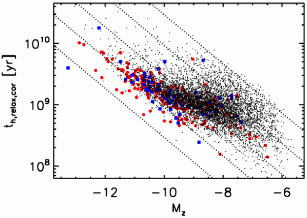
Figure 4.— GC relaxation time ($t_{h,{\rm relax,cor}}$) at half-mass versus GC magnitude ($M_{z}$), where the symbols are the same as in Figure 1. Overlaid are lines of constant stellar crossing rate ($S=N_{*}/t_{h,{\rm relax,cor}}$) that decrease by 0.5 dex starting at $\log(S\,[{\rm yr}^{-1}])=-2.5$ (lower left). The Galactic version of this plot for $V$-band is displayed in B06, Figure 5. GCs with large relaxation timescales can host LMXBs, in contrast to the result found in the much smaller sample of Galactic GCs (B06).

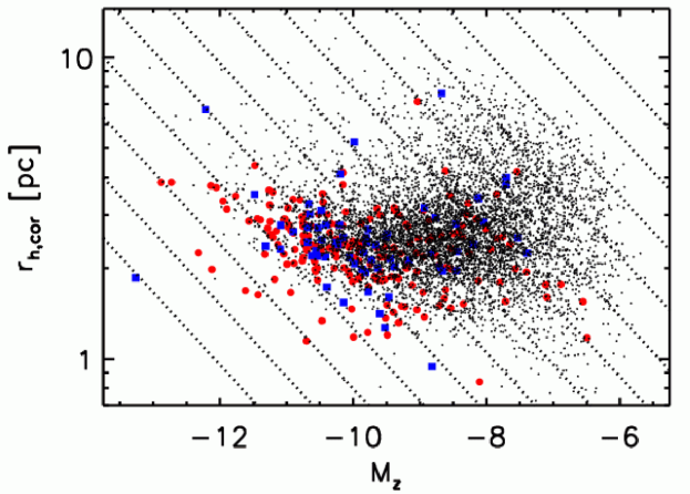
Figure 5.— Estimated GC size ($r_{h,{\rm cor}}$) versus GC magnitude ($M_{z}$), where the symbols are the same as in Figure 1. Overlaid are lines of constant encounter rate that decrease by 0.5 dex starting at $\log\Gamma_{h}=9.0$ (lower left). The Galactic version of this plot for $V$-band is displayed in B06, Figure 3. GCs with larger encounter rates are more likely to contain LMXBs.

The dynamical formation model of LMXBs in GCs is the leading explanation for the larger efficiency of LMXB production in GCs compared to the fields of galaxies. In this model, the binary is either formed by tidal capture or through exchange interactions between a NS/BH and an existing binary. In both cases, the encounter rate ($\Gamma$) is thought to depend on the properties of GCs at their cores; $\Gamma\propto\rho_{0}^{3/2}r_{c}^{2}$, where $\rho_{0}$ is the central density, $r_{c}$ is the core radius, and the virial theorem has been assumed to connect core velocities to densities and radii (see, e.g., Verbunt 2003). Although these parameters are not directly measurable at the distance of the Virgo cluster, we can create a proxy,

$$\Gamma_{h}\equiv\left(\frac{{M}}{2\pi{M}_{\odot}}\right)^{3/2}\,\left(\frac{r_{h,M}}{1\,{\rm pc}}\right)^{-5/2}\,,$$ (5)

where we have assumed that the relation between core structural parameters and the parameters at a half-mass radius (dictated by the concentration, $c$) is the same for all GCs. The latter assumption is not necessarily true, e.g. there is an observed trend in Galactic GCs for the concentration to increase with GC mass (McLaughlin 2000). In any case, we define $\Gamma_{h}$ to be our tracer for encounter rates under the assumptions stated; our results on the dependence of the expected number of GC LMXBs on $\Gamma_{h}$ can be easily compared with theoretical predictions based on any alternate assumptions. We note that if GCs with higher concentrations are more likely to contain LMXBs, then the $\Gamma_{h}$ we calculate will underpredict the encounter rate for GCs with LMXBs. We plot $r_{h,{\rm cor}}$ versus $M_{z}$ for GCs in our sample, overlaying lines of constant $\Gamma_{h}$, in Figure 5 for comparison with B06, Figure 3.

ACSVCS3 used measured King models concentrations $c$ to estimate $\Gamma$ directly. As the measured $c$ are rather uncertain for most sources, we prefer to use $\Gamma_{h}$ in this work. We note though that the results of ACSVCS3 are robust with respect to uncertainties in the measured $c$; indeed all conclusions remain unchanged if a single $c\equiv 1.5$ is assumed for all GCs. In other words, their conclusions remain the same when using $\Gamma_{h}$ rather than $\Gamma$.

2.4. Matching LMXBs And GCs

To determine the relative astrometry between CXO and HST observations for each galaxy, we convolved the offset positions in RA and Dec between all X-ray and optical positions with a $\sigma=0\farcs 5$ 2-dimensional Gaussian, which approximates the PSF of CXO, to create a cross-correlated image. The maximum cross-correlation was used to determine the astrometric offset. After correcting for this offset, X-ray sources within $1\arcsec$ of optical sources were considered to be matched. We chose $1\arcsec$ as a balance between accurate identification of the X-ray source astrometry (the astrometric accuracy of CXO in the small count regime is $\sim 0.3$–$0.5\arcsec$) and the increased number of falsely identified sources with larger match radii.

If an X-ray source was matched to both non-GC optical sources (e.g., background galaxies) and GCs, we excluded the X-ray source and GCs from our analysis. All remaining 288 X-ray detections in GCs were considered to be GC-LMXBs. For the 18 GC-LMXBs that were within $1\arcsec$ of multiple GCs, we could not determine which GC contained the LMXB; however, if the multiple GCs all belonged to the same sub-population (blue-GC vs. red-GC), we could count the GC-LMXB as belonging to that sub-population. We indicate the number of GCs with LMXBs, and separately list the numbers of LMXBs in blue-GCs and red-GCs, in the eighth, ninth, and tenth columns of Table 3. In parenthesis, we indicate the number of GC-LMXBs matched to multiple GCs. We also indicate the corresponding number of GCs in the brackets of columns four, six, and seven.

We separated the GCs into two sub-populations, those that clearly contained an LMXB in our Detected sample (indicated by a subscripted $X$), and those that clearly did not (indicated by a subscripted $nX$). We found 270 GCs that contained an LMXB at our detection levels and 6,488 GCs that clearly did not. We display the properties of these GCs in Figures 1–4, indicating blue-GCs with LMXBs using filled blue squares and red-GCs with LMXBs using filled red circles. Of the 270 GCs clearly containing an LMXB, 160 are in the SNR sample, and 61 are in the Complete sample.

We randomized the position angles of the GCs around the centers of their host galaxies to estimate the number of LMXBs falsely associated with GCs. We adopted two different methods: either we kept the galactocentric distance of the GC fixed, or we assumed that the GC lay on the same elliptical isophote on which it was originally detected. We reassessed the matches with the randomized GC catalogs, and used the number of resulting matches to predict the percentage of non-GC X-ray sources falsely matched to a GC, $p_{\rm false}$. Since there was typically little difference between the two methods, we averaged the two. Given the typical values of these numbers ($3.3$–$14.8\%$), it is unlikely that any of the GC-LMXBs matched to multiple GCs are not actually associated with a GC; however, some fraction of the GC-LMXBs matched to a single GC will be false matches. The predicted number of falsely matched sources is $p_{\rm false}/(1-p_{\rm false})$ times the number of observed non-GC X-ray sources. The term in the denominator accounts for the falsely matched sources removed from the non-GC X-ray sample. The expected number of false matches is displayed in the eleventh column of Table 3. The large GC density in NGC 4486 leads to a correspondingly larger number of false matches; however, the number of false matches still make up less than $15\%$ of the identified GC-LMXBs. With the number of false GC-LMXBs and total number of GCs, we estimate the expected number of false matches per GC, $\lambda_{f}$, for each galaxy, which range from about $2\times 10^{-3}$ to $7\times 10^{-3}$.

3. Properties of GCs with and without LMXBs

In what follows we compare the properties of GCs that harbor an LMXB with those of GCs that do not harbor one. We probe in turn the distributions of luminosity (mass), $(g-z)$ color (metallicity), size ($r_{h}$), galactocentric distance, half-mass relaxation time $t_{h,\rm rel}$ and dynamical rates $S$. By revealing which properties drive the presence of an LMXB in GCs – or which ones are irrelevant – this exercise can shed light on the formation process of LMXBs in GCs.

We employ three methods to compare the properties of GCs with and without LMXBs (When comparing the properties of the SNR sample and Complete sample to GCs without LMXBs, we did not add the GCs which had LMXBs that did not fall in the sample into the sample of GCs without LMXBs.) First, we use binned histograms of various properties to display the qualitative differences. These histograms are displayed in Figures 1–4. Second, we calculate the median values of the GC properties and use the non-parametric Wilcoxon rank-sum test ($\sigma_{\rm WRS}$, equivalent to the Mann-Whitney rank-sum test; Mann & Whitney 1947) to quantify the differences. We additionally use the Wilcoxon test to compare the properties of GCs with LMXBs in the Complete sample and GCs with LMXBs fainter than the Complete sample limit. Finally, we bin the GCs by the different parameters available and look for non-uniform probabilities of GCs containing an LMXB. The results of the latter exercise are shown in Figure 6. The errors on the fractions in Figure 6 are calculated assuming Poisson statistics (i.e., strict 1$\sigma$ confidence intervals were calculated as opposed to using the $\sqrt{N}$ approximation). The fractions in Figure 6 were corrected for the rate of false matches, $\lambda_{f}$.

Figure 6.— The percentage of GCs containing an LMXB as a function of GC magnitude ($M_{z}$), color ($g-z$), half-mass radius ($r_{h,{\rm cor}}$), and galactocentric distance ($d_{\rm GC}$). GCs that are brighter, are redder, and have smaller half-mass radii are more likely to contain LMXBs. The uncertainties are at the 1$\sigma$ confidence level. The bins were set by requiring 27 GCs with LMXBs per bin.

3.1. Luminosity and Mass

Prior observations have revealed that more luminous GCs appear to preferentially host LMXBs (e.g., Angelini et al. 2001; Kundu et al. 2002; Sarazin et al. 2003; Jordán et al. 2004b). Figure 1 confirms that LMXBs are found more often in brighter GCs. The median $M_{z}$ is $-8.5$ for GCs without LMXBs, and $-9.9$ for GCs with LMXBs (all samples), which correspond to Wilcoxon rank-sum differences of 15.6$\sigma$ (Detected sample), 11.8$\sigma$ (SNR sample), and 6.6$\sigma$ (Complete sample). We find no significant difference ($\sigma_{\rm WRS}=0.9$) in the optical luminosities of GCs in the Complete sample and of GCs with fainter LMXBs.

The median mass of a GC with an LMXB is 3.6 times that of a GC without an LMXB. The upper left panel of Figure 6 suggests a power-law dependence of the probability of a GC containing an LMXB on the mass of the GC.

3.2. Color

Prior observations also have revealed that redder GCs appear to preferentially host LMXBs (e.g., Kundu et al. 2003; Sarazin et al. 2003; Jordán et al. 2004b). Our larger sample clearly confirms this (see Figure 1). The median $(g-z)$ color is 1.20 for GCs without LMXBs, and 1.34 (Detected sample), 1.35 (SNR sample), and 1.38 (Complete sample) for GCs with LMXBs, which correspond to Wilcoxon rank-sum differences of 6.6$\sigma$, 5.8$\sigma$, and 3.7$\sigma$. There were no significant differences ($\sigma_{\rm WRS}=1.2$) in the colors of GCs in the Complete sample and GCs with fainter LMXBs.

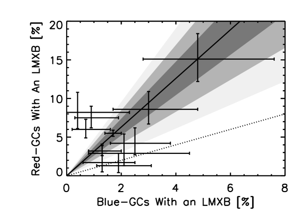
Figure 7.— The percentage of red-GCs containing an LMXB versus the percentage of blue-GCs containing an LMXB for the Detected sample. The data points with 1$\sigma$ confidence limits are the different galaxies in our sample. The dotted line indicates the cumulative relation that red-GCs contain as many LMXBs as blue-GCs; the data clearly do not support this relation. The solid line indicates the cumulative relation that red-GCs contain $3.15\pm 0.54$ times as many LMXBs as blue-GCs. The greyscale indicates the area covered by 1, 2, and 3$\sigma$ off of the best fit.

Previous works have often compared the fraction of blue-GCs with LMXBs to the fraction of red-GCs with LMXBs, and found that red-GCs are $\sim 3$ times more likely to contain LMXBs that their blue counterparts. In Figure 7, we compare these fractions computed using the Detected sample. The cumulative sample suggests that red-GCs are $3.15\pm 0.54$ times more likely to have LMXBs than blue-GCs; however, there is considerable scatter in this fraction between galaxies.

The upper right panel of Figure 6 suggests that the probability that a GC contains an LMXB depends exponentially on the color. Based on the observed color distribution bimodality, some GC formation scenarios posit that the red and blue GC subpopulations have different formation histories (see, e.g., West et al. 2004). If the presence of an LMXB in a GC was somehow mainly determined by this history, it is conceivable that the probability of a GC holding an LMXB was different for each subpopulation but independent of color within each subpopulation. If this dependence were due only to a difference between the red and blue GC populations, but were independent of the color of a GC within the two populations, this would appear as a step-function relation in the upper right panel of Figure 6, except for the third bluest color bin. This bin contains all but two of the different galactic division points between red-GCs and blue-GCs. As such, its value would be intermediate between the two efficiencies. Since both pictures, i.e., a continuous exponential dependence and a step-function, have two constraints, we can compare their $\chi^{2}$ fits to test which interpretation is more consistent with the data. For these fits, we always excluded the third bluest color bin and tested the effect of excluding zero, one, or two of the reddest color bins. Since the step-function model always had a higher $\chi^{2}$ compared to the exponential function model ($\chi^{2}_{\rm step}/{\rm dof}=12.8/6,12.8/5,{\rm\,and\,}6.2/4$ compared to $\chi^{2}_{\rm exp}/{\rm dof}=9.7/6,6.0/5,{\rm\,and\,}3.7/4$, respectively), we do not believe that the probability that a GC contains an LMXB depends on a difference between the red and blue GC populations that is independent of the color of a GC within the two populations. Since color is roughly a logarithm of metallicity, we prefer interpreting the upper right panel of Figure 6 as an indication that the probability a GC contains an LMXB has a continuous power-law dependence on GC metallicity.

3.3. Size

Although there were indirect indications that the size of GCs affect the formation or evolution of LMXBs in ACSVCS3, we present here the first explicit evidence of this. We find that LMXBs are found more often in GCs that have smaller half-light radii (Figure 2). Because the half-light radii of GCs are uncorrelated with their mass (McLaughlin 2000; Jordán et al. 2005), this implies that LMXBs are found more often in GCs that are denser. The median $r_{h}$ values are $2.6{\rm\,pc}$ for GCs without LMXBs, and $2.3{\rm\,pc}$ (Detected sample), $2.3{\rm\,pc}$ (SNR sample), and $2.2{\rm\,pc}$ (Complete sample) for GCs with LMXBs, which correspond to Wilcoxon rank-sum differences of 8.1$\sigma$, 7.4$\sigma$, and 4.9$\sigma$. Although the differences in the medians are $\lesssim 15\%$, the distributions are found to be significantly different for two reasons. First, with the number of GCs in our samples, the Wilcoxon test is sensitive to 10%, 14%, and 22% differences in the medians, respectively, at the 3$\sigma$ level. Second, the Wilcoxon test samples the entire distribution, not just the medians. For example, the values of the half-light radii that contain 90% of the GCs are $4.3{\rm\,pc}$ for GCs without LMXBs, and $3.3{\rm\,pc}$ (Detected sample), $3.0{\rm\,pc}$ (SNR sample), and $3.0{\rm\,pc}$ (Complete sample) for GCs with LMXBs. Kolmogorov-Smirnov tests indicate that the probability the distributions of half-light radii are drawn from the same sample are $5.7\times 10^{-13}$ (Detected sample), $8.1\times 10^{-11}$ (SNR sample), and $9.6\times 10^{-6}$ (Complete sample), consistent with the Wilcoxon tests. Once again, we found no significant differences ($\sigma_{\rm WRS}=1.2$) in the half-light radii of GCs in the “Complete sample” and GCs with fainter LMXBs.

Given that redder GCs are more likely to contain LMXBs and have smaller half-light radii, we also compared the half-mass radii (see eq. [2]) of GCs with and without LMXBs (Figure 3). Our adopted half-mass radii should be, by definition, nearly insensitive to color variations. The median $r_{h,{\rm cor}}$ of GCs with LMXBs were only $0.1{\rm\,pc}$ more than their half-light radii. The distributions of half-mass radii of GCs with and without LMXBs are different at the 5.9$\sigma$ (Detected sample), 5.5$\sigma$ (SNR sample), and 3.7$\sigma$ (Complete sample) levels according to the Wilcoxon rank-sum test. Thus, GCs that are smaller in extent remain more likely to contain LMXBs, even if the half-mass radii are used to measure the size.

The lower left panel of Figure 6 suggests that the probability that a GC has an LMXB may decrease roughly as a power-law of the half-light radius. There is a similar, but slightly flatter dependence on half-mass radius.

3.4. Galactocentric Distance

Kim et al. (2006) present a study of LMXBs in six early-type galaxies (four overlap with our study). Combining HST-WFPC2 and ground-based observations they identify 285 LMXBs with GCs. They find that LMXBs are more likely (at the $6.6\sigma$ significance level) to be found in GCs in the inner $0.5d_{\rm eff}$ compared to an annulus between one-half and one times the isophotal $B=25{\rm\,mag\,arcsec}^{-2}$ radius; 44 GC-LMXBs out of 1004 GCs are found in the inner region versus 69 GC-LMXBs out of 2908 GCs in the outer). The suggest their results indicate that galactocentric distance plays a critical role and that GCs may have more compact cores near the galactic center, and thus higher encounter rates.

The effect of galactocentric distance on the probability that a GC has a LMXB is less clear in our data. For comparison with their result, we examine the same inner annulus and $1.5d_{\rm eff}<d<3.0d_{\rm eff}$, which corresponds to approximately the same outer annulus. We find 66 GC-LMXBs out of 1211 GCs versus 44 GC-LMXBs out of 1203 GCs. Although the inner region is numerically more likely to have GCs containing LMXBs in our sample, this result is not statistically significant ($1.7\sigma$). Comparing the inner regions of the two samples, where their study relies heavily on HST identifications, are clearly consistent. There is a large discrepancy in the outer region. With ground-based (and to a much lesser extent HST-WFPC2 observations), it is more likely that contamination of GCs with unrelated objects occurs when compared with our HST-ACS observations. Although Kim et al. (2006) attempt to account for this contamination, underestimation of the contamination level would result in a larger falsely identified GC population that would deflate their measured likelihood of finding a GC with an LMXB in the outer field.

In our data, the values of $d_{\rm GC}$ are slightly smaller for GCs with LMXBs in the Complete sample as compared to GCs with LMXBs not in the Complete sample, but the difference is not very significant ($\sigma_{\rm WRS}=2.2$). This could indicate that the values of $d_{\rm GC}$ are affected by incompleteness. Since the incompleteness is more important in the X-ray brighter, central regions of galaxies, and incompleteness affects the fainter LMXBs more, this effect is not unexpected. There is no significant difference ($\sigma_{\rm WRS}=1.6$) in the radial distributions between the Detected sample of GCs with LMXBs and GCs without LMXBs; however, there are slightly significant differences when using the SNR sample ($\sigma_{\rm WRS}=3.1$) and Complete sample ($\sigma_{\rm WRS}=2.8$). The lower right panel of Figure 6 suggest that there may be a slight decrease with $d_{\rm GC}$ in the probability that a GC contains an LMXB. However, since red-GCs tend to be closer to the galaxy center and are more likely to contain LMXBs, it is possible that the lower galactocentric distances of GCs with LMXBs in the SNR and Complete sample can be completely accounted for without invoking an intrinsic difference in the probability a GC contains an LMXB on $d_{\rm GC}$. Given the marginal, if any, strength of the dependence on $d_{\rm GC}$, we do not consider it further in this paper. We have however checked that including a galactocentric distance effect does not alter any of our scientific conclusions.

3.5. Relaxation Time

No Galactic GC with a relaxation timescale $\gtrsim 2.5{\rm\,Gyr}$ contains an active LMXB (B06). Their Galactic sample is limited to 141 GCs, 12 of which contain LMXBs with $L_{X}>10^{35}{\rm\,erg\,s}^{-1}$. Our sample, which does not probe as deeply in X-ray luminosity, includes 6,758 GCs, 270 of which contain LMXBs. In our much larger sample (Figure 4), about 18% of the GCs with LMXBs have relaxation timescales larger than this. We used Monte Carlo simulations to estimate that measurement errors only bias this result by about 3%. In other words, the relaxation timescale of about 15% of the GCs are intrinsically larger than 2.5 Gyr. The relaxation timescale of the GCs with LMXBs in our sample are larger than those GCs without LMXBs; the median $t_{h,{\rm relax,cor}}$ is $1.0{\rm\,Gyr}$ for GCs without LMXBs, and $1.5{\rm\,Gyr}$ (Detected sample), $1.4{\rm\,Gyr}$ (SNR sample), and $1.3{\rm\,Gyr}$ (Complete sample) for GCs with LMXBs. This difference is opposite to that seen in the Galaxy, where the median $t_{h,{\rm relax}}$ are $0.7{\rm\,Gyr}$ for GCs with LMXBs and $1.3{\rm\,Gyr}$ for GCs without LMXBs (Harris 1996). In our sample, the relaxation timescale distributions of GCs with LMXBs are different from GCs without LMXBs at the 6.8$\sigma$, 4.6$\sigma$, and 2.4$\sigma$ level according to the Wilcoxon rank-sum test; the equivalent test on Galactic GCs indicates a difference of 2.0$\sigma$. We found no significant differences ($\sigma_{\rm WRS}=1.3$) between the half-mass relaxation timescales of GCs in the “Complete sample” and GCs with fainter LMXBs.

3.6. Dynamical Rates

There are two dynamical rates that could affect formation or evolution of LMXBs: the stellar crossing rate ($S\propto{M}^{1/2}\,r^{-3/2})$ and the encounter rate ($\Gamma_{h}\propto{M}^{3/2}\,r^{-5/2}$). Since GCs that are more massive and smaller in extent are more likely to contain LMXBs, it is clear that both of these rates would be higher in GCs with LMXBs compared to GCs without LMXBs (Fig. 5 and 4). The median values of $S$ are $0.74{\rm\,kyr}^{-1}$ for GCs without LMXBs and $1.8{\rm\,kyr}^{-1}$ (Detected sample), $2.0{\rm\,kyr}^{-1}$ (SNR sample), and $1.8{\rm\,kyr}^{-1}$ (Complete sample) for GCs with LMXBs, corresponding to 16.9$\sigma$, 13.3$\sigma$, and $7.8\sigma$ Wilcoxon rank-sum differences. For $\Gamma_{h}$, the median values are $6.9\times 10^{5}$ for GCs without LMXBs and $7.3\times 10^{6}$ (Detected sample), $7.9\times 10^{6}$ (SNR sample), and $6.4\times 10^{6}$ (Complete sample) for GCs with LMXBs, corresponding to 17.1$\sigma$, 13.2$\sigma$, and $7.7\sigma$ Wilcoxon rank-sum differences. We found no significant differences ($\sigma_{\rm WRS}=0.1$) between either of the dynamical rates of GCs in the Complete sample and GCs with fainter LMXBs.

4. Multi-Variable Relation Between LMXBs and GCs

4.1. Technique

Since several properties appear to affect the probability that a GC contains an LMXB, it is important to simultaneously account for these properties. Based on Figure 6 and the relatively small percentage of GCs falsely matched to LMXBs $\lambda_{f}$, we have assumed the expected (true) number of LMXBs in a GC ($\lambda_{t}$) has the following dependence on GC properties:

$$\lambda_{t}=A\,\left(\frac{{M}}{{M}_{\odot}}\right)^{\beta}\,10^{\delta\,(g-z)}\,\left(\frac{r}{1{\rm\,pc}}\right)^{\epsilon}\,,$$ (6)

where we fit for the normalization ($A$) and indices ($\beta$, $\delta$, and $\epsilon$). Here, $r$ can either be the measured half-light radius $r_{h}$ or the corrected half-mass radius $r_{h,{\rm cor}}$. Our approach differs from the fitting performed in ACSVCS3; we choose to fit the expected numbers of LMXBs per GC, as opposed to the probability a GC contains an LMXB. The probability must saturate at unity, whereas the expected number can be unlimited; this makes it easier to fit simple functions (e.g., power-laws) to the expected number and compare with Galactic results. The two approaches give the same results when $\lambda_{t}$ is small. By including the normalization $A$ we get a direct estimate for the number of LMXBs in GCs and we are able to probe quantitatively the fraction of GC X-ray point sources that are expected to result from the integrated X-ray flux of multiple sources. Another difference is that we include a term to account for GCs falsely matched to LMXBs, $\lambda=\lambda_{f}+\lambda_{t}$.

The expected number of LMXBs in a GC can be converted to a probability that there are no LMXBs assuming a Poisson distribution,

$$P_{nX}=\exp(-\lambda)\,,$$ (7)

and the probability that there is at least one LMXB,

$$P_{X}=1-\exp(-\lambda)\,.$$ (8)

One can then vary the parameters to maximize the log likelihood,

$$\psi=\ln\left[\left({{\displaystyle\prod}\atop{\scriptstyle nX}}P_{nX}\right)\,\left({{\displaystyle\prod}\atop{\scriptstyle X}}P_{X}\right)\right]\,,$$ (9)

where the products are taken over the lists of GCs with no LMXBs and GCs with LMXBs. Given that we did not find a difference in the masses, colors, or sizes of GCs with LMXBs in the Complete sample as compared to those GCs with fainter LMXBs, we first choose to use the better statistics provided by the Detected sample to fit the indices. Given the widely different luminosity limits in the Detected sample, we do not believe the normalization we fit is physically meaningful. To derive a physically meaningful normalization, we apply our derived exponents to the Complete sample. Since the log likelihood can be related to $\Delta\chi^{2}$, ($-2\Delta\psi=\Delta\chi^{2}$), we use the change in log likelihood for one degree of freedom (dof) to determine one-dimensional fitting errors (1$\sigma$) on each varying parameter.

Table 4Fits of the Expected Number $\lambda_{t}$ of LMXBs per GC

	$\lambda_{t}\propto{M}^{\beta}\,10^{\delta\,(g-z)}\,r^{\epsilon}$
Row	$\beta$	$\delta$	$\epsilon$	$\psi$	$\Delta$ dof
$r=r_{h}$
1	$[0]$	$[0]$	$[0]$	-1131.1	0
2	$1.027^{+0.063}_{-0.061}$	$[0]$	$[0]$	0-986.0	1
3	$[0]$	$0.64^{+0.12}_{-0.11}$	$[0]$	-1113.5	1
4	$1.009^{+0.060}_{-0.059}$	$0.77^{+0.13}_{-0.13}$	$[0]$	0-967.2	2
5	$[0]$	$[0]$	$-1.50^{+0.20}_{-0.20}$	-1101.2	1
6	$1.237^{+0.076}_{-0.075}$	$0.52^{+0.15}_{-0.15}$	$-2.22^{+0.24}_{-0.25}$	0-918.4	3
$r=r_{h,{\rm cor}}$
7	$[0]$	$[0]$	$-1.14^{+0.20}_{-0.21}$	-1113.6	1
8	$1.237^{+0.076}_{-0.075}$	$0.90^{+0.15}_{-0.14}$	$-2.22^{+0.24}_{-0.25}$	0-918.4	3

We display the results of our fits to the Detected sample in Table 4, where bracketed numbers indicate that an index was frozen to that number. Once a form for $\lambda_{t}$ as a function of mass, color, and radius has been determined, we can use this expectation to predict the fraction of GCs having an LMXB as a function of each of the GC properties. These predictions can be compared to the plots of the variation of this probability with individual properties shown in Figure 6. For each of the binned data points in each of the panels of this Figure, we apply the best-fit expectation calculated for each of the other properties of the GCs in the binned data point, and then compute the expected fraction integrated over that bin. This is compared to the actual fraction for the bin, and the contribution to $\chi^{2}$ from that bin is determined. Since we do not consider the dependence of $\lambda_{t}$ on galactocentric distance, we did not include that panel’s contribution to $\chi^{2}$. Since the $\chi^{2}$ of that panel ranged from 4.2–11.4 for 10 dof for all fits in Table 4, this is justified. In this way, we can determine whether the best-fit expectation function fits the binned data in Figure 6 adequately. The results, which we describe in detail in what follows, are shown in Figures 8 and 9.

Figure 8.— Identical to Figure 6, except with the results of fitting the dependence of the expected number of LMXBs on GC mass and color (Table 4, row 4) overlaid. Note that fitting the effects of mass and color alone does not reproduce the observed dependence of the probability on radius or color very well.

Figure 9.— Identical to Figure 6, except with the results of fitting the dependence of the expected number of LMXBs on GC mass, color, and half-mass radius (Table 4, row 8) overlaid. Note that simultaneously fitting the effects of GC mass, color, and half-mass radius reproduces the observed dependence of the probability on all of the observed parameters reasonably well.

4.2. Effect of GC Mass and Color

We first established a baseline assuming that the expected number of LMXBs per GC has no dependence on GC properties (Table 4, row 1); our binned $\chi^{2}$ was 402.4 for 29 dof ($3\times 10$ data points minus one constraint for the normalization). We next individually varied the mass and color indices (Table 4, rows 2 and 3); mass clearly had the largest effect ($-2\Delta\psi=290.2$); however, its binned $\chi^{2}$ was still as large as 158.6 for 28 dof. If we included the effects of mass and color simultaneously (Table 4, row 4), we had a much improved fit from the mass-only fit ($-2\Delta\psi=37.6$). We display this fit in Figure 8, which has a binned $\chi^{2}$ of 106.4 for 27 dof. Although the effect of color on $\lambda_{t}$ was included in this fit, the resulting expression does not provide a very good fit to the dependence of the fraction on color alone (Figure 8, upper right panel). The $\chi^{2}$ is 26.5 for 10 bins in this figure. In general, the dependence of $\lambda_{t}$ on mass and color does not adequately describe the observed number of LMXBs per GC as a function of the observed GC properties. Some dependence on another GC property is required.

We note that based on known correlations of GC properties we do not expect a relation based on GC mass and color alone to be able to reproduce any dependence on GC size. Namely, the mean $r_{h}$ of GCs is observed to be independent of mass (McLaughlin 2000; Jordán et al. 2005) and our $r_{h,\rm cor}$ has no dependence on color. Thus, any dependence of $\lambda_{t}$ on $r_{h,\rm cor}$, as observed in the lower left panel of Figure 6, cannot be reproduced by a function which depends only on GC mass and color.

In the prior largest sample of GCs with LMXBs to date (6 galaxies, 98 LMXBs in 2,276 GCs), Smits et al. (2006) found $P(LMXB)\propto{M}^{1.03\pm 0.12}\,{Z}^{0.25\pm 0.03}$. Since they used multiple color indices, they adopted linear color-metallicity relations based on Milky Way GCs, ignoring scatter in the relation. For comparison with their data, we adopt the linear color-metallicity relation presented in ACSVCS3 $(g-z)\sim 0.38\rm{[FE/H]}+1.62$. In that case, we derive $\lambda\propto{M}^{1.009^{+0.060}_{-0.059}}{Z}^{0.29\pm 0.10}$, which is consistent with their results. However, as we point out in the next section, the effect of GC sizes must be taken into account. This effect alters the measured indices for mass and color, which will in turn alter interpretations based on those indices.

4.3. Effect of GC Size

There are two GC sizes we considered in our fits: the half-light radius ($r=r_{h}$), and the half-mass radius ($r=r_{h,{\rm cor}}$). Fitting half-light radius alone (Table 4, row 5) leads to a better fit than fitting color alone; however, given the correlation between color and half-light radius, it is not clear if this is due in part to the dependence on color or a real dependence on the cluster size. On the other hand, only fitting the half-mass radius (Table 4, row 7) is nearly equivalent to only fitting the color (row 3). This is consistent with the picture developed from the Wilcoxon tests presented in § 3.

4.4. Simultaneous Effect of GC Mass, Color, and Size

The best fits come from simultaneously fitting the effects of mass, color, and radius (Table 4, rows 6 and 8). Compared to just fitting the effects of mass and color, the fits are greatly improved ($-2\Delta\psi=97.6$), and the binned $\chi^{2}$ values are reasonable (20.2 for both half-light radius and half-mass radius with 26 dof). Regardless of which size is chosen, the mass and radius exponents are the same. The addition of the radius actually increases the mass exponent beyond the fitting errors one derives if radius is ignored. The color index also differs when size is ignored. If the half-light radius is used, one finds a smaller index; however, we believe the correlation between half-light radius and color affects this fit, so that this does not give an accurate view of the dependence on the size of the cluster. When the half-mass radius is used, one finds a larger index; however, the increase is only at a $\sim$1$\sigma$ level. The sizes of GCs play a critical role in not only affecting the number of LMXBs per GC, but also our interpretation of how strongly GC mass and color affect the number of LMXBs per GC.

We believe that the simultaneous fitting of GC masses, colors, and half-mass radii provide the most physically motivated fit of the LMXB-GC connection. For this fit (Figure 9), we derive $\beta=1.237^{+0.076}_{-0.075}$, $\delta=0.90^{+0.15}_{-0.14}$, and $\epsilon=-2.22^{+0.31}_{-0.36}$. We note that by including the effect of GCs falsely matched to LMXBs we increased the mass exponent by 13%, increased the color index by 16% and decreased the radius exponent by 16%.

If we require that the expected number of LMXBs scales linearly with the mass ($\beta\equiv 1$), the negative log-likelihood function is increased by $-2\Delta\psi=10.7$ for 1 more dof, and the binned $\chi^{2}$ is 30.9 for 27 dof. Thus, we rule out a linear proportionality of mass at the 99.89% confidence limit. We discuss the implications of this in the next subsection.

From Figure 9, we see that the declining probability for a GC with $(g-z)>1.4$ to contain an LMXB can be reproduced although we assume no break in the relation between color and $\lambda$. This suggests that the masses and half-mass radii of GCs at these colors may be different than at bluer colors. Indeed, the fraction of GCs with $r_{h}\gtrsim 3$ pc increases systematically with color for $(g-z)>1.4$. One possible explanation is contamination by diffuse stellar clusters, which are redder, fainter cousins of GCs (e.g., Larsen & Brodie 2000; Peng et al. 2006b). Additionally, we note that the small variations of the probability with galactocentric distance are reproduced, even though the distance played no role in the fit.

We used the indices from our best-fit to the Detected sample to determine the normalization for the Complete sample:

$$\lambda_{t}=8.0\times 10^{-2}\,\left(\frac{{M}}{10^{6}\,{M}_{\odot}}\right)^{1.237}\,10^{0.90\,(g-z)}\,\left(\frac{r_{h,{\rm cor}}}{1{\rm\,pc}}\right)^{-2.22}\,.$$ (10)

Since our method predicts the expected number of LMXBs per GC, we can determine the likelihood that a GC would contain multiple LMXBs. Note that M15 in our Galaxy has two active LMXBs (White & Angelini 2001); however, the LMXBs in M15 have $L_{X}\sim 10^{36}{\rm\,erg\,s}^{-1}$ and would not be detected at the distances of the galaxies in our sample. We calculate the number of GCs containing multiple LMXBs, $N_{\rm mult}$, as

$$N_{\rm mult}=\sum_{X,nX}[1-(1+\lambda_{t})e^{-\lambda_{t}}],$$ (11)

obtaining $N_{\rm mult}=1.3$. Normalizing this to the number of GCs with LMXBs in the Complete sample (61), we estimate that $2.2^{+3.9}_{-1.7}\%$ of GCs with LMXBs actually contain multiple LMXBs such that their combined luminosity is above $3.2\times 10^{38}{\rm\,erg\,s}^{-1}$. This fraction should increase as the LMXB luminosity limit of the sample decreases. For example, the same calculation for our Detected sample with lower luminosity LMXBs gives an expected fraction of $8.2^{+2.0}_{-1.7}\%$ of GCs with multiple LMXBs.

4.5. Implications of Simultaneous Fit

For multivariate datasets, principal component analysis determines the set of orthogonal eigenvectors, linear combinations of the original variables, that minimize the Euclidean distances to each eigenvector (e.g., Murtagh & Heck 1987). The normalized variances of the data projected onto the eigenvectors, the eigenvalues, are used to order the eigenvectors. The eigenvectors with larger eigenvalues are the best-fit eigenvectors to the data. Often, only eigenvectors with eigenvalues greater than unity (i.e., those eigenvectors that are as good fits as the original variables) are retained. Principal component analysis among the masses, colors, and radii of GCs with LMXBs found two eigenvectors whose eigenvalues were above unity. The first eigenvector has an eigenvalue of 1.22 and is dominated by an approximately equal combination of mass and half-mass radius, while the second eigenvector has an eigenvalue of 1.01 and is dominated by color. Therefore, we break our interpretation of the fits into two parts: an interpretation of the variation with color as a metallicity effect, and a discussion of the combined mass and half-mass radius variation as evidence for the dynamical formation of LMXBs in GCs.

4.5.1 Metallicity Effect on the Presence of LMXBs

We find a monotonic increase in the expected number of LMXBs with GC color of the form $\lambda_{t}\propto 10^{0.90^{+0.15}_{-0.14}(g-z)}$. Using data from NGC 4486, ACSVCS3 found that the probability that a GC contains an LMXB is $P_{X}\propto 10^{0.87^{+0.22}_{-0.22}(g-z)}$. For small values of the expected number ($\lambda_{t}\ll 1$), these two quantities are nearly identical ($P_{X}\approx\lambda_{t}$, eqn. [8]). Thus, our slightly different techniques are in good agreement with respect to the fit to color variation. In ACSVCS3, the color variation was directly converted into a metallicity variation by applying the Bruzual & Charlot (2003) models, which give $(g-z)\sim(0.38\pm 0.05)\log\frac{{Z}}{{Z}_{\odot}}$ and therefore $P_{X}\propto{Z}^{0.33\pm 0.1}$. In this paper, we converted color to metallicity following equation (2) of Peng et al. (2006a),

$$\log\frac{{Z}}{{Z}_{\odot}}=\left\{\begin{array}[]{cc}-6.21+(5.14\pm 0.67)(g-z)&{\rm for\ }g-z\leq 1.05\,;\\ -2.75+(1.83\pm 0.23)(g-z)&{\rm for\ }g-z>1.05\,.\end{array}\right.$$ (12)

We then replaced the $10^{(g-z)\delta}$ term from equation 6 with $({Z}/{Z}_{\odot})^{\delta^{\prime}}$. We find $\delta^{\prime}=0.391^{+0.070}_{-0.067}$, with no change to the variation with mass or radius. The dependence on ${Z}$ we find here is consistent with that found in ACSVCS3 and with recent results on the metallicity dependence of the production of likely quiescent LMXBs in Galactic GCs (Heinke et al. 2006). Compared to fitting the effect of mass, radius, and color, the mass, radius, and metallicity fit is very slightly worse ($-2\Delta\psi=2.0$); however, the binned $\chi^{2}$ value is still reasonable (20.3 for half-mass radius, both with 26 dof).

There are several ideas that could explain the relation between metallicity and the likelihood that a GC will contain an LMXB, most of which were summarized in ACSVCS3. First, metal-rich stars may have larger radii and masses compared to metal-poor stars (Bellazzini et al. 1995), which would make it easier to form LMXBs. This would increase both the number of Roche-lobe overflow systems and the number of binary systems formed. Following Maccarone et al. (2004), we have estimated that the number of Roche-lobe overflow systems has a weak metallicity dependence, ${Z}^{0.11}$. The number of NS binaries formed by tidal capture goes as ${Z}^{0.12}$, but may have a lower exponent for exchange interactions. Thus, this model predicts a ${Z}^{\lesssim 0.2}$ dependence and is inconsistent with our fit.

Ivanova (2006) suggested that the link between metallicity and outer convective zones was responsible for the increased formation efficiency of LMXBs in metal-rich GC. In this model, metal-poor main-sequence stars lack an outer convective zone. This absence turns off magnetic braking. Since magnetic braking leads to the strong orbital shrinkage that eventually leads to mass transfer as an LMXB, metal-poor stars fail to dynamically form many of the main-sequence/NS binaries that can appear as bright LMXBs. Although this model is intriguing, more work must be done to see if the removal of the outer convective zone would predict a dependence of the expected number of LMXBs on the GC metallicity that is consistent with our best-fit power-law dependence.

Figure 10.— Two-dimensional confidence intervals (at $1\sigma$, 90%, and $2\sigma$) of the exponents of mass ($\beta$) and radius ($\epsilon$) in the fit to the expected number of LMXBs per GC, $\lambda\propto{M}^{\beta}\,10^{\delta\,(g-z)}\,r_{h,{\rm cor}}^{\epsilon}$. The cross indicates the best-fit values $\beta$ and $\epsilon$. The overlaid lines indicate the dependences of three likely dynamical-formation properties that depend on mass and radius: $\lambda_{t}\propto\Gamma_{h}^{\eta}$, $\lambda_{t}\propto\Gamma_{h,\alpha}\equiv\Gamma_{h}\,\rho^{\alpha}$, and $\lambda_{t}\propto S^{\theta}$. The power-law dependence on $\Gamma_{h}$ is the most consistent, and a power-law dependence on $S$ can be ruled out.

If metal-rich GCs produce more NSs and BHs per unit mass, then the larger number of NSs and BHs could increase the number of LMXBs that can form. For instance, the initial mass function (IMF) could vary with metallicity (Grindlay 1987). Following ACSVCS3, we assume a power-law IMF, with the number of stars with masses between $m$ and $m+dm$ varying as $N(m)\propto m^{-x}dm$. We also assume that the IMF slope depends on metallicity, $dx/d\mbox{[Fe/H]}\equiv A$. The IMF metallicity dependence must be $A=-0.32^{+0.062}_{-0.072}{\rm\,dex}^{-1}$ to account for the metallicity dependence of the number of LMXBs per GC. As in ACSVCS3, the IMF dependence is in rough agreement with the analysis of LMXBs in the Galactic and M31 GC systems, $A\sim-0.4{\rm\,dex}^{-1}$ (Bellazzini et al. 1995), and IMF slope derived for Galactic GCs, $A\approx-0.5{\rm\,dex}^{-1}$ (Djorgovski et al. 1993). We conclude that a mildly metallicity dependent IMF can explain the metallicity dependence of the number of LMXBs per GC. However, we caution that there is evidence that massive star IMFs are metallicity independent (e.g., IMFs from OB associations; Massey et al. 1995).

Irradiation-induced winds, which would be weaker in metal-rich stars due to more efficient metal line cooling, may affect the number of LMXBs observed in systems that are richer in metals. Maccarone et al. (2004) presents two basic models that consider the effect of these winds. In the first model, the wind is ejected at the escape velocity of the donor star. At the same accretion rate (i.e., X-ray luminosity), stars that are richer in metals will have lower mass-loss and longer lifetimes. The rough predicted metallicity dependence for the number of LMXBs per GC is approximately ${Z}^{0.35}$, although we note that in making this estimate Maccarone et al. (2004) consider only the cooling function while the strength of stellar winds due to irradiation depends on both heating and cooling processes (e.g., Basko & Sunyaev 1973). In the second model, a less dense, higher velocity wind is ejected. In this model, the mass-loss rates (i.e., lifetimes) of stars that are poorer in metals and stars that are richer in metals are about the same, but the accretion rates are not. Stars that are richer in metals are more luminous and the predicted metallicity dependence for the number of LMXBs per GC is roughly ${Z}^{\sim 0.7(\beta_{\rm lf}-1)}$, where $\beta_{\rm lf}$ is the differential X-ray luminosity function slope. Typical values of $\beta_{\rm lf}$ are 1.8–2.2 (Kim & Fabbiano 2004) for a single power law; however, the X-ray luminosity function may be consistent with a broken power law. At the higher luminosities ($L_{X}>5\times 10^{38}{\rm\,erg\,s}^{-1}$), $\beta_{\rm lf}=2.8\pm 0.6$. At the lower luminosities that are characteristic of most LMXBs, $\beta_{\rm lf}=1.8\pm 0.2$. Thus a wide range of metallicity exponents are possible, but most are steeper than ${Z}^{\sim 0.4}$. Either of these models may be consistent with our fit; however, more detailed work developing irradiation-induced wind models is necessary to predict the metallicity dependence accurately. We note that systems with stronger irradiation-induced winds are predicted to have more absorption and that spectral analysis by X-ray colors in Kim et al. (2006) do not find evidence for this absorption. An ongoing similar analysis for the sample in this paper, as well as more detailed X-ray spectral fitting, should shed additional light on this issue.

Finally, we note that many of the above models assume that the compact object in the LMXB binaries is a NS. However, our Complete sample contains GC-LMXBs above $3.2\times 10^{38}{\rm\,erg\,s}^{-1}$. Such sources are above the Eddington limit for a hydrogen-accreting neutron star, and the compact object in the system might be a BH. These models need to be developed to include the effects of such binary systems.

4.5.2 Dynamical Formation of LMXBs in GCs

Figure 11.— (Left:) Two-dimensional confidence intervals (at $1\sigma$, 90%, and $2\sigma$) of the exponents of density and metallicity in the fit to the expected number of LMXBs per GC, $\lambda\propto\Gamma_{h}\,({M}/r_{h,{\rm cor}}^{3})^{\alpha}\,\left({Z}/{Z}_{\odot}\right)^{\delta^{\prime}}$. The cross indicates the best-fit values of $\alpha$ and $\delta^{\prime}$. (Right:) The confidence intervals for the exponents of the encounter rate and metallicity in the fit to the expected number of LMXBs per GC, $\lambda\propto\Gamma_{h}^{\eta}\,\left({Z}/{Z}_{\odot}\right)^{\delta^{\prime}}$. The cross indicates the best-fit values of $\delta^{\prime}$ and $\eta$.

Since the efficiency of the dynamical formation of LMXBs in GCs is likely to depend on a combination of the GC mass and size, we plot the two-dimensional confidence interval of the exponents for both properties in Figure 10. The effect of GC color was also included in these fits, but is not shown. On top of the figure, we have overlaid three lines: $\lambda_{t}\propto S^{\theta}$ (powers of the stellar crossing rate), $\lambda_{t}\propto\Gamma_{h}^{\eta}$ (powers of the encounter rate), and $\lambda_{t}\propto\Gamma_{h,\alpha}=\Gamma_{h}\rho^{\alpha}={M}^{3/2+\alpha}\,r_{h,{\rm cor}}^{-5/2-3\alpha}$ (the ACSVCS3 form of the encounter rate). The mass and radius exponents clearly indicate that powers of the stellar crossing rate do not fit the data.

The ACSVCS3 form of the encounter rate cannot be ruled out when considering the 2-dimensional confidence interval. However, fitting

$$\lambda_{t}=A\,\left(\frac{{M}}{{M}_{\odot}}\right)^{3/2+\alpha}\,\left(\frac{r_{h,{\rm cor}}}{1{\rm\,pc}}\right)^{-5/2-3\alpha}\,\left(\frac{{Z}}{{Z}_{\odot}}\right)^{\delta^{\prime}}\,,$$ (13)

we find $\alpha=-0.200^{+0.066}_{-0.067}$ and $\delta^{\prime}=0.389^{+0.072}_{-0.068}$ is a worse fit ($-2\Delta\psi=-4.4$) than fitting mass, radius, and metallicity. With only one more dof, this fit is marginally (in)consistent at the 96.5% confidence limit. The slightly worse fit is also suggested by the binned $\chi^{2}$ value of 33.56 for 27 dof. Any slight disagreement must be tempered by the presence of different assumptions in the analysis, namely the fact that ACSVCS3 did not assume a fixed $c$ for all GCs as we do here. We do note that the value of $\alpha\sim-0.2$ is roughly consistent with analysis of pulsars in Galactic GCs (Johnston et al. 1992). We display the 2-dimensional confidence interval of $\alpha$ and $\delta^{\prime}$ in the left panel of Figure 11.

The best fit comes from powers of the encounter rate. When we fit

$$\lambda_{t}=A\,\Gamma_{h}^{\eta}\,\left(\frac{{Z}}{{Z}_{\odot}}\right)^{\delta^{\prime}}\,,$$ (14)

we find $\eta=0.818^{+0.050}_{-0.049}$ and $\delta^{\prime}=0.389^{+0.071}_{-0.067}$ has only a slightly worse fit ($-2\Delta\psi=-0.6$) than fitting mass, radius, and metallicity. Since it has one more dof, this is our preferred fit. Its binned $\chi^{2}$ value was 22.2 for 27 dof. Again, we used the indices from our best-fit to the Detected sample to determine the normalization for the Complete sample:

$$\lambda_{t}=4.1\times 10^{-2}\,\left(\frac{\Gamma_{h}}{10^{7}}\right)^{0.818}\,\left(\frac{{Z}}{{Z_{\odot}}}\right)^{0.389}\,.$$ (15)

The dependence of $\lambda_{t}$ on encounter rate matches the Galactic values found for low-luminosity X-ray sources by Johnston & Verbunt (1996) of $\alpha\sim 0.2$ and by Pooley et al. (2003) of $\lambda\propto\Gamma^{0.74\pm 0.36}$. Since low-luminosity X-ray sources represent a mixture (e.g., Bassa et al. 2004; Heinke et al. 2003, 2006; Pooley et al. 2003) of quiescent LMXBs (qLMXBs), cataclysmic variables (CVs), and chromospherically active binaries (CABs), such samples likely trace additional source formation and evolution processes when compared to a sample of active LMXBs. For example, Pooley et al. (2003) and Heinke et al. (2006) show indications that qLMXBs are more consistent with a linear $\Gamma$ dependence than fainter, hard X-ray sources likely to include CVs and CABs. For qLMXBs, Pooley et al. (2003) finds $\lambda\propto\Gamma^{1.0\pm 0.5}$. To compare to qLMXBs from Heinke et al. (2006), we use the ACSVCS3 form of the encounter rate. Our $\alpha$ is defined such that it is 1.5 less than the Alpha used in Figure 8, right of Heinke et al. 2006), and our $\delta^{\prime}$ is their Delta. These values lie close to the $>50\%$ probability contour, closer than a linear dependence on $\Gamma$ without any metallicity dependence. However, the $>50\%$ probability contour value includes a large range of values both shallower (to the left of Alpha = 1.5) and steeper (to the right of Alpha = 1.5) than a linear dependence on $\Gamma$. The relatively limited numbers of Galactic qLMXBs in current samples make it difficult for these studies to constrain the dependence of the production rates of LMXBs in GCs.

ACSVCS3 suggested two mechanisms to account for our observed less than linear dependence on the encounter rate; it might result from the competing rate of destruction of binaries, or it might be due to hardening (shrinking) of binaries.

If both the formation and destruction rates of the close binaries per unit stellar mass) depend on the encounter rate parameter per unit mass $\Gamma_{h}/{M}$ (Verbunt 2003) then in steady-state the encounter rate would cancel and the number of LMXBs per GC would just be proportional the number of stars, or $\lambda_{t}\propto{M}$. This would be inconsistent with the dependencies of $\lambda_{t}$ on mass, radius, and on $\Gamma_{h}$ that we have found. However, if the destruction rate of binaries due to encounters is comparable to but less than the destruction rate due to stellar evolution of the binaries, then an intermediate dependence on $\Gamma_{h}/{M}$ (between linear and none) might result. Detailed simulations of binary formation, evolution, and destruction in GCs are needed to test this hypothesis.

During exchange interactions, the orbits of wide binaries can be reduced, particularly in denser clusters. Following ACSVCS3, the binary encounter cross-section, $C$, can be written as a combination of the cross-section for tidal capture, $\sigma_{2}$, and the cross section for binary exchange interactions, $\sigma_{3}\,\zeta(\rho)$, where $\zeta(\rho)$ encapsulates the effect of hardening as a function of density. If binary hardening is responsible for $\alpha=-0.2$, then $C=\sigma_{2}+\zeta(\rho)\sigma_{3}\propto\rho^{-0.2}$. This would yield $\zeta(\rho)=(\mu\,\rho^{-0.2}-\sigma_{2})/\sigma_{3}$, where $\mu$ is a constant, as a constraint on predictions for binary hardening.

5. Conclusions

We have compared the masses, colors, sizes, and galactocentric distances of 270 GCs that contain LMXBs and 6488 GCs that do not contain LMXBs in a sample of eleven galaxies. There are clear differences between the masses, colors, and radii of GCs in these two samples, while the role of galactocentric distance has at most a weak effect. There is no significant difference between the masses, colors, or sizes of 61 GCs that contain LMXBs in the Complete sample ($L_{X}\geq 3.2\times 10^{38}{\rm\,erg\,s}^{-1}$) and 209 GCs with fainter LMXBs; thus, there is no evidence that luminous and fainter LMXBs are affected differently by the properties of the GCs they inhabit.

We clearly show that GCs that are more massive and redder are more likely to contain LMXBs, confirming previous findings. Although we find that red-GCs are $3.15\pm 0.54$ times more likely to have LMXBs than blue-GCs, we show that the detailed dependence changes continuously with GC color, rather than being a simple function of the overall population to which the GC belongs.

With the half-mass radius, we calculate the relaxation timescale. In contrast to Galactic GCs (B06), we find that a large number of GCs that contain LMXBs ($\sim 15\%$) have relaxation times $>2.5{\rm\,Gyr}$. Based on the results from our sample, it does not appear necessary for GCs to survive for more than five relaxation timescales in order to produce LMXBs.

Most notably, we find that GCs that have smaller half-light radii or half-mass radii are more likely to contain LMXBs. This paper presents the first clear indication that GC half-mass radius affects the likelihood a GC will contain an LMXB, although a size dependence was implicit in the results of Jordán et al. 2004b.

Simultaneous fits of the dependence of the expected number of LMXBs per GC on the GC mass, color, and radius gave

$$\lambda_{t}\propto{M}^{1.237^{+0.076}_{-0.075}}\,10^{0.90^{+0.15}_{-0.14}\,(g-z)}\,r_{h,{\rm cor}}^{-2.22^{+0.24}_{-0.25}}\,.$$ (16)

Including the radius is important because fitting mass and color alone does not provide an adequate fit to the expected number of LMXBs, and the form of the dependence on mass and color changes when the effects of the size are included. The simplest model for LMXBs, that the number of LMXBs per GC is linearly proportionality to GC mass, can be ruled out at the 99.89% confidence limit.

For our Complete sample, $L_{X}>3.2\times 10^{38}{\rm\,erg\,s}^{-1}$, we find

$$\lambda_{t}=8.0\times 10^{-2}\,\left(\frac{{M}}{10^{6}\,{M}_{\odot}}\right)^{1.237}\,10^{0.90\,(g-z)}\,\left(\frac{r_{h,{\rm cor}}}{1{\rm\,pc}}\right)^{-2.22}\,.$$ (17)

We additionally provide for the first time an expression to estimate the expected number of multiple LMXB sources in GCs, which predicts that $2.2^{+3.9}_{-1.7}\%$ of GCs with LMXBs actually contain multiple LMXBs such that their combined luminosity is above $3.2\times 10^{38}{\rm\,erg\,s}^{-1}$. Thus, we predict that most GCs with high X-ray luminosities contain a single LMXB.

Principle components analysis is used to show that the dependence of the expected number of LMXBs per GC on mass, color, and radius is mainly due to a dependence on a combination of mass and radius, and a dependence on color. We show that this result implies that the dependence on mass, color, and size is essentially equivalent to a dependence on the encounter rate $\Gamma_{h}$ and the metallicity ${Z}$. The best-fit form is

$$\lambda_{t}=A\,\left(\frac{\Gamma_{h}}{10^{7}}\right)^{0.818^{+0.050}_{-0.049}}\,\left(\frac{{Z}}{{Z_{\odot}}}\right)^{0.389^{+0.071}_{-0.067}}\,.$$ (18)

This provides strong evidence for dynamical formation playing a primary role in forming LMXBs in the dense stellar environs of extragalactic GCs, strengthening the evidence presented in Jordán et al. (2004b). For our Complete sample, $L_{X}>3.2\times 10^{38}{\rm\,erg\,s}^{-1}$, we find that the normalization is $A=4.1\times 10^{-2}$.

The $\Gamma_{h}$ exponent is consistent with that derived for low-luminosity X-ray sources in Galactic GCs (Pooley et al. 2003), but inconsistent with the simple theoretical prediction that the number of LMXBs per GC be linearly proportional to $\Gamma_{h}$. The hardening of binaries could explain the shallower dependence we observe. Alternatively, our use of $\Gamma_{h}$ as a proxy for the encounter rate may affect the detailed dependence, particularly if core-collapsed extragalactic GCs preferentially contain LMXBs. Our ongoing study of the GCs and LMXBs in Centaurus A will test our use of $\Gamma_{h}$.

The metallicity exponent is most consistent with either a metallicity dependent variation in the number of NSs/BHs per GC, such as one might find in a metallicity dependent IMF (Grindlay 1987), or effects from an irradiation induced wind (Maccarone et al. 2004), although more detailed work developing irradiation-induced wind models is necessary to predict the metallicity dependence accurately. The magnetic braking model of Ivanova (2006) may be consistent; however, this model needs to be developed over a range of metallicities.

The combination of ongoing and upcoming deep CXO observations and wide-field HST-ACS observations of NGC 3379, 4278, 4365, 4697, and 5128 will be essential in extending our ability to test the LMXB-GC connection to lower X-ray luminosities across entire galaxies. The greater number of GC-LMXBs will more tightly constrain the GC-LMXB connection and the theoretical models to explain it. The spatial distribution of GC-LMXBs and field-LMXBs may determine the level at which GC-LMXBs that have since been removed from their GC birthplaces contribute to the field population of LMXBs. It would also be very useful to extend the studies of LMXBs in early-type galaxies to include more lenticular galaxies. Our understanding of difference in the GC-LMXB connection between elliptical and lenticular galaxies is limited by the small number of lenticular galaxies observed with CXO. This limits our ability to use LMXBs to trace the star-formation history of galaxies. A complementary approach is required that combines deep studies of individual lenticular galaxies, as in our approved study of NGC 1023, and shallower studies of larger samples of lenticular galaxies.

References

- Angelini et al. (2001) Angelini, L., Loewenstein, M., & Mushotzky, R. F. 2001, ApJ, 557, L35
- Basko & Sunyaev (1973) Basko, M. M. & Sunyaev, R. A. 1973, Ap&SS, 23, 117
- Bassa et al. (2004) Bassa, C., Pooley, D., Homer, L., Verbunt, F., Gaensler, B. M., Lewin, W. H. G., Anderson, S. F., Margon, B., Kaspi, V. M., & van der Klis, M. 2004, ApJ, 609, 755
- Bellazzini et al. (1995) Bellazzini, M., Pasquali, A., Federici, L., Ferraro, F. R., & Pecci, F. F. 1995, ApJ, 439, 687
- Bregman et al. (2006) Bregman, J. N., Irwin, J. A., Seitzer, P., & Flores, M. 2006, ApJ, 640, 282
- Bruzual & Charlot (2003) Bruzual, G. & Charlot, S. 2003, MNRAS, 344, 1000
- Clark (1975) Clark, G. W. 1975, ApJ, 199, L143
- Côté et al. (2004) Côté, P. et al. 2004, ApJS, 153, 223
- de Vaucouleurs et al. (1992) de Vaucouleurs, G., de Vaucouleurs, A., Corwin, H. G., Buta, R. J., Paturel, G., & Fouque, P. 1992, Third Reference Catalogue of Bright Galaxies (RC3)
- Djorgovski (1993) Djorgovski, S. 1993, in ASP Conf. Ser. 50: Structure and Dynamics of Globular Clusters, ed. S. G. Djorgovski & G. Meylan, 373–+
- Djorgovski et al. (1993) Djorgovski, S., Piotto, G., & Capaccioli, M. 1993, AJ, 105, 2148
- Ferrarese et al. (2006) Ferrarese, L. et al. 2006, ApJS, 164, 334
- Fioc & Rocca-Volmerange (1997) Fioc, M. & Rocca-Volmerange, B. 1997, A&A, 326, 950
- Grindlay (1987) Grindlay, J. E. 1987, in IAU Symp. 125: The Origin and Evolution of Neutron Stars, 173
- Harris (1996) Harris, W. E. 1996, AJ, 112, 1487
- Heinke et al. (2003) Heinke, C. O., Grindlay, J. E., Lugger, P. M., Cohn, H. N., Edmonds, P. D., Lloyd, D. A., & Cool, A. M. 2003, ApJ, 598, 501
- Heinke et al. (2006) Heinke, C. O., Wijnands, R., Cohn, H. N., Lugger, P. M., Grindlay, J. E., Pooley, D., & Lewin, W. H. G. 2006, ApJ, 651, 1098
- Høg et al. (2000) Høg, E. et al. 2000, A&A, 355, L27
- Ivanova (2006) Ivanova, N. 2006, ApJ, 636, 979
- Johnston et al. (1992) Johnston, H. M., Kulkarni, S. R., & Phinney, E. S. 1992, in X-Ray Binaries and the Formation of Binary and Millisecond Pulsars, ed. E. P. J. van den Heuvel & S. A. Rappaport (Dordrecht: Kluwer), 349
- Johnston & Verbunt (1996) Johnston, H. M. & Verbunt, F. 1996, A&A, 312, 80
- Jordán et al. (2004a) Jordán, A. et al. 2004a, ApJS, 154, 509
- Jordán et al. (2004b) —. 2004b, ApJ, 613, 279
- Jordán et al. (2005) —. 2005, ApJ, 634, 1002
- Jordán (2004) Jordán, A. 2004, ApJ, 613, L117
- Katz (1975) Katz, J. I. 1975, Nature, 253, 698
- Kennicutt (1983) Kennicutt, Jr., R. C. 1983, ApJ, 272, 54
- Kim & Fabbiano (2004) Kim, D.-W. & Fabbiano, G. 2004, ApJ, 611, 846
- Kim et al. (2006) Kim, E., Kim, D.-W., Fabbiano, G., Lee, M. G., Park, H. S., Geisler, D., & Dirsch, B. 2006, ApJ, 647, 276
- Kundu et al. (2002) Kundu, A., Maccarone, T. J., & Zepf, S. E. 2002, ApJ, 574, L5
- Kundu et al. (2003) Kundu, A., Maccarone, T. J., Zepf, S. E., & Puzia, T. H. 2003, ApJ, 589, L81
- Larsen & Brodie (2000) Larsen, S. S. & Brodie, J. P. 2000, AJ, 120, 2938
- Liu et al. (2001) Liu, Q. Z., van Paradijs, J., & van den Heuvel, E. P. J. 2001, A&A, 368, 1021
- Maccarone et al. (2004) Maccarone, T. J., Kundu, A., & Zepf, S. E. 2004, ApJ, 606, 430
- Mann & Whitney (1947) Mann, H. B. & Whitney, D. R. 1947, Ann. Math. Stat., 18, 50
- Massey et al. (1995) Massey, P., Johnson, K. E., & Degioia-Eastwood, K. 1995, ApJ, 454, 151
- McLaughlin (2000) McLaughlin, D. E. 2000, ApJ, 539, 618
- Mei et al. (2006) Mei, S. et al. 2006, ApJ, in press
- Monet et al. (2003) Monet, D. G. et al. 2003, AJ, 125, 984
- Murtagh & Heck (1987) Murtagh, F. & Heck, A. 1987, Multivariate data analysis (Astrophysics and Space Science Library, Dordrecht: Reidel, 1987)
- Peng et al. (2006a) Peng, E. W. et al. 2006a, ApJ, 639, 95
- Peng et al. (2006b) —. 2006b, ApJ, 639, 838
- Pooley et al. (2003) Pooley, D. et al. 2003, ApJ, 591, L131
- Sarazin et al. (2000) Sarazin, C. L., Irwin, J. A., & Bregman, J. N. 2000, ApJ, 544, L101
- Sarazin et al. (2001) —. 2001, ApJ, 556, 533
- Sarazin et al. (2003) Sarazin, C. L., Kundu, A., Irwin, J. A., Sivakoff, G. R., Blanton, E. L., & Randall, S. W. 2003, ApJ, 595, 743
- Smits et al. (2006) Smits, M., Maccarone, T. J., Kundu, A., & Zepf, S. E. 2006, A&A, 458, 477
- Verbunt (2003) Verbunt, F. 2003, in ASP Conf. Ser. 296: New Horizons in Globular Cluster Astronomy, ed. G. Piotto, G. Meylan, S. G. Djorgovski, & M. Riello, 245–+
- Verbunt & van den Heuvel (1995) Verbunt, F. & van den Heuvel, E. P. J. 1995, in X-ray Binaries, ed. W. H. G. Lewin, J. van Paradijs, & E. P. J. van den Heuvel (Cambridge: Cambridge University Press), 457
- Verner et al. (1996) Verner, D. A., Ferland, G. J., Korista, K. T., & Yakovlev, D. G. 1996, ApJ, 465, 487
- West et al. (2004) West, M. J., Côté, P., Marzke, R. O., & Jordán, A. 2004, Nature, 427, 31
- White & Angelini (2001) White, N. E. & Angelini, L. 2001, ApJ, 561, L101
- White et al. (1995) White, N. E., Nagase, F., & Parmar, A. N. 1995, in X-ray Binaries, ed. W. H. G. Lewin, J. van Paradijs, & E. P. J. van den Heuvel (Cambridge, MA: Cambridge University Press), 1
- Wilms et al. (2000) Wilms, J., Allen, A., & McCray, R. 2000, ApJ, 542, 914