Calibrating Type Ia Supernovae using the Planetary Nebula Luminosity Function I. Initial Results

Abstract

We report the results of an [O III] $\lambda 5007$ survey for planetary nebulae (PN) in five galaxies that were hosts of well-observed Type Ia supernovae: NGC 524, NGC 1316, NGC 1380, NGC 1448 and NGC 4526. The goals of this survey are to better quantify the zero-point of the maximum magnitude versus decline rate relation for supernovae Type Ia and to validate the insensitivity of Type Ia luminosity to parent stellar population using the host galaxy Hubble type as a surrogate. We detected a total of 45 planetary nebulae candidates in NGC 1316, 44 candidates in NGC 1380, and 94 candidates in NGC 4526. From these data, and the empirical planetary nebula luminosity function (PNLF), we derive distances of $17.9^{+0.8}_{-0.9}$ Mpc, $16.1^{+0.8}_{-1.1}$ Mpc, and $13.6^{+1.3}_{-1.2}$ Mpc respectively. Our derived distance to NGC 4526 has a lower precision due to the likely presence of Virgo intracluster planetary nebulae in the foreground of this galaxy. In NGC 524 and NGC 1448 we detected no planetary nebulae candidates down to the limiting magnitudes of our observations. We present a formalism for setting realistic distance limits in these two cases, and derive robust lower limits of 20.9 Mpc and 15.8 Mpc, respectively.

After combining these results with other distances from the PNLF, Cepheid, and Surface Brightness Fluctuations distance indicators, we calibrate the optical and near-infrared relations for supernovae Type Ia and we find that the Hubble constants derived from each of the three methods are broadly consistent, implying that the properties of supernovae Type Ia do not vary drastically as a function of stellar population. We determine a preliminary Hubble constant of H₀ = 77 $\pm$ 3 (random) $\pm$ 5 (systematic) km s^-1 Mpc^-1for the PNLF, though more nearby galaxies with high-quality observations are clearly needed.

1. Introduction

Type Ia supernovae (SNe Ia) have become one of the best ways for determining the Hubble constant, the deceleration parameter, and the cosmological constant (for a recent review, see Filippenko 2005). They are the most luminous of all supernovae, and can be observed to high redshifts ($z\approx 1.6$; see Strolger & Riess (2006), and references therein). Although SNe Ia are known to vary in maximum brightness by up to a magnitude in the $B$ band (Hamuy et al., 1996a), there is a tight correlation between the decline rate of the light curve and the maximum luminosity (Phillips, 1993; Hamuy et al., 1996a; Phillips et al., 1999). With corrections for this effect (Hamuy et al., 1996b; Riess, Press, & Kirshner, 1996; Perlmutter et al., 1999), the relative dispersion in SNe Ia maximum magnitudes, and therefore the relative distances, is less than 0.2 magnitudes. This high precision has allowed the detection of the acceleration of the universe (Riess et al., 1998; Perlmutter et al., 1999).

However, it should be stressed that in spite of the impressive consistency seen in the relative magnitudes of SNe Ia, universal agreement on the absolute magnitudes has not been achieved. The SNe Ia zero-point calibrations of Gibson et al. (2000), Saha et al. (2001, 2006) and Freedman et al. (2001) lead to values that vary by $\approx 0.3$ magnitudes. Remarkably, these determinations are based on the identical HST observations of Cepheids in galaxies that hosted SNe Ia, with the same assumed distance modulus to the Large Magellanic Cloud. The differences can be attributed to the use of different Cepheid samples and Period-Luminosity relationships, and different assumptions concerning metallicity corrections and which historical Type Ia supernovae to include or exclude in these relations.

There are further complications with relying solely on the current HST Cepheid zero-point calibration of SNe Ia’s. First, approximately 27% of SNe Ia are hosted in early-type galaxies (Barbon et al., 1999). By limiting the zero-point determination to only galaxies that host with Cepheid stars, we are throwing away approximately a quarter of nearby supernovae, a dubious luxury at best, especially considering how few Type Ia supernovae are within range of direct distance indicators.

Second, and more importantly, observing the absolute magnitudes of SNe Ia only over a small range of stellar populations limits our ability to test for any evolutionary differences that might appear in high redshift samples. Theoretical studies give mixed results on the amount and sign of any evolutionary effect on the maximum magnitude of SNe Ia (Hoeflich et al., 1998; Umeda et al., 1999; Nomoto et al., 1999; Yungelson & Livio, 2000), but the effect could be significant, up to an additional 0.3 magnitudes.

These theoretical analyses are supported by observational evidence showing that there are clear differences between the observed magnitudes of SNe Ia observed in elliptical galaxies and SNe Ia observed in spiral galaxies. Early results by Hamuy et al. (1995) and follow-up studies (Hamuy et al., 1996b, 2000; Gallagher et al., 2005) clearly show that SNe Ia in early-type galaxies are preferentially less luminous, and have a faster decline rate than those found in late-type galaxies. More recently, Sullivan et al. (2006) has shown that these trends continue to redshifts as large as 0.75. Gallagher et al. (2005) has given evidence implying that the stellar population age is the driving force behind the different properties of SNe Ia.

It is an open question whether these differences between the supernovae hosted by early type and late type galaxies are fully corrected by the decline rate correction, or whether there might be additional systematic effects left to be uncovered. There is now some tentative evidence for the latter view. Gallagher et al. (2005) has reported a possible negative correlation between host galaxy metallicity and Hubble residual, after correction for decline rate. Although the measured difference is less than 2$\sigma$ in magnitude, this result, if correct, would imply that metallicity could change the maximum brightness of SNe Ia up to 10%.

Consequently, it may be beneficial to derive distances to galaxies that have hosted SNe Ia and contain more diverse stellar populations than the Cepheid distance indicator can probe. In particular, the [O III] $\lambda$ 5007 Planetary Nebulae Luminosity Function (PNLF) distance indicator (Jacoby et al., 1992; Ciardullo, 2005) is well-suited to measure the zero-point of SNe Ia. The scatter of the PNLF method is comparable to the scatter of Cepheid distance determinations (Ciardullo et al., 2002), making the PNLF an equally precise distance indicator. Since planetary nebulae are present in galaxies of all Hubble types, the PNLF method can be used in all galaxies that host SNe Ia, allowing for tests of evolutionary effects.

Given these advantages, we have begun a program to measure distances to early and late type galaxies that were hosts to well-observed SNe Ia using the PNLF distance indicator. With the larger aperture of the 6.5m Magellan Clay telescope and the excellent seeing of the 3.5m WIYN telescope, we can extend the reach of the PNLF method significantly further than the $\approx$ 17 Mpc limit previously reached with 4-m class telescopes. Our primary goal is to increase the sample of SNe Ia with high quality distances within 20 Mpc. In this paper, we present the first results of our program, and give a revised Hubble constant from the PNLF results thus far.

2. Observations and Reductions

For this first study, we chose five galaxies that have hosted well-observed SNe Ia in the past twenty five years: NGC 524, NGC 1316, NGC 1380, NGC 1448, and NGC 4526. Most of these galaxies are early-type spirals and lenticulars, being unsuitable for Cepheid observations. Properties of the target galaxies, and the observed supernovae that they hosted are given in Table 1.

Two telescopes were used in this study. Our first observations were obtained on 18–20 December 2003 and 11–12 November 2004 using the Magellan Landon Clay telescope, and the MagIC camera (Osip et al., 2004). This camera consists of a SITe 2048x2048 CCD detector with 24 $\mu$m pixels, and uses four amplifiers, with a mean gain of 1.96 electrons per ADU, and a mean read noise of 5.25 electrons. This instrumental setup gave a pixel scale of 0.069 arcseconds per pixel and a field-of-view of $2{\tt{}^{\prime}}\mskip-6.0mu.\,36\times 2{\tt{}^{\prime}}\mskip-6.0mu.\,36$. We supplemented our Magellan observations with additional data obtained on 10–11 March 2005 using the WIYN 3.5m telescope, and the OPTIC camera (Howell et al., 2003; Tonry et al., 2002). This camera consists of two 2Kx4K CCID-28 orthogonal transfer CCDs arranged in a single dewar. This setup has a read noise of 4 electrons and a gain of 1.45 electrons per ADU. The instrumental set-up at WIYN gave a pixel scale of 0.14 arcseconds per pixel and a total field-of-view of $9{\tt{}^{\prime}}\mskip-6.0mu.\,56\times 9{\tt{}^{\prime}}\mskip-6.0mu.\,56$.

Our survey technique is similar to other extragalactic searches for planetary nebulae (Ciardullo et al., 2002). Depending on redshift, we obtained exposures for our target galaxies through one of two 30 Å wide [O III] $\lambda 5007$ filters, whose central wavelengths are 5027 Å and 5040 Å  respectively. The filter curves, compared against the expected wavelength of the red-shifted [O III] $\lambda$ 5007 emission line are shown in Figure 1. Corresponding images were then taken for all the galaxies through a 230 Å wide off-band continuum filter (central wavelength $\sim 5288$ Å). In the case of NGC 1448 and NGC 4526, exposures were also taken through a 44 Å wide H$\alpha$ filter (central wavelength $\sim 6580$ Å), in order to remove possible contamination from H II regions. We also obtained observations of the spectrophotometric standards LTT 377, LTT 1020, LTT 3218, LTT 4364, EG 21, Hiltner 600, Feige 34, Feige 56, Feige 98, Kopff 27, BD +25 3941 and BD +33 2642 to determine our photometric zero point (Stone, 1977; Stone & Baldwin, 1983; Massey et al., 1988). A log of our observations is given in Table 2. At least one night of each telescope run was photometric, which allowed us to put our PN observations on the standard system.

The Magellan data were bias-subtracted at the telescope, using the IRAF reduction system. The MagIC camera has a small (60–113 milliseconds), but known, shutter error that varies with position on the detector . For our target images, whose exposure times range from 200 to 1800s, the effect of the shutter error is negligible. However, for our dome-flat frames, and standard star images, this effect could be significant. These data were corrected for the shutter error by multiplying each image by a shutter correction image. The shutter correction image was constructed by dividing a long dome flat exposure of 20s in length by an average of 20 one second exposures. This process was repeated five times so that a high signal-to-noise correction image was constructed. After the flat-field exposures were corrected for the shutter error, all of the data were flat-fielded using IRAF.

The OPTIC data taken at WIYN were reduced following standard CCD mosaic imager procedures using the IRAF MSCRED package (Valdes, 2002). Because we did not use OPTIC’s electronic tip/tilt compensation feature for these observations, no special processing steps were required beyond the usual overscan correction, bias subtraction, and flat-fielding. Unlike the MagIC camera, no significant shutter corrections were required.

The individual galaxy images were then aligned using the IMSHIFT task within IRAF. The shifts were determined by measuring positions of stars common to all frames. The images were then averaged using the IMCOMBINE task. Finally, as the images were oversampled spatially ($\approx$ 10–13 pixels FWHM for the Magellan data, and $\approx$ 4–8 pixels FWHM for the WIYN data), the data were binned up into squares of 2 x 2 or 4 x 4 pixels. This is known to improve the signal-to-noise of stellar detection and photometry (Harris, 1990), as long as the binning is less than the critical sampling level. The final [O III] Magellan images of each galaxy are shown in Figure 2, and the final WIYN image of NGC 4526 is shown in Figure 3

3. Searching for Planetary Nebulae candidates

Planetary nebulae candidates were found on our frames using the semi-automated detection code of Feldmeier et al. (2003). Briefly, PN candidates should appear as point sources in the [O III] $\lambda$ 5007 images, but should be completely absent in the off-band images, and weak or absent in the H$\alpha$ image. The code searches for objects that match these properties in two different ways: by using a color-magnitude diagram, and through a difference image analysis. Both methods find many of the same objects, but there is a population of candidates that can only be found in one method, and not the other (Feldmeier et al., 2003). This automated code has been rigorously tested, with comparisons of previous manual searches of PN candidates, and by artificial star experiments (see Feldmeier et al. 2003 for full details). These previous tests have found that the automated detection code finds virtually all candidates that have a signal-to-noise of nine or larger, and also finds the vast majority of candidates below this limit.

Once preliminary lists of candidates were compiled, they were screened through a number of tests to ensure that they were genuine. The tests included removing duplicate objects, removing candidates around saturated stars and other bad regions of the image, removing any object that had a signal-to-noise less than the cutoff value of four (Feldmeier et al., 2003). Since these images were relatively small, one of us (J.F.) also manually “blinked” the on-band and off-band images to ensure that no genuine candidates were missed by the automated detection code. No such objects were found in the Magellan data, but a few PN candidates were found close to the nucleus of NGC 4526 that the detection code missed. We believe this is due to the steep and varying sky background from the galaxy, and not due to a flaw in the detection code. Finally, each planetary candidate was visually inspected, and any object that did not fit the selection criteria was removed. In total, we identified 45 PN candidates in NGC 1316, 44 PN candidates in NGC 1380, 94 PN candidates in NGC 4526, and no PN candidates in NGC 524 and NGC 1448. A selection of PN candidates found in NGC 1316, NGC 1380 and NGC 4526 are displayed in Figure 4 for illustrative purposes. For each galaxy, we display a candidate near the bright end of the luminosity function, and an object near the photometric completeness limit to properly compare our detections as a function of signal-to-noise.

4. Photometry and Astrometry of the PN candidates

The PN candidates were measured photometrically using the IRAF version of DAOPHOT (Stetson 1987), and flux calibrated using Stone (1977); Stone & Baldwin (1983); Massey et al. (1988) standard stars and the procedures outlined by Jacoby, Quigley, & Africano (1987). The resulting monochromatic fluxes were then converted to $m_{5007}$ magnitudes using:

$$m_{5007}=-2.5\log F_{5007}-13.74$$ (1)

where $F_{5007}$ is in units of ergs cm^-2 s^-1. The scatter from the standard stars is small, 0.01 magnitudes for the Magellan data, and 0.03 magnitudes for the WIYN data.

Equatorial coordinates were then obtained for each planetary nebula candidate by comparing its position to those of USNO-A 2.0 astrometric stars (Monet 1998; Monet et al. 1996) on the same frame. To calculate the plate coefficients, the FINDER astrometric package within IRAF was used. Due to the small angular sizes of the Magellan images, the final fit used approximately 5–10 USNO-A 2.0 stars. The WIYN image was better constrained, with 23 USNO-A 2.0 stars in the final solution. The external errors from the USNO-A 2.0 catalog are believed to be less than 0.25 arcseconds (Monet 1998; Monet et al. 1996), and our fits are generally consistent with this uncertainty. All coordinates are J2000 epoch. The magnitudes and coordinates for the PN candidates in NGC 1316, NGC 1380, and NGC 4526 are given in Tables 3–5. The names of the candidates follow the new uniform naming convention of extragalactic planetary nebulae (Jacoby & Acker 2006).

5. Fitting the PNLFs and Finding Distances

5.1. NGC 1316 and NGC 1380

Figure 5 shows the observed PNLFs for both NGC 1316 and NGC 1380. The luminosity functions follow a power law at faint magnitudes, but abruptly drop as a bright limiting magnitude is reached. This distinctive feature allows us to obtain distances to galaxies at high precision.

In order to derive PNLF distances and their formal uncertainties, we followed the procedure of Ciardullo et al. (1989). We took the analytical form of the PNLF:

$$N(M)\propto e^{0.307M}\{1-e^{3(M^{*}-M)}\}$$ (2)

convolved it with the photometric error vs. magnitude relation derived from the DAOPHOT output (given in Table 6), and fit the resultant curve to the statistical samples of PN via the method of maximum likelihood. Since our ability to detect PN in these two galaxies was not a strong function of position, we determined the completeness for both galaxies by noting where the PNLF (which should be exponentially increasing) begins to turn down. This corresponds to an effective signal-to-noise ration of approximately nine for our candidates. To correct for foreground extinction, we used the $100\mu$ DIRBE/IRAS all-sky map of Schlegel, Finkbeiner, & Davis (1998), and the reddening curve of Cardelli, Clayton, & Mathis (1989), which corresponds to $A_{5007}=3.56E(B-V)$. Finally, to estimate the total uncertainties in our measurements, we convolved the formal errors of the maximum-likelihood fits with the errors associated with the photometric zero points of the CCD frames (0.01 mag), the filter response curves (0.05 mag), the definition of the PNLF (0.03 mag), and the Galactic foreground extinction (0.02 mag Schlegel, Finkbeiner, & Davis, 1998). We adopt a PNLF cutoff of $M^{*}=-4.47\pm 0.03$, consistent with the revision of the zero point by Ciardullo et al. (2002).

Based on these assumptions, the most likely distance modulus for NGC 1316 is $(m-M)_{0}=31.26_{-0.12}^{+0.09}$, corresponding to a distance of $17.9^{+0.8}_{-0.9}$ Mpc. This distance assumes a foreground extinction of E(B-V) = 0.021 (Schlegel, Finkbeiner, & Davis, 1998). The most likely distance modulus for NGC 1380 is $(m-M)_{0}=31.04_{-0.15}^{+0.11}$, corresponding to a distance of $16.1^{+0.8}_{-1.1}$ Mpc, and assuming a foreground extinction of E(B-V) = 0.017 (Schlegel, Finkbeiner, & Davis, 1998).

For NGC 1380, we can also calculate the observed production rate of planetary nebulae as a function of bolometric magnitude, which is parameterized by the quantity $\alpha_{2.5}$ (Ciardullo 1995). To do this, we first determined the stellar bolometric luminosity of the galaxy in our survey frame. We fitted the galaxy light profile of the off-band image using the ELLIPSE task in IRAF/STSDAS (Busko 1996; based on the algorithms of Jedrzejewski 1987), and compared the luminosity found to the total $V$ band magnitude found by de Vaucouleurs et al. (1991). After accounting for the fraction of the galaxy that could not be surveyed due to crowding, we find an apparent bolometric magnitude of 10.3. The corresponding $\alpha_{2.5}$ parameter, summed over all distances was $9.1^{+6.8}_{-2.9}\times 10^{-9}$ PN-$L_{\odot}^{-1}$. This value is within the expected range found for elliptical galaxies (Ciardullo, 1995).

5.2. NGC 4526

For NGC 4526, we plot the observed PNLF in Figure 6. A visual inspection of the luminosity function shows that it is declining slowly at the bright end, unlike the sharp cutoffs seen in the PNLFs of NGC 1316 and NGC 1380 and most other galaxies in which the PNLF has been measured. A more striking effect can be seen when we divide the NGC 4526 candidate PN sample into two equal sub-samples. Using the on-band image, the ELLIPSE task in IRAF/STSDAS, and the procedures outlined in Feldmeier et al. (2002), we measured the isophotal parameters of NGC 4526, and determined a radial coordinate $r$ for each PN candidate. We define $r$ as the geometric mean of the semi-major and semi-minor axes at the position of each PN candidate: $r=\sqrt{ab}$. From this radial coordinate, we then divided the 94 PN candidates of NGC 4526 evenly into an inner and outer sub-sample. The classification for each object is given in Table 5, column 5 as the letter I or O, and the two sub-samples are shown visually in Figure 3.

Using the Ciardullo et al. (1989) maximum likelihood method, we then found the PNLF distances to NGC 4526 using the entire sample, the inner sub-sample, and the outer sub-sample. Those results are plotted in Figure 7. There is a noticeable offset between the distance found from the three samples. The entire sample has a best fitting distance modulus of $(m-M)_{0}=30.51\pm 0.05$. In contrast, the outer sample has a best-fitting distance modulus of $(m-M)_{0}=30.41^{+0.081}_{-0.141}$, and the inner sample has a best-fitting distance modulus of $(m-M)_{0}=30.66^{+0.066}_{-0.086}$, where the error bars denote the results of the maximum likelihood fit only, and not any other effects. There is a difference of $\approx 2.1\sigma$ in distance modulus between the inner and outer sub-samples.

In PNLF observations of over 40 galaxies, these systematic behaviors with radius have only been seen previously in elliptical galaxies in the Virgo cluster (Jacoby et al., 1990), and have been studied in detail in one galaxy: M87 (Ciardullo et al., 1998). In that case, the flattening of the observed PNLF, and the differences between inner and outer samples were found to be due to the presence of intracluster planetary nebulae (IPN) in the Virgo cluster. Of these IPN, there will be some foreground to the galaxy of interest, which will have a brighter apparent magnitude, and hence distort the observed luminosity function. The number of foreground PN detected in any region of our CCD field should be roughly proportional to the area of the field; in the case of NGC 4526, the outer sample contains $\approx$ 11.5 times more area than the inner one, and hence is much more likely to contain contaminating objects.

NGC 4526 is located in subclump “B” (Binggeli, Tammann & Sandage, 1987) of the Virgo cluster, several degrees to the south of M87, but there is abundant evidence to suggest that IPN are the cause of the distance offsets observed. Several hundred IPN candidates have been observed in multiple fields of the Virgo cluster (Feldmeier et al., 2004; Aguerri et al., 2005, and references therein). In particular, Virgo IPN Field 6 (Feldmeier et al., 2003) lies less than $47{\tt{}^{\prime}}\mskip-6.0mu.\,5$ from NGC 4526. Assuming a mean Virgo distance of $\approx$ 15 Mpc, this corresponds to a linear transverse distance of only $\approx$ 210 kpc. Figure 8 directly compares the PNLF of NGC 4526 to that of IPN Field 6. The luminosity functions sample comparable brightness, and several IPN candidates in Field 6 have apparent magnitudes similar to the brightest PN candidates observed in the NGC 4526 field. If we scale the areas and the photometric depths of the two different observed fields, we find that we would expect at least two IPN objects within the magnitude range of m${}_{5007}=26.1-26.7$ and within the angular area of the NGC 4526 inner and outer samples. However, since there is known spatial structure in the IPN distribution of Virgo (Feldmeier et al., 2004; Aguerri et al., 2005), significant departures from this statistic are possible.

If we could separate the IPN distribution from the PN bound to the galaxy, in principle we would obtain a distance as precise as any other PNLF observations. However, without further information, it is problematic to separate the two samples cleanly. We therefore adopt the inner sample for our distance determination, as it should contain an order of magnitude less foreground contamination. In order to be conservative, we add a 0.15 mag systematic error in quadrature with our other errors to account for potential foreground contamination. We then follow the identical procedures for finding the distances given above. We find the most likely distance modulus for NGC 4526 to be $(m-M)_{0}=30.66\pm 0.2$, assuming a foreground extinction of E(B-V) = 0.022 (Schlegel, Finkbeiner, & Davis, 1998). This distance modulus corresponds to a distance of $13.6^{+1.3}_{-1.2}$ Mpc. We should be able to improve our measurement of the distance by obtaining radial velocities of the PN candidates around NGC 4526. It is unlikely that the foreground IPN will have the same radial velocities as PN bound to the galaxy, and therefore we will be able to separate the two samples in a straightforward fashion.

6. Limits on Distance from Non-Detection

In the case of NGC 524, and NGC 1448, we detected no planetary nebulae candidates, so we can only obtain a lower limit to the distances in these galaxies. Normally, this is done by determining the completeness function as a function of magnitude through artificial star experiments, adopting a completeness limit, and finding the distance modulus that would correspond to that limit, assuming that limit corresponded to a PN with the brightest absolute magnitude, $M^{*}$.

Although the completeness function generally drops steeply as a function of magnitude once a critical level has passed, it is not a simple step-function. For most imaging surveys, there is also a transition zone, with a range of approximately one magnitude, where the completeness is declining, but is still non-zero. We can obtain more accurate and robust distance limits by taking the full completeness function into account.

Since this situation is generally applicable to any distance indicator that uses a luminosity function, such as the Globular Cluster Luminosity Function distance indicator (GCLF; see a recent review by Richtler 2003), or the Tip of the Red Giant Branch distance indicator (TRGB; see the review by Freedman & Madore 1998), we give a formal derivation for this procedure below. We note that this formalism assumes that the luminosity function of the distance indicator is well determined for the galaxy type in question. If the luminosity function is not well determined, the formalism will be of limited usefulness.

6.1. Mathematical Formalism

The number of objects expected, $N_{exp}$, in an imaging survey of a limited photometric depth can be expressed as follows:

$$N_{exp}=\frac{\int_{-\infty}^{+\infty}L(m)f(m)dm}{\int_{-\infty}^{+\infty}f(m)dm}$$ (3)

where $L(m)$ is the apparent magnitude luminosity function and $f(m)$ is the completeness function, defined as the probability of detecting an object with an apparent magnitude $m$. For this analysis, we will assume that $f$ is solely a function of $m$, though this analysis can be expanded to include other effects, such as position or object surface brightness. We will also rewrite the luminosity function as follows:

$$L(m)=N_{0}\Phi(M+\mu)$$ (4)

where $N_{0}$ is a normalization constant, $\mu$ is the distance modulus, and $\Phi(M)$ is the absolute magnitude luminosity function. The actual number of objects detected, $N_{obs}$, is $N_{exp}$, subject to the Poisson distribution:

$$P(N_{obs}|N_{exp})=\frac{N_{exp}^{N_{obs}}}{N_{obs}!}e^{-N_{exp}}$$ (5)

We are interested in the case where no objects were detected $P(0|N_{exp})=e^{-N_{exp}}$ or $P(0|N_{0},\mu,\Phi(M),f(m))$. In this case, what limits can we place on $\mu$, given values of $N_{0}$, $\Phi(M)$ and $f(m)$?

Given a typical luminosity function that is rising to fainter absolute magnitudes, we can intuitively see that the distance limits will strongly depend on the total number of objects that are actually present, and hence the value of $N_{0}$. Given a pathological galaxy that contained none of the objects searched for in the imaging survey, there would be no effective limit to the distance. Conversely, a galaxy with a very large number of targeted objects would have a distance limit that would be proportional to the inverse of the completeness function 1 - $f(m)$. Unfortunately, instead of a single distance limit, we now have a two dimensional curve in a space of $\mu$ and $N_{0}$ with the general property that the smaller the value of $N_{0}$, the smaller the distance modulus limit $\mu$.

However, despair is unnecessary. If we have some prior knowledge on the total number of objects we should expect in our survey region, we can constrain the values of $N_{0}$ substantially, and hence the distance limit. Let us suppose that the number of objects present in the survey area is proportional to the galaxy luminosity, $L_{galaxy}$ that is present in that same area and in some photometric system, $x$:

$$N_{0}=RL_{galaxy,x}$$ (6)

Note that although we assume that the efficiency rate, $R$, can be expressed as a simple constant, one could integrate a more complex rate over the entire survey area, and get similar results. The above equation can be rewritten as follows:

$$N_{0}=RL_{\odot,x}10^{-0.4(m_{galaxy,x}-\mu-M_{\odot,x})}$$ (7)

where $L_{\odot,x}$ and $M_{\odot,x}$ are the luminosity and absolute magnitude of the Sun in that same photometric system. If we can obtain the apparent magnitude of the galaxy from other observations and limit the efficiency rate over some range ($R_{min}<R<R_{max}$), we can reduce the two-dimensional ($\mu,N_{0}$) curve to a curve segment whose arc-length is dependent on how small the range of $R$ can be constrained. A robust distance modulus limit can then be adopted as the minimum $\mu$ allowed.

6.2. Application

Given the formalism above, we now apply this method to our observations of NGC 524 and NGC 1448. We now assume that the completeness function can be approximated in an interpolated form first given by Fleming et al. (1995):

$$f(m)=1/2\left[1-\frac{\beta(m-m_{lim})}{\sqrt{1+\beta^{2}(m-m_{lim})^{2}}}\right]$$ (8)

where $m$ is the apparent magnitude, $m_{lim}$ is the magnitude where the photometric completeness level reaches 50%, and the parameter $\beta$ determines how quickly the completeness fraction declines around the range of $m_{lim}$.

We determined these two parameters by adding artificial stars using the ADDSTAR task within DAOPHOT over a range of magnitudes to our data frames. To keep crowding from artificial stars from affecting our results, we added the stars in groups of 100. We then searched the frame using the DAOFIND command within DAOPHOT, and found the recovery rate as a function of magnitude. We repeated this process until the completeness functions were well determined, at least 500 times in all. The results of these experiments are shown in Figure 9, with the best fit to the function by Fleming et al. (1995).

As can be clearly seen, the function fits well to the completeness simulations of NGC 524. However, the Fleming et al. (1995) function is a poor fit to the completeness simulations of NGC 1448. This is due to crowding from H II regions and other non-stellar sources in the galaxy image, and can be seen as the $\approx$ 20% false detection rate observed at faint magnitudes. To provide a more realistic fit to the completeness results for NGC 1448, we re-fit the completeness function, but excluding all points fainter than an instrumental magnitude of 28. This revised fit is shown in Figure 9 as the dashed line, and we adopt for all further analyses. The best-fitting values for $\beta$ and $m_{lim}$ were 4.41 and 29.97 for NGC 524, and 0.800 and 27.32 for NGC 1448, respectively. The values for $\beta$ and $m_{lim}$ are significantly different for each of the galaxies due to the environment of the two images: the completeness function of NGC 524 is almost purely a case of photometric completeness, while NGC 1448’s completeness function is a combination of photometric completeness and source confusion completeness. Nevertheless, the Fleming et al. (1995) function is a reasonable fit to our artificial star results for both galaxies.

With the completeness function established, we now place limits on the efficiency rate of planetary nebulae production. Historically, this has been parameterized by the value $\alpha_{2.5}$, which is the number of PN within 2.5 magnitudes of the peak magnitude, $M^{*}$, divided by the stellar bolometric luminosity. Accordingly, we will denote the number of planetaries by $N_{2.5}$. Assuming the PNLF:

$$N(M)=N_{0}e^{0.307M}\{1-e^{3(M^{*}-M)}\}$$ (9)

and integrating we find the following normalization for $N_{0}$, our adopted normalization constant:

$$N_{2.5}=3.38928N_{0}$$ (10)

Ciardullo (1995) found that in a sample of 23 elliptical galaxies, lenticular galaxies, and spiral bulges, the $\alpha_{2.5}$ parameter ranged from $\alpha_{2.5}=50\times 10^{-9}$ PN-$L_{\odot}^{-1}$ to $\alpha_{2.5}=6.5\times 10^{-9}$ PN-$L_{\odot}^{-1}$ overall. However, Ciardullo et al. (1994) and Ciardullo (1995) also found that the $\alpha_{2.5}$ varied systematically with parameters such as the Mg₂ absorption line index, the ultraviolet color of the galaxy, and the absolute magnitude of the galaxy. For moderately luminous galaxies, similar to NGC 524, the $\alpha_{2.5}$ parameter varied between $10-30\times 10^{-9}$ PN-$L_{\odot}^{-1}$. We adopt this range of $\alpha_{2.5}$ for our distance limit calculation in this case. For NGC 1448, our image contains components from the disk, bulge, and halo, and therefore our limit on the $\alpha_{2.5}$ parameter is weaker. We therefore adopt a larger range of $10-40\times 10^{-9}$ PN- $L_{\odot}^{-1}$ in this case.

Now, we must determine the apparent bolometric magnitude for each of our galaxy frames. We determined these by first adopting the total $V$ magnitudes from de Vaucouleurs et al. (1991). We next determined the fraction of the total light from each galaxy that was included in our data frames. For NGC 524, we again used the ELLIPSE task to determine the amount of light present in our survey frame. In the case of NGC 1448, we used the aperture photometry of Prugniel & Heraudeau (1998) to determine the fraction of light found in our image. We find a fractional value of 54% for NGC 524, and 43% for NGC 1448, with an estimated error of a few percent in each case. After applying a bolometric correction of $-0.80$ (a value typical of older stellar populations; Buzzoni 1989), and accounting for the area lost in our surveys due to the high surface brightness regions in each galaxy, we find that the apparent bolometric magnitude in our images to be 10.4 for NGC 524, and 10.3 for NGC 1448, with errors on order of 0.2 magnitudes.

We now numerically calculate the distance limits by iterating over values of $N_{0}$ and $\mu$, given the above constraints. For each value of $N_{0}$ and $\mu$, we find the probability of finding no objects. The best fitting curves for each galaxy are given in Figure 10. For NGC 524, the limiting apparent [O III] $\lambda$ 5007 magnitude, m₅₀₀₇, ranges from 27.43 to 28.32. For NGC 1448, the m₅₀₀₇ magnitude ranges from 26.55 to 29.81. Assuming a foreground reddening of E(B-V) = 0.083 for NGC 524, and E(B-V) = 0.014 (Schlegel, Finkbeiner, & Davis, 1998), we find that the lower limit distance moduli for these galaxies to be $(m-M)_{0}>31.6$ (20.9 Mpc) for NGC 524 and $(m-M)_{0}>31.0$ (15.8 Mpc) for NGC 1448.

7. Comparison of Distance Results

7.1. Comparison to earlier PNLF results

NGC 1316 was previously observed for planetary nebulae by McMillan et al. (1993, hereafter MCJ). How do our new observations compare with these earlier results? MCJ observed 105 planetary nebulae candidates in an $8{\tt{}^{\prime}}\mskip-6.0mu.\,0$ by $8{\tt{}^{\prime}}\mskip-6.0mu.\,0$ field under conditions of $1{\tt{}^{\prime\prime}}\mskip-6.0mu.\,4$ seeing. They determined a best-fitting PNLF distance of $(m-M)_{0}=31.12_{-0.15}^{+0.11}$, excluding any systematic errors, and adopting the revised PNLF zero point. This result is smaller than our result ($(m-M)_{0}=31.26_{-0.08}^{+0.05}$, excluding systematic errors). The MCJ result assumed no foreground extinction to NGC 1316: if we adopt the Schlegel, Finkbeiner, & Davis (1998) reddening, the difference in distance modulus increases to 0.21 $\pm$ 0.14 magnitudes.

Could this difference in distance be due to an error in photometry? To directly compare our results, we searched for PN candidates common to both data sets. Due to the relatively small angular field of our Magellan data, compared to the wider field of MCJ, there are only eight objects in the MCJ survey to compare against. Of the eight objects found in this region by MCJ, we positively identified four of them, which are listed in our catalog. Of the remaining four, the automated code detected three of them, but they were removed as candidates in the screening process because they appeared too faint, or they had a non-stellar profile. To compare the magnitudes directly, we included these omitted objects, and determined m₅₀₀₇ magnitudes for them in the identical manner as our PN candidates The magnitudes from our study and MCJ are given in Table 7. Although the scatter for each individual object is large, due to the faintness of the objects and velocity effects in the differing [O III] $\lambda$ 5007 filters, the mean magnitude offset, weighted by the photometric errors, is consistent with zero. Within the errors, we cannot attribute the distance offset to photometry issues.

Instead, we attribute the distance offset to the possible inclusion of background contaminating objects in the MCJ sample. As we have previously noted, three of the MCJ PN candidates in our survey frame were rejected by our automated detection method as being non-stellar. This improvement is due to the difference in seeing: our new images are almost a factor of two better in image quality. Therefore, known contaminating objects such as Lyman-$\alpha$ sources that mimic the properties of faint PN (see Feldmeier et al. 2003 for a discussion of these objects), are more likely to appear in the MCJ sample than our sample. Visual inspection of the MCJ luminosity function supports this hypothesis. There is a noticeable excess of objects at the bright end of the PNLF of NGC 1316. If these objects were background sources, and not genuine PN, then the distance would be skewed slightly closer. Spectroscopic observations of the brightest PN candidates in our and MCJs sample would verify the validity of this hypothesis. For the moment, due to the superior seeing and the smaller amount of contamination expected, we adopt the newer determination as our best estimate of the distance.

7.2. Comparison with other distance indicators

We now compare our distance measurements to those made by other authors. For NGC 524 and NGC 1448, our distance limits of $(m-M)_{0}>31.6$ and $(m-M)_{0}>31.0$, respectively are in good agreements with other researchers. Jensen et al. (2003) obtained a distance modulus of $(m-M)_{0}=31.74\pm 0.20$ for NGC 524 through a surface brightness fluctuation (SBF) measurement and Krisciunas et al. (2003) obtained a distance modulus of $(m-M)_{0}=31.65\pm 0.35$ for NGC 1448 through the Tully-Fisher relation. Our observations came tantalizing close to these limits, especially in the case of NGC 524. In the case of NGC 4526, Drenkhahn & Richtler (1999) obtained a distance to this galaxy using the GCLF distance indicator. Their determined distance, $(m-M)_{0}=30.4\pm 0.3$ although somewhat shorter than ours, is in reasonable agreement, given the larger error bars.

However, our most fruitful comparison is with the SBF distance indicator. Jensen et al. (2003) reports the revised Tonry et al. (2001) distances to NGC 1316 as $(m-M)_{0}=31.50\pm 0.17$, NGC 1380 as $(m-M)_{0}=31.07\pm 0.18$, and NGC 4526 as $(m-M)_{0}=30.98\pm 0.2$. Taking a weighted mean of the distance offsets to these galaxies, we find that the SBF distances are $\Delta\mu=+0.18\pm 0.13$ mag longer than the our measurements. We will discuss this offset in the next section, but here we note that NGC 4526 has a prominent dust lane, and Ciardullo et al. (2002) noted that large distance offsets between SBF and PNLF are more common in galaxies with large dust lanes.

7.3. Global Comparison of distance scales

We now combine our results from this work with other galaxies that have hosted SNe Ia and have also determined PNLF distances. These additional galaxies are NGC 5253 (SN 1972E), NGC 5128 (SN 1986G), NGC 3627 (SN 1989B), NGC 4374 (SN 1991bg) and NGC 3368 (SN 1998bu), leading to a total of eight galaxies that can be studied. We next compare these distances to those found for SNe Ia host galaxies by the Cepheid and SBF distance indicators.

Table Calibrating Type Ia Supernovae using the Planetary Nebula Luminosity Function I. Initial Results summarizes the Cepheid, SBF, and PNLF distances to galaxies that hosted SNe Ia. All Cepheid distances are on the Freedman et al. (2001) distance scale, and we have not applied any corrections for metallicity. The SBF distances are from the compilation of Tonry et al. (2001), with the zero-point correction by Jensen et al. (2003). For the purposes of obtaining high precision values, we have included only those SNe Ia observed photoelectrically or with CCDs. Although extensive analysis of photographic observations of historical supernovae has been made, the difficulties of sky subtraction and transforming the photographic magnitudes to a modern photometric scale limit the precision of these observations (Boisseau & Wheeler, 1991; Pierce & Jacoby, 1995; Riess et al., 2005).

From Table Calibrating Type Ia Supernovae using the Planetary Nebula Luminosity Function I. Initial Results, we can directly compare global distance offsets between the three methods for the galaxies in question, and look for any systematic effects. There are three host galaxies that are in common between the Cepheid distance indicator and the PNLF. The weighted distance average, $(m-M)_{0,Cepheid}-(m-M)_{0,PNLF}$ is +0.04 $\pm$ 0.06 mag, in good agreement with results by Ciardullo et al. (2002). There are also five host galaxies that are in common between the SBF distance indicator and the PNLF. In contrast, the weighted distance average between the SBF distance indicator and the PNLF is significantly offset, $(m-M)_{0,SBF}-(m-M)_{0,PNLF}$ = +0.22 $\pm$ 0.08 mag. This would be expected from the analysis of the individual galaxies in §7.2. Again, this offset is in approximate agreement with the results of Ciardullo et al. (2002), who found a difference of +0.30 $\pm$ 0.05 for larger sample of 28 galaxies with both SBF and PNLF distances. However, the SBF distance moduli in Ciardullo et al. (2002) must by decreased by 0.12 mag to be consistent with the revised Jensen et al. (2003) SBF distance moduli, which are on the revised Freedman et al. (2001) zero point. The Ciardullo et al. (2002) difference in distance moduli therefore becomes +0.18 $\pm$ 0.05, which agrees better with the observed difference between the smaller sample of SNe Ia host galaxies. Ciardullo et al. (2002) suggested that the distance offset between the SBF and PNLF distance scales is due to a small amount of uncorrected reddening. We will return to this point later in our discussion, but for the moment we will adopt the distances in Table Calibrating Type Ia Supernovae using the Planetary Nebula Luminosity Function I. Initial Results for comparison purposes.

8. Measuring the zero point of SN Ia and estimating the Hubble Constant

With the distances to the host galaxies adopted, we now turn to determining the absolute magnitudes of SNe Ia, and finding updated estimates for the Hubble constant with zero point calibrations given from each of the three distance indicators discussed in §7.3. Since we are interested in searching for any systematic differences in SNe Ia properties as a function of stellar population, comparing the Hubble constants derived from the Cepheid, SBF, and PNLF distance scales may give insights into the importance of such population effects. We perform the zero point calibration twice: once for classical optical (BVI) and once for near-infrared (JHK) observations. By comparing the Hubble constants derived from these different wavebands, we can also search for additional systematic effects, such as abnormal reddening, or improper corrections for the known maximum magnitude-decline rate relation.

8.1. Optical Calibrations

We proceed as follows: first, taking advantage of the known color evolution of SNe Ia from 30–90 days (Lira, 1995; Phillips et al., 1999), and using the methodology of Phillips et al. (1999), we estimate the host galaxy extinction. With the extinction determined, the absolute magnitudes of the SNe Ia are now determined, and are given in Table 9. Next, we correct the BVI light curves for the decline rate versus peak luminosity relationship for SNe Ia. Specifically, we compare the peak magnitude of the light curve versus the light-curve decline rate parameter $\Delta m_{15}(B)$. For the nearby calibrators, we adopt the ideal criteria of Riess et al. (2005). These are: 1) photometry from photoelectic (PE) observations or CCDs, 2) low host galaxy extinction (A_V $<$ 0.5 mag), and 3) observed before maximum. The supernovae that meet these criteria are identified in the last column of Table Calibrating Type Ia Supernovae using the Planetary Nebula Luminosity Function I. Initial Results as “opt”. All other SNe Ia are omitted from further analysis. We recognize that these criteria throw out even well-observed supernovae such as SN 1998bu, whose high optical extinction rules it out of our sample (Suntzeff et al. 1999; Jha et al. 1999). However, we concur with Riess et al. (2005) that the path to a more accurate Hubble constant is in utilizing the supernovae that have the fewest potential difficulties.

To compare these nearby supernovae against a more distant sample, which are in the quiet Hubble flow but not significantly affected by cosmic acceleration, we used the subset of 38 SNe Ia with moderate redshifts (7000 km s^-1$<$ cz $<$ 24000 km s^-1) from the sample of Riess et al. (2004), known as the “gold” sample. The gold sample SNe were selected because they do not suffer from any of the following: 1) an uncertain classification, 2) incomplete photometric record (e.g., poor sampling or color information, or non-CCD/PE observations), or 3) large host extinction (A_V $>$ 1 mag).

The results for Cepheid, SBF, and PNLF calibrators are summarized in Table 10, and are illustrated graphically in Figure 11. We note that the errors given in both Table 10 and Figure 11 are the internal errors only. These include errors in estimates of peak magnitudes, decline rates, host galaxy reddening, K corrections, and the fits to the luminosity versus decline rate relations. An intrinsic dispersion of $\approx$ 0.16 mag in final luminosity-corrected peak magnitudes is assumed. However, none of the systematic errors listed in Table 14 of Freedman et al. (2001) are considered in this analysis. From these results, we find that the results for the Cepheid and SBF calibrators are highly consistent, with a mean offset of only 1%. However, the PNLF calibrators give a Hubble constant which is  11 $\pm$ 7% (internal errors only) greater than the other two methods, which is marginally discrepant. This offset may be due, in part, to small number statistics. For example, if we had used only the PNLF calibrators (1980N, 1992A, 1994D) to calibrate the SBF value for the Hubble constant, we would have derived a value of $\approx 79$ for this method, or only 5% larger than the Cepheid based result.

The difference of $\approx$ 0.32 $\pm$ 0.28 mag between SBF and PNLF distance moduli for NGC 4526 might imply that PNLF distance has not been fully corrected for intracluster PNLF (§5.2). However, a similar difference exists for another SN host, NGC 5128, which is not in a cluster environment, and therefore is unlikely to suffer from the same effect. In any case, the conservative error bars we previously adopted for this galaxy’s distance span the possible range of PNLF values for this galaxy. Interestingly, both the SBF and PNLF distances imply a low luminosity for SN 1992A, which falls $\sim$ 0.4 mag below the predicted luminosity for SNe Ia with similar decline rates. This is in contradiction with the results of Drenkhahn & Richtler (1999), who argued that this supernova had a normal luminosity at peak magnitude. However, given the large error bars on all three direct distance indicators for this galaxy, this result is not definitive.

8.2. Near-Infrared Calibrations

In addition to the optical analysis, we also performed a separate analysis of SNe Ia that have near-infrared observations (NIR) in the JHK bands. There are a number of potential advantages to measuring the Hubble constant using near-infrared observations of SNe Ia. First, the effects of extinction are dramatically reduced in these bands, by up to a factor of $\sim 8$ (Cardelli, Clayton, & Mathis, 1989), and there is less sensitivity to unusual reddening laws (Krisciunas et al., 2000). This allows us to include supernovae that were rejected in the optical calibration, such as SN 1998bu. Second, it appears that SNe Ia are well-behaved in the NIR, in that they obey the simple “stretch” model at maximum light (Krisciunas, Phillips, & Suntzeff, 2004). Third, and most importantly, observations to date show that SNe Ia are excellent constant standard candles in the near-infrared (Krisciunas, Phillips, & Suntzeff, 2004, and references therein), with a dispersion less than 0.20 mag.

To calibrate the zero point of SNe Ia in these bands, we follow a similar path as our previous analysis. For this calibration, we have used the methodology of Krisciunas, Phillips, & Suntzeff (2004) for the SNe light curve fits. In particular, the estimations of the time of maximum light are derived from BVI light curves, since the NIR observations of earlier SNe Ia were in general more sparsely sampled. No luminosity corrections have been applied to the NIR magnitudes for decline rate differences.

For the distant sample in the Hubble flow, we use the four SNe Ia with JHK light curves from Krisciunas, Phillips, & Suntzeff (2004), plus one SNe Ia from Krisciunas et al. (2006) that have radial velocities between 7000 km/s $<$ cz $<$ 24000 km/s, and which were selected to not suffer from any of the following: 1) an uncertain classification, 2) incomplete photometric record (e.g., poor sampling or color information, or non-CCD/PE observations) in BVI, or 3) large host extinction (A_H $>$ 0.5 mag). For the nearby calibrators, we adopt the following selection criteria: 1) low host extinction (A_H $<$ 0.5 mag), 2) observed before maximum in the optical, and 3) ”normal” classification. SNe meeting these criteria are identified in the last column of Table Calibrating Type Ia Supernovae using the Planetary Nebula Luminosity Function I. Initial Results as ”NIR”.

The results for Cepheid, SBF, and PNLF calibrators are summarized in Table 11, and are illustrated graphically in Figure 12. Again, it should be noted that these errors are internal only. These include errors in estimates of peak magnitudes, host galaxy reddening, and K corrections. An intrinsic dispersion of $\approx$ 0.16 mag (Krisciunas, Phillips, & Suntzeff, 2004) in final peak magnitudes is assumed. The results for Cepheid and SBF calibrators are, again, quite consistent within the errors. The calibration from the PNLF gives a Hubble constant which is 6 $\pm$ 10% greater than the other two methods, well within the internal error bars. The agreement between the three distance scales is noticeably better than obtained using BVI light curves, perhaps because SN 1992A is not one of the NIR calibrators.

From these results, using near-infrared observations of SNe Ia to measure the Hubble constant is clearly promising, but is currently limited by the small number of SNe Ia in the Hubble flow which have measured JHK light curves. In particular, only a small range of light curve decline rates (0.97 $<=$ $\Delta m_{15}(B)$$<=$ 1.16) are covered by the present sample, and this may lead to an underestimate of any potential systematic effects. More observations will be needed to fully take advantage of this new method, and place it on a sounder footing.

9. Discussion

After combining the results from both the optical and near-infrared calibrations, we find that the Hubble constants derived from SNe Ia gives H₀ = 75 $\pm$ 3 km s^-1 Mpc^-1for Cepheid calibrators, H₀ = 76 $\pm$ 2 km s^-1 Mpc^-1for the SBF, and H₀ = 82 $\pm$ 3 km s^-1 Mpc^-1for the PNLF. The difference between the PNLF and Cepheid values of H₀ is at the level of 1.67$\sigma$, with the error bars almost overlapping. This difference is at least partly a consequence of small number statistics. Specifically, of the three PNLF SNe Ia calibrators, one (SN 1992A) appears to be genuinely sub-luminous for its decline rate. If we were to arbitrarily eliminate this SN from our Hubble constant calculation, the BVI H₀ estimate from PNLF would decrease by  3%, but it would then be based on only two SNe. More calibrators with PNLF distances are clearly needed to say something more definitive.

The difference between the PNLF and SBF values of H₀ is also of fairly low significance. In this case, however, we might have expected a difference based on the fact that SBF distance moduli are, on average, 0.18 $\pm$ 0.05 larger than PNLF moduli (§7.3), even when both are put on the Freedman et al. (2001) scale. The PNLF and SBF methods react in opposite directions to reddening, and even a small amount of unaccounted internal extinction in the bulges of the calibrating spirals can lead to a large discrepancy in the derived distances. If both techniques are affected, then $\sigma_{\Delta\mu}=7\,\sigma_{E(B-V)}$ (Ciardullo et al., 2002). To account for the $\approx$ 5% difference in the Hubble constants derived via the SBF and PNLF methods would require E(B-V) $<$ 0.02 of unaccounted internal reddening. Given the $\approx 16$% uncertainty in determining Galactic foreground reddening (Schlegel, Finkbeiner, & Davis, 1998), and the $\approx 10$% uncertainty in determining extinction in large-scale dust features of elliptical galaxies (Goudfrooij et al., 1994), this small amount of internal extinction is quite plausible.

However, thus far we have only discussed internal errors between the three distance indicators. As has been well known for decades, the external systematic errors often dominate the uncertainties in the Hubble constant. We now briefly investigate some of the more recent systematic adjustments to the extragalactic distance scale relevant to SNe Ia. In particular, Riess et al. (2005) have provided an updated calibration of the Hubble constant using SNe Ia with host galaxy Cepheid distances. Besides adding two new calibrators (SN 1994ae and SN 1998aq), the primary differences between the Riess et al. (2005) and the Freedman et al. (2001) calibrations are: 1) application of a metallicity correction to the Cepheid distance scale and 2) an improved Period-Luminosity (P-L) relation, 3) elimination of poorly observed, highly reddened, and/or peculiar SNe. Riess et al. (2005) apply a metallicity correction to the measured Cepheid distance moduli of -0.24 mag/dex, whereas the Freedman et al. (2001) distance moduli do not include a metallicity correction. In the case of the P-L relation, Freedman et al. (2001) use the OGLE result for the LMC, whereas Riess et al. (2005) use the OGLE relation truncated at periods below 10 days.

These changes, if correct, can have a significant effect on the Hubble constant derived from SNe Ia. Riess et al. (2005) estimate the effect of invoking the metallicity correction to be a 4% decrease in H₀. To investigate the effects of this new calibration, we looked at the effects on the absolute magnitude cutoff of the PNLF, $M^{*}$, for the PNLF relation assuming the same Cepheid calibrators used by Ciardullo et al. (2002), but correcting these for metallicity as per Riess et al. (2005). If we take these corrections at face value, we find that $M^{*}$ became brighter by up to 0.10 mag, implying a Hubble constant that is 5% smaller, in good agreement with the Riess et al. (2005) estimate. The second effect of the different P-L relation is estimated by Riess et al. (2005) to lead to a 2% decrease in H₀. To make this correction rigorously, we would have to independently re-fit the P-L relations for the galaxies that provide the Cepheid calibration for the PNLF. Since this appears to be a small effect, we will simply adopt the Riess et al. (2005) estimate and apply it to the PNLF distances as well.

Adopting these two modifications to our distance scales give H₀ = 72 $\pm$ 3 km s^-1 Mpc^-1for the Cepheid calibrators, H₀ = 72 $\pm$ 2 km s^-1 Mpc^-1for the SBF, and H₀ = 77 $\pm$ 3 km s^-1 Mpc^-1for the PNLF (internal errors only). The Cepheid results compares well with the Riess et al. (2005) value of 73 $\pm$ 4km s^-1 Mpc^-1. This is as expected, since we used the same four calibrators and assumed the same distance moduli. The small difference is due to differences in the methods used for calculating the distances of SNe Ia from their light curves.

We now estimate the systematic errors in these three measurements. For the Cepheid distance scale, we apply the three systematic effects adopted by Riess et al. (2005): 1) the LMC distance modulus uncertainty (0.10 mag), 2) the error on the slope of the revised P-L relation (0.05 mag), and 3) the systematic error of the fit to the ridgeline of the Gold sample (0.025 mag). Therefore, the Cepheid distance scale gives a systematic error of 0.115 mag, or about 5% in the value of H₀. For the PNLF distance indicator, we must add in another systematic term in quadrature, the observational error in determining M^∗ (0.03 mag), and for the SBF an estimate of the errors in the SBF slope (about 0.03 mag). However, when these are combined in quadrature with the previous systematic effects, they are effectively negligible. The final results become H₀ = 72 $\pm$ 3 (random) $\pm$ 5 (systematic) km s^-1 Mpc^-1for the Cepheid calibrators, H₀ = 72 $\pm$ 2 (random) $\pm$ 5 (systematic) km s^-1 Mpc^-1for the SBF, and H₀ = 77 $\pm$ 3 (random) $\pm$ 5 (systematic) km s^-1 Mpc^-1for the PNLF. If we were to arbitrarily remove SN 1992A from our list, the PNLF value would become H₀ = 74 $\pm$ 5 (random) $\pm$ 5 (systematic) km s^-1 Mpc^-1.

If we take these estimated values of the Hubble constant, and compare them with the three year results from the Wilkinson Microwave Anisotropy Probe (WMAP), we find a reassuring agreement. Assuming a power-law flat $\Lambda$CDM model, Spergel et al. (2006) finds a value for H₀ = $73.4^{+2.8}_{-3.8}$ km s^-1 Mpc^-1, in good agreement with our estimations. However, this agreement does depend on a number of assumptions, namely the assumption of a simple flat $\Lambda$ CDM model. Non-standard cosmologies such as positively curved models without a cosmological constant are consistent with WMAP results and can have Hubble constants as low as H₀ = $30$ km s^-1 Mpc^-1(Spergel et al. 2006). However, these non-standard cosmologies are disfavored for a number of reasons, including the constraints from high redshift SNe Ia results (Riess et al., 1998; Perlmutter et al., 1999), that strongly imply a flat universe. More realistically, we can compare the WMAP three-year results with joint constraints from other observations or assuming inflationary models. These differing adopted constraints give a rough estimate of the systematic scatter that could be present in the WMAP results. These estimates range from H₀ = $68.7^{+1.6}_{-2.4}$ km s^-1 Mpc^-1to H₀ = $79.2^{+3.6}_{-6.8}$ km s^-1 Mpc^-1, though most constraints have a much smaller scatter (70 $<$ $H_{0}$ $<$ 74 km s^-1 Mpc^-1; Spergel et al. 2006).

In conclusion, from the evidence to date, it appears that absolute magnitudes of SNe Ia appear to be broadly consistent, over a range of decline rates. If we were to assume that the differences in our derived Hubble constants were solely due to some systematic effect of SNe Ia, it would imply a difference of no more than $\approx 7\%$ in luminosity. This is unlikely, as there may be additional systematic effects in the Cepheid, SBF, and PNLF distance scales at the few percent level. However, the case of SN 1992A, which appears to be $\sim$ 0.4 magnitudes fainter than most other SNe Ia at the same decline rate, may be a signal for additional complexity in the absolute magnitudes of SNe Ia. We stress that these results are still tentative, due to the small number of calibrators, and the limited overlap between the Cepheid, SBF, and PNLF distance indicators. As the number of modern observations of Type Ia SNe increases, and additional distances are derived, these results should improve considerably.

There are a number of observations that can improve the results presented in this paper. Images of our PN candidates in excellent seeing should remove the vast majority of Lyman-$\alpha$ galaxy contaminants, as Lyman-$\alpha$ galaxies at this redshift can be resolved in ground-based images (e.g., Hickey et al. 2004). However, the most beneficial follow-up observations would be spectroscopy of the brightest PN candidates in NGC 1316 and NGC 4526. These observations would confirm or deny the presence of contaminating objects in a straightforward fashion. In the case of NGC 1316, spectroscopic observations would clearly distinguish between Lyman-$\alpha$ galaxies and genuine plantetaries by the width of the spectral lines, and the presence or absence of the [O III] $\lambda 4959$ spectral line, which should be present in all genuine planetaries. In the case of NGC 4526, it is extremely unlikely that intracluster planetaries will follow the rotation curve expected for genuine galaxy PNe. Ultimately, however, more high-precision distances to galaxies that host high-quality supernovae will allow us to determine the Hubble Constant to the precision expected.

Table 1Target Information

Galaxy	Hubble Type	Heliocentric Radial Velocity	Observed Supernovae	$\Delta m_{15}(B)$
		(km/s)
NGC 524	SA(rs)0+	2379	2000cx(Ia)	0.93 $\pm$ 0.04
NGC 1316	SAB(s)	1760	1980N(Ia), 1981D(Ia)	1.28 $\pm$ 0.04, 1.25 $\pm$ 0.15
NGC 1380	SA0	1877	1992A(Ia)	1.47 $\pm$ 0.05
NGC 1448	SAcd: sp	1168	1983S(II), 2001e1(Ia), 2003hn(II)	–, 1.13 $\pm$ 0.04, –
NGC 4526	SAB(s)00	612	1969E, 1994D(Ia)	–, 1.32 $\pm$ 0.05

Table 2Observing Log

Galaxy	Dates Observed	Telescope	Total Onband	Total Offband	Mean Seeing
			Exposure time (hours)	Exposure time (hours)
NGC 524	Dec. 18-19, 2003	Clay 6.5m	3.75	0.33	$0{\tt{}^{\prime\prime}}\mskip-6.0mu.\,7$
NGC 1316	Dec. 18-19, 2003	Clay 6.5m	3.75	0.50	$0{\tt{}^{\prime\prime}}\mskip-6.0mu.\,8$
NGC 1380	Dec. 18-19, 2003	Clay 6.5m	4.00	0.50	$0{\tt{}^{\prime\prime}}\mskip-6.0mu.\,6$
NGC 1448	Nov. 11-12, 2004	Clay 6.5m	2.50	0.33	$0{\tt{}^{\prime\prime}}\mskip-6.0mu.\,8$
NGC 4526	Mar. 10-11, 2005	WIYN 3.5m	6.00	1.50	$0{\tt{}^{\prime\prime}}\mskip-6.0mu.\,8$

Table 3NGC 1316 Planetary Nebula Candidates

ID	Name	$\alpha(2000)$	$\delta(2000)$	$m_{5007}$	Notes
1	PNE N1316 J032238.08-371310.22	3 22 38.08	-37 13 10.22	26.789	S
2	PNE N1316 J032235.47-371350.81	3 22 35.47	-37 13 50.81	26.840	S
3	PNE N1316 J032233.50-371318.51	3 22 33.50	-37 13 18.51	26.871	S
4	PNE N1316 J032235.98-371405.18	3 22 35.98	-37 14 05.18	26.901	S
5	PNE N1316 J032234.97-371404.68	3 22 34.97	-37 14 04.68	26.903	S
6	PNE N1316 J032234.55-371352.46	3 22 34.55	-37 13 52.46	26.904	S
7	PNE N1316 J032232.06-371255.46	3 22 32.06	-37 12 55.46	26.931	S
8	PNE N1316 J032237.32-371358.06	3 22 37.32	-37 13 58.06	26.968	S
9	PNE N1316 J032233.74-371352.24	3 22 33.74	-37 13 52.24	26.973	S
10	PNE N1316 J032239.91-371438.52	3 22 39.91	-37 14 38.52	26.993	S
11	PNE N1316 J032230.69-371408.43	3 22 30.69	-37 14 08.43	26.998	S
12	PNE N1316 J032237.72-371338.00	3 22 37.72	-37 13 38.00	27.007	S
13	PNE N1316 J032236.91-371413.01	3 22 36.91	-37 14 13.01	27.012	S, MCJ78
14	PNE N1316 J032240.02-371425.61	3 22 40.02	-37 14 25.61	27.028	S, MCJ51
15	PNE N1316 J032236.36-371431.96	3 22 36.36	-37 14 31.96	27.060	S
16	PNE N1316 J032233.01-371405.43	3 22 33.01	-37 14 05.43	27.083	S, MCJ87
17	PNE N1316 J032236.30-371255.58	3 22 36.30	-37 12 55.58	27.098	S
18	PNE N1316 J032239.92-371443.34	3 22 39.92	-37 14 43.34	27.101	S
19	PNE N1316 J032240.65-371440.10	3 22 40.65	-37 14 40.10	27.121	S
20	PNE N1316 J032237.45-371414.68	3 22 37.45	-37 14 14.68	27.135	S
21	PNE N1316 J032234.10-371334.24	3 22 34.10	-37 13 34.24	27.135	S
22	PNE N1316 J032231.38-371413.82	3 22 31.38	-37 14 13.82	27.143	S
23	PNE N1316 J032234.02-371251.02	3 22 34.02	-37 12 51.02	27.150	S
24	PNE N1316 J032232.10-371315.74	3 22 32.10	-37 13 15.74	27.158	S
25	PNE N1316 J032238.26-371438.19	3 22 38.26	-37 14 38.19	27.161	S
26	PNE N1316 J032233.38-371310.89	3 22 33.38	-37 13 10.89	27.184	S
27	PNE N1316 J032230.39-371433.06	3 22 30.39	-37 14 33.06	27.191	S, MCJ18
28	PNE N1316 J032236.72-371323.25	3 22 36.72	-37 13 23.25	27.204
29	PNE N1316 J032237.32-371356.43	3 22 37.32	-37 13 56.43	27.213
30	PNE N1316 J032235.24-371420.97	3 22 35.24	-37 14 20.97	27.213
31	PNE N1316 J032236.33-371413.05	3 22 36.33	-37 14 13.05	27.264
32	PNE N1316 J032236.60-371409.57	3 22 36.60	-37 14 09.57	27.279
33	PNE N1316 J032232.87-371302.21	3 22 32.87	-37 13 02.21	27.302
34	PNE N1316 J032236.48-371439.48	3 22 36.48	-37 14 39.48	27.305
35	PNE N1316 J032230.94-371347.74	3 22 30.94	-37 13 47.74	27.339
36	PNE N1316 J032231.21-371345.42	3 22 31.21	-37 13 45.42	27.341
37	PNE N1316 J032235.16-371353.53	3 22 35.16	-37 13 53.53	27.343
38	PNE N1316 J032233.31-371333.17	3 22 33.31	-37 13 33.17	27.349
39	PNE N1316 J032240.25-371411.77	3 22 40.25	-37 14 11.77	27.354
40	PNE N1316 J032237.07-371322.10	3 22 37.07	-37 13 22.10	27.365
41	PNE N1316 J032233.14-371252.12	3 22 33.14	-37 12 52.12	27.437
42	PNE N1316 J032239.12-371413.46	3 22 39.12	-37 14 13.46	27.478
43	PNE N1316 J032238.69-371409.93	3 22 38.69	-37 14 09.93	27.514
44	PNE N1316 J032239.43-371352.83	3 22 39.43	-37 13 52.83	27.524
45	PNE N1316 J032232.79-371259.84	3 22 32.79	-37 12 59.84	27.584

Table 4NGC 1380 Planetary Nebula Candidates

ID	Name	$\alpha(2000)$	$\delta(2000)$	$m_{5007}$	Notes
1	PNE N1380 J033627.64-345759.86	3 36 27.64	-34 57 59.86	26.585	S
2	PNE N1380 J033628.13-345754.00	3 36 28.13	-34 57 54.00	26.718	S
3	PNE N1380 J033628.09-345815.27	3 36 28.09	-34 58 15.27	26.725	S
4	PNE N1380 J033629.32-345719.12	3 36 29.32	-34 57 19.12	26.770	S
5	PNE N1380 J033626.87-345701.01	3 36 26.87	-34 57 01.01	26.776	S
6	PNE N1380 J033631.78-345805.89	3 36 31.78	-34 58 05.89	26.785	S
7	PNE N1380 J033626.48-345830.20	3 36 26.48	-34 58 30.20	26.809	S
8	PNE N1380 J033629.89-345758.44	3 36 29.89	-34 57 58.44	26.821	S
9	PNE N1380 J033628.40-345742.52	3 36 28.40	-34 57 42.52	26.952	S
10	PNE N1380 J033624.02-345618.03	3 36 24.02	-34 56 18.03	26.977	S
11	PNE N1380 J033631.75-345833.44	3 36 31.75	-34 58 33.44	27.011	S
12	PNE N1380 J033631.34-345800.91	3 36 31.34	-34 58 00.91	27.040	S
13	PNE N1380 J033629.15-345806.29	3 36 29.15	-34 58 06.29	27.079	S
14	PNE N1380 J033625.86-345729.68	3 36 25.86	-34 57 29.68	27.079	S
15	PNE N1380 J033625.17-345800.55	3 36 25.17	-34 58 00.55	27.079	S
16	PNE N1380 J033632.84-345759.34	3 36 32.84	-34 57 59.34	27.097	S
17	PNE N1380 J033629.24-345739.72	3 36 29.24	-34 57 39.72	27.107	S
18	PNE N1380 J033623.04-345656.01	3 36 23.04	-34 56 56.01	27.163	S
19	PNE N1380 J033626.71-345754.48	3 36 26.71	-34 57 54.48	27.188	S
20	PNE N1380 J033627.72-345740.67	3 36 27.72	-34 57 40.67	27.201
21	PNE N1380 J033625.72-345819.32	3 36 25.72	-34 58 19.32	27.203
22	PNE N1380 J033624.90-345809.44	3 36 24.90	-34 58 09.44	27.205
23	PNE N1380 J033624.01-345740.16	3 36 24.01	-34 57 40.16	27.209
24	PNE N1380 J033622.25-345832.15	3 36 22.25	-34 58 32.15	27.213
25	PNE N1380 J033632.25-345810.38	3 36 32.25	-34 58 10.38	27.289
26	PNE N1380 J033627.31-345727.95	3 36 27.31	-34 57 27.95	27.321
27	PNE N1380 J033626.65-345618.90	3 36 26.65	-34 56 18.90	27.361
28	PNE N1380 J033624.92-345748.34	3 36 24.92	-34 57 48.34	27.386
29	PNE N1380 J033628.19-345718.43	3 36 28.19	-34 57 18.43	27.399
30	PNE N1380 J033625.88-345728.05	3 36 25.88	-34 57 28.05	27.411
31	PNE N1380 J033631.69-345648.84	3 36 31.69	-34 56 48.84	27.413
32	PNE N1380 J033625.59-345706.14	3 36 25.59	-34 57 06.14	27.435
33	PNE N1380 J033626.50-345729.23	3 36 26.50	-34 57 29.23	27.489
34	PNE N1380 J033627.11-345728.06	3 36 27.11	-34 57 28.06	27.528
35	PNE N1380 J033624.14-345740.54	3 36 24.14	-34 57 40.54	27.654
36	PNE N1380 J033623.46-345808.85	3 36 23.46	-34 58 08.85	27.731
37	PNE N1380 J033630.00-345720.97	3 36 30.00	-34 57 20.97	27.747
38	PNE N1380 J033630.06-345735.60	3 36 30.06	-34 57 35.60	27.760
39	PNE N1380 J033624.14-345752.89	3 36 24.14	-34 57 52.89	27.774
40	PNE N1380 J033624.64-345726.64	3 36 24.64	-34 57 26.64	27.810
41	PNE N1380 J033629.73-345725.35	3 36 29.73	-34 57 25.35	27.812
42	PNE N1380 J033622.56-345651.60	3 36 22.56	-34 56 51.60	27.839
43	PNE N1380 J033624.99-345623.17	3 36 24.99	-34 56 23.17	27.941
44	PNE N1380 J033626.14-345646.42	3 36 26.14	-34 56 46.42	28.223

Table 5NGC 4526 Planetary Nebula Candidates

ID	Name	$\alpha(2000)$	$\delta(2000)$	$m_{5007}$	Notes
1	PNE N4526 J123351.98074112.94	12 33 51.98	7 41 12.94	26.101	S,O
2	PNE N4526 J123353.40074230.79	12 33 53.40	7 42 30.79	26.271	S,O
3	PNE N4526 J123402.50074143.67	12 34 02.50	7 41 43.67	26.274	S,I
4	PNE N4526 J123353.85074238.88	12 33 53.85	7 42 38.88	26.316	S,O
5	PNE N4526 J123404.61074215.67	12 34 04.61	7 42 15.67	26.375	S,I
6	PNE N4526 J123400.54074234.82	12 34 00.54	7 42 34.82	26.402	S,I
7	PNE N4526 J123354.25074236.83	12 33 54.25	7 42 36.83	26.435	S,O
8	PNE N4526 J123359.74074157.58	12 33 59.74	7 41 57.58	26.440	S,I
9	PNE N4526 J123405.27074155.36	12 34 05.27	7 41 55.36	26.464	S,I
10	PNE N4526 J123357.14074328.80	12 33 57.14	7 43 28.80	26.472	S,O
11	PNE N4526 J123348.82074045.49	12 33 48.82	7 40 45.49	26.476	S,O
12	PNE N4526 J123358.16074207.65	12 33 58.16	7 42 07.65	26.509	S,I
13	PNE N4526 J123403.45074130.96	12 34 03.45	7 41 30.96	26.510	S,I
14	PNE N4526 J123354.73074258.81	12 33 54.73	7 42 58.81	26.514	S,O
15	PNE N4526 J123401.68074217.53	12 34 01.68	7 42 17.53	26.516	S,I
16	PNE N4526 J123356.47074130.23	12 33 56.47	7 41 30.23	26.548	S,O
17	PNE N4526 J123402.07074226.38	12 34 02.07	7 42 26.38	26.559	S,I
18	PNE N4526 J123352.67074152.67	12 33 52.67	7 41 52.67	26.582	S,O
19	PNE N4526 J123355.54074235.11	12 33 55.54	7 42 35.11	26.584	S,O
20	PNE N4526 J123403.30074133.96	12 34 03.30	7 41 33.96	26.589	S,I
21	PNE N4526 J123352.76074228.76	12 33 52.76	7 42 28.76	26.590	S,O
22	PNE N4526 J123357.55074236.42	12 33 57.55	7 42 36.42	26.599	S,I
23	PNE N4526 J123403.36074140.87	12 34 03.36	7 41 40.87	26.618	S,I
24	PNE N4526 J123358.03074040.17	12 33 58.03	7 40 40.17	26.642	S,O
25	PNE N4526 J123406.16074140.70	12 34 06.16	7 41 40.70	26.700	S,I
26	PNE N4526 J123401.76074250.59	12 34 01.76	7 42 50.59	26.732	S,I
27	PNE N4526 J123356.19074231.95	12 33 56.19	7 42 31.95	26.734	S,I
28	PNE N4526 J123402.31074247.35	12 34 02.31	7 42 47.35	26.758	S,I
29	PNE N4526 J123358.51074159.04	12 33 58.51	7 41 59.04	26.776	S,I
30	PNE N4526 J123402.51074123.22	12 34 02.51	7 41 23.22	26.798	S,I
31	PNE N4526 J123402.96074219.46	12 34 02.96	7 42 19.46	26.810	S,I
32	PNE N4526 J123401.47074156.06	12 34 01.47	7 41 56.06	26.838	S,I
33	PNE N4526 J123406.57074119.76	12 34 06.57	7 41 19.76	26.839	S,I
34	PNE N4526 J123359.95074149.63	12 33 59.95	7 41 49.63	26.843	S,I
35	PNE N4526 J123401.24074140.93	12 34 01.24	7 41 40.93	26.855	S,I
36	PNE N4526 J123357.14074258.81	12 33 57.14	7 42 58.81	26.871	S,I
37	PNE N4526 J123357.81074237.94	12 33 57.81	7 42 37.94	26.878	S,I
38	PNE N4526 J123355.17074203.61	12 33 55.17	7 42 03.61	26.888	S,O
39	PNE N4526 J123401.66074139.78	12 34 01.66	7 41 39.78	26.891	S,I
40	PNE N4526 J123402.78074136.58	12 34 02.78	7 41 36.58	26.896	S,I
41	PNE N4526 J123400.05074302.28	12 34 00.05	7 43 02.28	26.905	S,I
42	PNE N4526 J123350.77074332.74	12 33 50.77	7 43 32.74	26.915	S,O
43	PNE N4526 J123400.64074209.43	12 34 00.64	7 42 09.43	26.919	S,I
44	PNE N4526 J123400.10074221.54	12 34 00.10	7 42 21.54	26.924	S,I
45	PNE N4526 J123401.99074250.13	12 34 01.99	7 42 50.13	26.939	S,I
46	PNE N4526 J123406.75074138.19	12 34 06.75	7 41 38.19	26.941	S,I
47	PNE N4526 J123403.35074138.00	12 34 03.35	7 41 38.00	26.941	S,I
48	PNE N4526 J123351.81074301.43	12 33 51.81	7 43 01.43	26.958	S,O
49	PNE N4526 J123404.95074211.16	12 34 04.95	7 42 11.16	26.964	S,I
50	PNE N4526 J123404.39074104.24	12 34 04.39	7 41 04.24	26.965	S,I
51	PNE N4526 J123405.48074120.59	12 34 05.48	7 41 20.59	27.000	S,I
52	PNE N4526 J123405.22074158.22	12 34 05.22	7 41 58.22	27.006	S,I
53	PNE N4526 J123354.57074219.45	12 33 54.57	7 42 19.45	27.043	S,O
54	PNE N4526 J123408.99074152.18	12 34 08.99	7 41 52.18	27.053	S,I
55	PNE N4526 J123351.37074312.81	12 33 51.37	7 43 12.81	27.054	S,O
56	PNE N4526 J123402.60074223.62	12 34 02.60	7 42 23.62	27.071	S,I
57	PNE N4526 J123351.09074234.56	12 33 51.09	7 42 34.56	27.093	S,O
58	PNE N4526 J123355.98074250.73	12 33 55.98	7 42 50.73	27.094	S,O
59	PNE N4526 J123350.54074219.91	12 33 50.54	7 42 19.91	27.094	S,O
60	PNE N4526 J123359.34074229.09	12 33 59.34	7 42 29.09	27.120	I
61	PNE N4526 J123359.29074111.18	12 33 59.29	7 41 11.18	27.126	O
62	PNE N4526 J123356.34074142.48	12 33 56.34	7 41 42.48	27.136	O
63	PNE N4526 J123400.42074152.78	12 34 00.42	7 41 52.78	27.147	I
64	PNE N4526 J123355.57074028.60	12 33 55.57	7 40 28.60	27.161	O
65	PNE N4526 J123351.44074302.47	12 33 51.44	7 43 02.47	27.183	O
66	PNE N4526 J123400.69074250.15	12 34 00.69	7 42 50.15	27.206	I
67	PNE N4526 J123356.28074143.29	12 33 56.28	7 41 43.29	27.217	O
68	PNE N4526 J123403.70074233.44	12 34 03.70	7 42 33.44	27.241	I
69	PNE N4526 J123358.64074216.55	12 33 58.64	7 42 16.55	27.246	I
70	PNE N4526 J123351.09074103.07	12 33 51.09	7 41 03.07	27.268	O
71	PNE N4526 J123349.95074238.34	12 33 49.95	7 42 38.34	27.273	O
72	PNE N4526 J123352.27074325.66	12 33 52.27	7 43 25.66	27.274	O
73	PNE N4526 J123350.73074112.66	12 33 50.73	7 41 12.66	27.283	O
74	PNE N4526 J123358.85074214.49	12 33 58.85	7 42 14.49	27.289	I
75	PNE N4526 J123355.26074228.69	12 33 55.26	7 42 28.69	27.293	O
76	PNE N4526 J123356.76074228.45	12 33 56.76	7 42 28.45	27.417	I
77	PNE N4526 J123354.07074320.01	12 33 54.07	7 43 20.01	27.427	O
78	PNE N4526 J123402.45074233.94	12 34 02.45	7 42 33.94	27.434	I
79	PNE N4526 J123356.99074053.37	12 33 56.99	7 40 53.37	27.442	O
80	PNE N4526 J123358.01074132.05	12 33 58.01	7 41 32.05	27.446	O
81	PNE N4526 J123352.43074209.19	12 33 52.43	7 42 09.19	27.462	O
82	PNE N4526 J123405.22074318.03	12 34 05.22	7 43 18.03	27.471	O
83	PNE N4526 J123409.09074221.56	12 34 09.09	7 42 21.56	27.500	O
84	PNE N4526 J123404.55074046.17	12 34 04.55	7 40 46.17	27.501	O
85	PNE N4526 J123405.32074036.85	12 34 05.32	7 40 36.85	27.551	O
86	PNE N4526 J123348.89074158.37	12 33 48.89	7 41 58.37	27.600	O
87	PNE N4526 J123359.69074308.94	12 33 59.69	7 43 08.94	27.620	O
88	PNE N4526 J123356.18074059.98	12 33 56.18	7 40 59.98	27.648	O
89	PNE N4526 J123404.15074027.15	12 34 04.15	7 40 27.15	27.652	O
90	PNE N4526 J123402.42074305.87	12 34 02.42	7 43 05.87	27.678	O
91	PNE N4526 J123406.88074025.57	12 34 06.88	7 40 25.57	27.696	O
92	PNE N4526 J123358.26074022.60	12 33 58.26	7 40 22.60	27.763	O
93	PNE N4526 J123353.00074204.12	12 33 53.00	7 42 04.12	27.791	O
94	PNE N4526 J123345.66074309.87	12 33 45.66	7 43 09.87	27.990	O

Table 6PN Photometric Error versus Magnitude

m5007	NGC 1316	NGC 1316	NGC 1380	NGC 1380	NGC 4526	NGC 4526
	Mean 1$\sigma$ error	Number	Mean 1$\sigma$ error	Number	Mean 1$\sigma$ error	Number
26.3					0.063	3
26.5					0.070	8
26.7	0.087	1	0.094	5	0.085	14
26.9	0.086	10	0.109	4	0.101	12
27.1	0.098	16	0.107	9	0.117	19
27.3	0.130	13	0.127	10	0.120	17
27.5	0.140	5	0.139	5	0.138	9
27.7			0.176	5	0.159	8
27.9			0.191	4	0.175	3
28.1					0.188	1
28.3			0.265	1	0.441	1

Table 7Comparison of NGC 1316 PN magnitudes

ID	m5007 (MCJ1993)	m5007 (this work)	$\Delta m_{5007}$
MCJ12 / –	26.858 $\pm$ 0.10	26.940 $\pm$ 0.08	-0.081 $\pm$ 0.129
MCJ16 / –	26.927 $\pm$ 0.12	27.059 $\pm$ 0.10	-0.132 $\pm$ 0.154
MCJ18 / 27	26.943 $\pm$ 0.12	27.191 $\pm$ 0.11	-0.248 $\pm$ 0.163
MCJ48 / –	27.086 $\pm$ 0.13	27.118 $\pm$ 0.13	-0.032 $\pm$ 0.184
MCJ51 / 14	27.141 $\pm$ 0.13	27.028 $\pm$ 0.09	0.113 $\pm$ 0.157
MCJ63 / –	27.204 $\pm$ 0.14	27.318 $\pm$ 0.12	-0.114 $\pm$ 0.182
MCJ78 / 13	27.277 $\pm$ 0.14	27.012 $\pm$ 0.09	0.265 $\pm$ 0.166
MCJ87 / 16	27.351 $\pm$ 0.15	27.083 $\pm$ 0.10	0.268 $\pm$ 0.179
Weighted Mean			-0.0053 $\pm$ 0.057

Table 8SNe Ia with Cepheid, SBF, or PNLF Distances

Host	SN	$\Delta~{}m_{15}(B)$	$(m-M)_{0}$	ref.	$(m-M)_{0}$	ref.	$(m-M)_{0}$	ref.	Calib.?
			Cepheid		SBF		PNLF
NGC 5253	1972E	0.88 (10)	27.56 (14)	a	-	-	$28.03^{+.08}_{-.65}$	f	-
NGC 1316	1980N	1.28 (04)	-	-	31.50 (14)	e	$31.26^{+.09}_{-.12}$	g	opt+NIR
NGC 1316	1981D	1.25 (15)	-	-	31.50 (14)	e	$31.26^{+.09}_{-.12}$	g
NGC 4536	1981B	1.11 (07)	30.80 (04)	a	-	-	-	-	opt+NIR
NGC 5128	1986G	1.81 (07)	-	-	27.96 (14)	e	$27.64^{+.09}_{-.09}$	f	-
NGC 3627	1989B	1.35 (07)	29.86 (08)	a	-	-	$29.90^{+.07}_{-.09}$	f
NGC 4639	1990N	1.08 (05)	31.61 (08)	a	-	-	-	-	opt
NGC 4527	1991T	0.96 (05)	30.53 (09)	b	-	-	-	-	-
NGC 4374	1991bg	1.94 (10)	-	-	31.16 (11)	e	$30.89^{+.09}_{-.11}$	f	-
NGC 1380	1992A	1.47 (05)	-	-	31.07 (18)	e	$31.04^{+.11}_{-.15}$	g	opt
ESO 352-G57	1992bo	1.69 (05)	-	-	34.17 (15)	e	-	-	opt
NGC 4526	1994D	1.32 (05)	-	-	30.98 (20)	e	$30.66^{+.20}_{-.20}$	g	opt+NIR
NGC 3370	1994ae	1.02 (10)	32.13 (03)	c	-	-	-	-	opt
NGC 2962	1995D	1.00 (05)	-	-	32.50 (15)	e	-	-	opt
NGC 5061	1996X	1.26 (05)	-	-	32.16 (19)	e	-	-	opt
NGC 5308	1996bk	1.78 (10)	-	-	32.39 (21)	e	-	-	-
NGC 3982	1998aq	1.16 (10)	31.56 (08)	c	-	-	-	-	opt
NGC 6495	1998bp	1.96 (10)	-	-	33.00 (15)	e	-	-	-
NGC 3368	1998bu	1.05 (05)	29.97 (06)	a	-	-	$29.79^{+.08}_{-.10}$	f	NIR
NGC 2841	1999by	1.90 (05)	30.58 (06)	d	-	-	-	-	-

References. — (a) Freedman et al. (2001); (b) Gibson & Stetson (2001); (c) - Riess et al. (2005); (d) Macri et al. (2001); (e) - Tonry et al. (2001), increased by 0.12 mag as per Jensen et al. (2003); (f) - Ciardullo et al. (2002), Tables 9 & 10 (g) - This paper

Table 9Absolute magnitudes of SNe Ia derived from the PNLF

SN	Host	$\Delta~{}m_{15}(B)$	M0(B)	M0(V)	M0(I)	M0(J)	M0(H)	M0(K)
1980N	NGC 1316	1.29(04)	-19.09(16)	-19.06(15)	-18.70(14)	-18.48(14)	-18.06(16)	-18.18(16)
1992A	NGC 1380	1.47(05)	-18.52(19)	-18.50(17)	-18.21(16)	…	…	…
1994D	NGC 4526	1.32(05)	-18.83(23)	-18.78(22)	-18.52(21)	-18.04(22)	-18.03(22)	-18.08(22)
1998bu	NGC 3368	1.05(05)	–	–	–	-18.46(12)	-18.23(14)	-18.37(10)

Table 10Hubble Constants from BVI Light Curves of SNe Ia

Method	Number of Calibrators	B	V	I	Average
		(km s-1 Mpc-1)	(km s-1 Mpc-1)	(km s-1 Mpc-1)	(km s-1 Mpc-1)
Cepheid	4	75.5 (3.6)	75.9 (3.5)	75.3 (3.5)	75.6 (3.2)
SBF	6	76.5 (3.2)	76.7 (3.1)	76.1 (3.1)	76.4 (2.8)
PNLF	3	84.1 (4.5)	83.7 (4.4)	83.8 (4.4)	83.8 (4.2)

Table 11Hubble Constant from JHK Light Curves of SNe Ia

Method	Number of Calibrators	J	H	K	Average
		(km s-1 Mpc-1)	(km s-1 Mpc-1)	(km s-1 Mpc-1)	(km s-1 Mpc-1)
Cepheid	2	77.3 (6.0)	76.7 (6.1)	71.5 (5.9)	75.0 (5.4)
SBF	3	78.5 (6.4)	74.7 (6.1)	73.1 (6.4)	75.4 (4.9)
PNLF	3	82.3 (6.1)	79.1 (5.9)	76.4 (6.0)	79.2 (5.0)

Figure 1.— A plot of the transmission profiles of the two [O III] $\lambda$ 5007 filters used in our observations. The solid lines indicate the bandpasses at the Magellan telescope, while the dashed line indicates the bandpass at the WIYN telescope. The mean-redshifted position of the 5007 line is shown for each galaxy as the vertical lines at the top of the figure. In the case of NGC 4526, we focused on the red-shifted side of the galaxy, and that location is given here.

Figure 2.— Our final [O III] images for the four galaxies observed at Magellan in this survey. From top to bottom and left to right the galaxies are NGC 524, NGC 1316, NGC 1380, and NGC 1448. The images are approximately $2{\tt{}^{\prime}}\mskip-6.0mu.\,3$ square. North is to the right, and East is at the bottom of each image. The planetary nebulae candidates detected in NGC 1316 and NGC 1380 are shown as points.

Figure 3.— Our final [O III] image for NGC 4526, taken with the WIYN telescope. The image is approximately $5{\tt{}^{\prime}}\mskip-6.0mu.\,6$ East-West by $4{\tt{}^{\prime}}\mskip-6.0mu.\,8$ North-South. North is up and east is to the left of this image. The planetary nebulae candidates detected in NGC 4526 are shown as points, with the candidates from the inner sample given as the darker points, while the candidates from the outer sample have a lighter greyscale. See the text for further explanation.

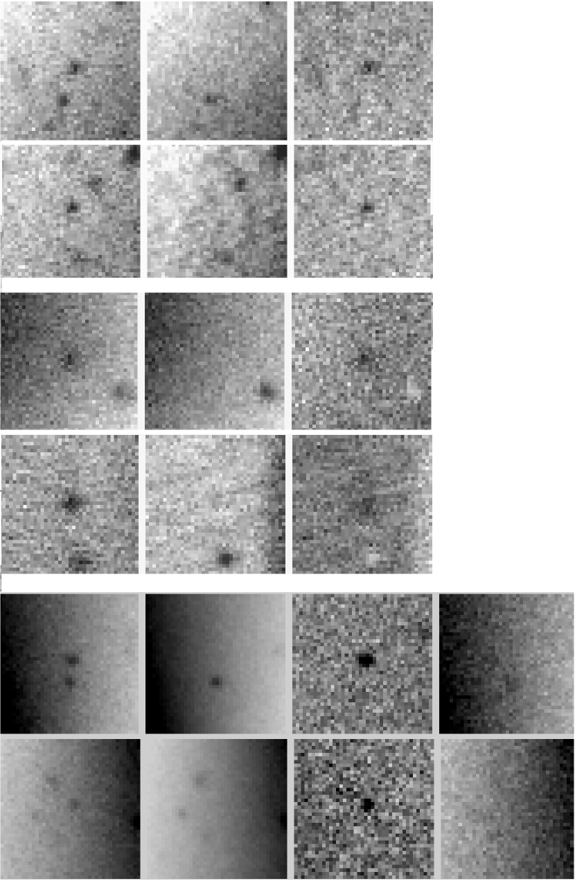
Figure 4.— Some examples of planetary nebula candidates in our target galaxies. From top to bottom, these candidates are from NGC 1316 (rows 1-2), NGC 1380 (rows 3-4), and NGC 4526 (rows 5-6). Column 1 (leftmost) shows a small region of the on-band image centered on each source, Column 2 shows the identical region in the off-band image, and Column 3 shows the difference of the on-band and off-band images. For NGC 4526, we have images in the H$\alpha$ band, and these are included in Column 4. For each galaxy, we present one PN candidate near the bright luminosity function cutoff (upper), and the other candidate near the adopted photometric completeness limit (lower). All of these candidates have stellar image profiles, are present in the on-band and difference images, but are completely absent in the off-band image, and are weak to nonexistent in the H$\alpha$ images, making them likely PN candidates.

Figure 5.— The planetary nebula luminosity functions for NGC 1316 and NGC 1380 binned into 0.2 mag intervals. The solid lines represent the empirical PNLF of equation (2) convolved with the mean photometric error vs. magnitude relation and translated to the most likely distance modulus for each galaxy. The solid circles represent objects in our statistical PN samples; the open circles indicate objects fainter than the completeness limit that were not included in the maximum likelihood solution.

Figure 6.— The planetary nebula luminosity functions for NGC 4526 binned into 0.2 mag intervals. The solid circles represent objects in the statistical PN sample; the open circles indicate objects fainter than the completeness limit that were not included in the maximum likelihood solution. Note the shallow drop-off in this PNLF compared to our other observations.

Figure 7.— The results from the maximum likelihood analysis for the PNLF of NGC 4526. The x-axis denotes the true distance modulus; the y-axis is the probability that the observed PNLF is drawn from the empirical model at the given distance. Corrections for extinction and photometric error have been applied. The solid line shows the function for the entire data sample, the long-dashed line shows the result for the 47 PN candidates in the outer sample, and the short-dashed line shows the results for the 47 PN candidates in the inner sample. There is a clear offset in the derived distance between the different samples.

Figure 8.— A direct comparison of the observed PNLFs of NGC 4526, and from the intracluster planetary nebulae field IPN 6, which is located $47{\tt{}^{\prime}}\mskip-6.0mu.\,5$ ($\approx$ 210 kpc) away from NGC 4526. As can be clearly seen, the brightest IPN have comparable magnitudes to the brightest PN candidates in NGC 4526.

Figure 9.— The completeness function for NGC 524 and NGC 1448 as a function of magnitude, with the error bars derived assuming the binomial distribution. The solid line is the best-fitting function of Fleming et al. (1995). In the case of NGC 524, the fit is excellent, but due to crowding, the original fit of NGC 1448 (given as the dashed line) is relatively poor. After re-fitting the function, omitting the points fainter than an instrumental magnitude of 28 which are effected by crowding, we obtain a much better fit (given as the solid line).

Figure 10.— The limits on the distance for NGC 524 and NGC 1448 as a function of expected number of objects. The thick solid line denotes the distance limit, while the vertical solid and dashed line show the 90% and 50% completeness levels from the artificial star experiments. The filled regions denotes where the distance limits are ruled out. Note the differences between the two curves, due to the differing completeness functions.

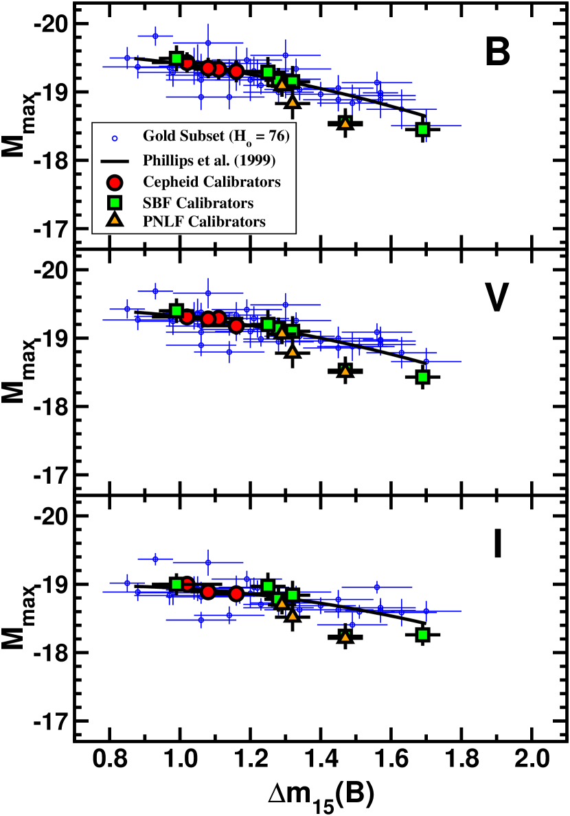
Figure 11.— The absolute magnitudes of SNe Ia at maximum light in the $B$, $V$, and $I$ bands, derived from the Cepheid, SBF, and PNLF distance indicators, and compared to the “gold” subset of Riess et al. (2004). The supernova maximum magnitude versus $\Delta m_{15}(B)$relation of Phillips et al. (1999) is overplotted for reference. The point at $\Delta m_{15}(B)$= 1.47 is SN 1992A, which is discussed in the text.

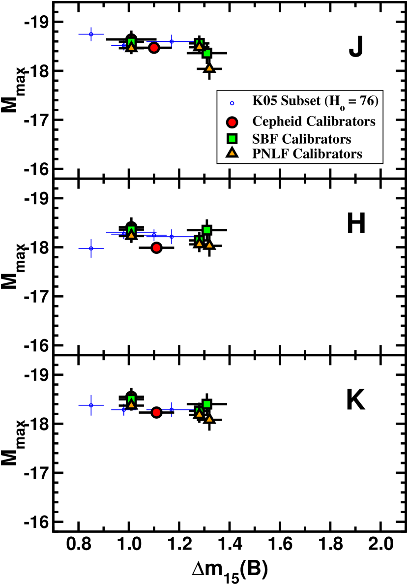
Figure 12.— The absolute magnitudes of SNe Ia at maximum light in the $J$, $H$, and $K$ bands, similar to Figure 11. Note the lack of a strong correlation with decline rate, as was originally found by Krisciunas, Phillips, & Suntzeff (2004).

References

- Aguerri et al. (2005) Aguerri, J. A. L., Gerhard, O. E., Arnaboldi, M., Napolitano, N. R., Castro-Rodriguez, N., & Freeman, K. C. 2005, AJ, 129, 2585
- Barbon et al. (1999) Barbon, R., Buondí, V., Cappellaro, E., & Turatto, M. 1999, A&AS, 139, 531
- Binggeli, Tammann & Sandage (1987) Binggeli, B., Tammann, G. A. & Sandage, A. 1987, AJ, 94, 251
- Boisseau & Wheeler (1991) Boisseau, J. R., & Wheeler, J. C. 1991, AJ, 101, 1281
- Busko (1996) Busko, I. C. 1996, ASP Conf. Ser. 101: Astronomical Data Analysis Software and Systems V, 5, 139
- Buzzoni (1989) Buzzoni, A. 1989, ApJS, 71, 817
- Cardelli, Clayton, & Mathis (1989) Cardelli, J.A., Clayton, G.C., & Mathis, J.S. 1989, ApJ, 345, 245
- Ciardullo et al. (1989) Ciardullo, R., Jacoby, G.H., Ford, H.C., & Neill, J.D. 1989, ApJ, 339, 53
- Ciardullo et al. (2002) Ciardullo, R., Feldmeier, J. J., Jacoby, G. H., Kuzio de Naray, R., Laychak, M. B., & Durrell, P. R. 2002, ApJ, 577, 31
- Ciardullo et al. (1994) Ciardullo, R., Jacoby, G., & Feldmeier, J. 1994, Bulletin of the American Astronomical Society, 26, 1400
- Ciardullo et al. (1998) Ciardullo, R., Jacoby, G. H., Feldmeier, J. J., & Bartlett, R. E. 1998, ApJ, 492, 62
- Ciardullo (1995) Ciardullo, R. 1995, in IAU Highlights of Astronomy, 10, ed. I. Appenzeller (Dordrecht: Kluwer), p. 507
- Ciardullo (2005) Ciardullo, R. 2005, AIP Conf. Proc. 804: Planetary Nebulae as Astronomical Tools, 804, 277
- de Vaucouleurs et al. (1991) de Vaucouleurs, G., de Vaucouleurs, A., Corwin, H. G., Buta, R.J., Fouqué, P., & Paturel, G. 1991, Third Reference Catalogue of Bright Galaxies, (New York: Springer-Verlag)
- Drenkhahn & Richtler (1999) Drenkhahn, G., & Richtler, T. 1999, A&A, 349, 877
- Feldmeier et al. (2003) Feldmeier, J. J., Ciardullo, R., Jacoby, G. H., & Durrell, P. R. 2003, ApJS, 145, 65
- Feldmeier et al. (2004) Feldmeier, J. J., Ciardullo, R., Jacoby, G. H., & Durrell, P. R. 2004, ApJ, 615, 196
- Feldmeier et al. (2002) Feldmeier, J. J., Mihos, J. C., Morrison, H. L., Rodney, S. A., & Harding, P. 2002, ApJ, 575, 779
- Filippenko (2005) Filippenko, A. V. 2005, White dwarfs: cosmological and galactic probes, 97
- Fleming et al. (1995) Fleming, D. E. B., Harris, W. E., Pritchet, C. J., & Hanes, D. A. 1995, AJ, 109, 1044
- Freedman et al. (2001) Freedman, W. L., et al. 2001, ApJ, 553, 47
- Freedman & Madore (1998) Freedman, W. L.& Madore, B. F. 1998, in Stellar Astrophysics for the Local Group, ed. A. Aparicio, A. Herrero, & F. Sańchez (New York: Cambridge Univ. Press), 263
- Gallagher et al. (2005) Gallagher, J. S., Garnavich, P. M., Berlind, P., Challis, P., Jha, S., & Kirshner, R. P. 2005, ApJ, 634, 210
- Gibson et al. (2000) Gibson, B. K., et al. 2000, ApJ, 529, 723
- Gibson & Stetson (2001) Gibson, B. K., & Stetson, P. B. 2001, ApJ, 547, L103
- Goudfrooij et al. (1994) Goudfrooij, P., de Jong, T., Hansen, L., & Norgaard-Nielsen, H. U. 1994, MNRAS, 271, 833
- Hamuy et al. (1995) Hamuy, M., Phillips, M. M., Maza, J., Suntzeff, N. B., Schommer, R. A., & Aviles, R. 1995, AJ, 109, 1
- Hamuy et al. (1996a) Hamuy, M., Phillips, M. M., Suntzeff, N. B., Schommer, R. A., Maza, J., & Aviles, R. 1996a, AJ, 112, 2391
- Hamuy et al. (1996b) Hamuy, M., Phillips, M. M., Suntzeff, N. B., Schommer, R. A., Maza, J., & Aviles, R. 1996b, AJ, 112, 2398
- Hamuy et al. (2000) Hamuy, M., Trager, S. C., Pinto, P. A., Phillips, M. M., Schommer, R. A., Ivanov, V., & Suntzeff, N. B. 2000, AJ, 120, 1479
- Harris (1990) Harris, W. E. 1990, PASP, 102, 949
- Hickey et al. (2004) Hickey, T., Gronwall, C., Ciardullo, R., Feldmeier, J., Gawiser, E., Herrera, D., & MUSYC 2004, Bulletin of the American Astronomical Society, 36, 1447
- Hoeflich et al. (1998) Hoeflich, P., Wheeler, J. C., & Thielemann, F. K. 1998, ApJ, 495, 617
- Howell et al. (2003) Howell, S. B., Everett, M. E., Tonry, J. L., Pickles, A., & Dain, C. 2003, PASP, 115, 1340
- Jacoby et al. (1990) Jacoby, G. H., Ciardullo, R., & Ford, H. C. 1990, ApJ, 356, 332
- Jacoby et al. (1992) Jacoby, G. H., et al. 1992, PASP, 104, 599
- Jacoby & Acker (2006) Jacoby, G. H., & Acker, A. 2006, in Planetary Nebulae in our Galaxy and Beyond - IAU Symposium 234
- Jedrzejewski (1987) Jedrzejewski, R. I. 1987, MNRAS, 226, 747
- Jensen et al. (2003) Jensen, J. B., Tonry, J. L., Barris, B. J., Thompson, R. I., Liu, M. C., Rieke, M. J., Ajhar, E. A., & Blakeslee, J. P. 2003, ApJ, 583, 712
- Jha et al. (1999) Jha, S., et al. 1999, ApJS, 125, 73
- Krisciunas et al. (2000) Krisciunas, K., Hastings, N. C., Loomis, K., McMillan, R., Rest, A., Riess, A. G., & Stubbs, C. 2000, ApJ, 539, 658
- Krisciunas et al. (2003) Krisciunas, K., et al. 2003, AJ, 125, 166
- Krisciunas, Phillips, & Suntzeff (2004) Krisciunas, K., Phillips, M. M., & Suntzeff, N. B. 2004, ApJ, 602, L81
- Krisciunas et al. (2006) Krisciunas, K., Prieto, J. L., Garnavich, P. M., Riley, J.-L. G., Rest, A., Stubbs, C., & McMillan, R. 2006, AJ, 131, 1639
- Li et al. (2001) Li, W., et al. 2001, PASP, 113, 1178
- Lira (1995) Lira, P. 1995, Masters thesis, Univ. of Chile
- Macri et al. (2001) Macri, L. M., Stetson, P. B., Bothun, G. D., Freedman, W. L., Garnavich, P. M., Jha, S., Madore, B. F., & Richmond, M. W. 2001, ApJ, 559, 243
- Massey et al. (1988) Massey, P., Strobel, K., Barnes, J. V., & Anderson, E. 1988, ApJ, 328, 315
- McMillan et al. (1993) McMillan, R., Ciardullo, R., & Jacoby, G. H. 1993 (MCJ1993), ApJ, 416, 62
- Monet (1998) Monet, D. 1998, BAAS, 30, 1427
- Monet et al. (1996) Monet, D., Bird, A., Canzian, B., Harris, H., Reid, N., Rhodes, A., Sell, S., Ables, H., Dahn, C., Guetter, H., Henden, A., Leggett, S., Levinson, H., Luginbuhl, C., Martini, J., Monet, A., Pier, J., Riepe, B., Stone, R., Vrba, F., & Walker, R. 1996, USNO A - 1.0 A catalog of astrometric standards, U.S. Naval Observatory, Washington, D. C.
- Nomoto et al. (1999) Nomoto, K. Umeda, H., Hachisu, I., Kato, M., Kobayashi, C. & Tsujimoto, T. 2000, in Type Ia Supernovae: Theory and Cosmology, ed. J.C. Niemeyer & J. W. Truran (Cambridge: Cambridge Univ. Press), 63
- Osip et al. (2004) Osip, D. J., et al. 2004, Proc. SPIE, 5492, 49
- Perlmutter et al. (1999) Perlmutter, S., et al. 1999, ApJ, 517, 565
- Phillips (1993) Phillips, M. M. 1993, ApJ, 413, L105
- Phillips et al. (1999) Phillips, M. M., Lira, P., Suntzeff, N. B., Schommer, R. A., Hamuy, M., & Maza, J. 1999, AJ, 118, 1766
- Pierce & Jacoby (1995) Pierce, M. J., & Jacoby, G. H. 1995, AJ, 110, 2885
- Prugniel & Heraudeau (1998) Prugniel, P., & Heraudeau, P. 1998, A&AS, 128, 299
- Richtler (2003) Richtler, T. 2003, Lecture Notes in Physics, Berlin Springer Verlag, 635, 281
- Riess, Press, & Kirshner (1996) Riess, A. G., Press, W. H., & Kirshner, R. P. 1996, ApJ, 473, 88
- Riess et al. (1998) Riess, A. G., et al. 1998, AJ, 116, 1009
- Riess et al. (2004) Riess, A. G., et al. 2004, ApJ, 607, 665
- Riess et al. (2005) Riess, A. G., et al. 2005, ApJ, 627, 579
- Rubin et al. (1999) Rubin, V. C., Waterman, A. H., & Kenney, J. D. P. 1999, AJ, 118, 236
- Saha et al. (2001) Saha, A., Sandage, A., Tammann, G. A., Dolphin, A. E., Christensen, J., Panagia, N., & Macchetto, F. D. 2001, ApJ, 562, 314
- Saha et al. (2006) Saha, A., Thim, F., Tammann, G. A., Reindl, B., & Sandage, A. 2006, ApJS, 165, 108
- Schlegel, Finkbeiner, & Davis (1998) Schlegel, D.J., Finkbeiner, D.P., & Davis, M. 1998, ApJ, 500, 525
- Spergel et al. (2006) Spergel, D. N., et al., ApJ, submitted - available as astro-ph/0603449
- Stetson (1987) Stetson, P. B. 1987, PASP, 99, 191
- Stone (1977) Stone, R.P.S. 1977, ApJ, 218, 767
- Stone & Baldwin (1983) Stone, R.P.S., & Baldwin, J.A. 1983, MNRAS, 204, 347
- Strolger & Riess (2006) Strolger, L.-G., & Riess, A. G. 2006, AJ, 131, 1629
- Sullivan et al. (2006) Sullivan, M., et al. 2006, ApJ, 648, 868
- Suntzeff et al. (1999) Suntzeff, N. B., et al. 1999, AJ, 117, 1175
- Tonry et al. (2001) Tonry, J. L., Dressler, A., Blakeslee, J. P., Ajhar, E. A., Fletcher, A. B., Luppino, G. A., Metzger, M. R., & Moore, C. B. 2001, ApJ, 546, 681
- Tonry et al. (2002) Tonry, J. L., Luppino, G. A., Kaiser, N., Burke, B. E., & Jacoby, G. H. 2002, Proc. SPIE, 4836, 206
- Umeda et al. (1999) Umeda, H., Nomoto, K., Kobayashi, C., Hachisu, I., & Kato, M. 1999, ApJ, 522, L43
- Valdes (2002) Valdes, F. 2002, in Automated Data Analysis in Astronomy, ed. R. Gupta, H. Singh, & C. A. L. Bailer-Jones (New Delhi, India: Narosa Publishing House), 309.
- Yungelson & Livio (2000) Yungelson, L. R., & Livio, M. 2000, ApJ, 528, 108