Insight into the baryon-gravity relation in galaxies

Abstract

Observations of spiral galaxies strongly support a one-to-one analytical relation between the inferred gravity of dark matter at any radius and the enclosed baryonic mass. It is baffling that baryons manage to settle the dark matter gravitational potential in such a precise way, leaving no “messy” fingerprints of the merging events and “gastrophysical” feedbacks expected in the history of a galaxy in a concordance Universe. This correlation of gravity with baryonic mass can be interpreted from several non-standard angles, especially as a modification of gravity called T$e$V$e$S, in which no galactic dark matter is needed. In this theory, the baryon-gravity relation is captured by the dieletric-like function $\mu$ of Modified Newtonian Dynamics (MOND), controlling the transition from $1/r^{2}$ attraction in the strong gravity regime to $1/r$ attraction in the weak regime. Here, we study this $\mu$-function in detail. We investigate the observational constraints upon it from fitting galaxy rotation curves, unveiling the degeneracy between the stellar mass-to-light ratio and the $\mu$-function as well as the importance of the sharpness of transition from the strong to weak gravity regimes. We also numerically address the effects of non-spherical baryon geometry in the framework of non-linear T$e$V$e$S, and exhaustively examine how the $\mu$-function connects with the free function of that theory. In that regard, we exhibit the subtle effects and wide implications of renormalizing the gravitational constant. We finally present a discontinuity-free transition between quasi-static galaxies and the evolving Universe for the free function of T$e$V$e$S, inevitably leading to a return to $1/r^{2}$ attraction at very low accelerations in isolated galaxies.

I Introduction

Data on large scale structures point towards a Universe dominated by dark matter (DM) and dark energy Spergel ; Clowe . Nowadays, the dominant paradigm is that DM is actually made of non-baryonic weakly-interacting massive particles, the so-called cold dark matter (CDM). However, on galaxy scales, the observations appear to be at variance with a sizeable list of CDM predictions. Measurements of non-circular motions in the Milky Way have shown that there is actually very little room for an axisymmetric distribution of dark matter inside the solar radius Bis03 ; FB05 , where CDM simulations predict a cuspy density profile Di . Even though CDM halos themselves could well be triaxial triax , the non-circular motion of gas in the inner Milky Way is proven to be linked with non-axisymmetric baryonic features such as the bar and the spiral arms Bis03 , thus leaving no room for a cuspy triaxial CDM halo to explain them. External galaxies have also been used to compare the predicted cuspy CDM density profiles with the observations, in particular rotation curves of dwarf and spiral galaxies. Despite the presence of observational systematic effects Swa , most of which are now under control, observations point towards dark matter halos with a central constant density core deblok ; Gen1 ; Gen2 ; Simon ; Kuzio at odds with the CDM predictions. Another interesting problem faced by CDM on galactic scales is the overabundance of predicted satellite galaxies compared to the observed number in Milky Way-sized galaxies Moore .

What is more, it is now well-documented that rotation curves suggest a correlation between the mass profiles of the baryonic matter (stars + gas) and dark matter Don ; McG ; McGa . Some rotation curves even display obvious features (bumps or wiggles) that are also clearly visible in the stellar or gas distribution Broeils . A solution to all these problems, and especially the baryon-DM relation, could be some kind of new specific interaction between baryons and some exotic DM McG . On the other hand, it could indicate that, on galaxy scales, the observed discrepancy rather reflects a breakdown of Newtonian dynamics in the ultra-weak field regime: this original proposal, dubbed MOND (Modified Newtonian Dynamics), was made more than twenty years ago in a series of hallmark papers Milgrom83 ; Milg2 ; Milg3 . But as noted in, e.g., Milgrom05 , a modified gravity theory is in many ways equivalent to an exact relation between baryons and dark matter. When analyzing rotation curves, the two interpretations are nearly degenerate in the sense that the fraction of gravity unaccounted by the Newtonian gravity of the baryons at radius $R$ is

$$1-\frac{\xi G_{N}M_{b}(R)}{R^{2}g}=\begin{cases}\frac{G_{N}M_{DM}(R)}{R^{2}g}&{\rm in}\,{\rm DM}\,{\rm picture}\cr\left[1-\mu(g/a_{0})\right]&{\rm in}\,{\rm MOND}\,{\rm picture}\cr\end{cases}$$ (1)

where $G_{N}$ is the usual Newtonian gravitational constant, $M_{b}(R)$ is the baryonic mass interior to the galactocentric radius $R$, $\frac{\xi G_{N}M_{b}(R)}{R^{2}}$ denotes the Newtonian gravity of the baryons (with a shape factor $\xi\sim 1$ to correct for non-spherical baryon distribution), and $g=v^{2}/R$ is the total centripetal gravitational acceleration from measuring the circular speed $v$ at radius $R$. The first equality introduces a spherical halo of dark matter with mass $M_{\rm DM}(R)$ enclosed inside radius $R$ (a flattening factor can also be used for the DM halo). The second equality (Milgrom’s law) invokes a modified dynamics with a dielectric-like Blanchet1 ; Blanchet2 factor $\mu\leq 1$ to boost Newtonian gravity below a dividing acceleration scale $a_{0}$ whose value turns out to be of the same order as $cH_{0}$. This $\mu$ factor is also called the MOND interpolating function $\mu(x)$ (where $x=g/a_{0}$).

The key difference between the usual dark matter and the MOND interpretation is the fact that MOND requires all galaxies to share the same $\mu$-function for the same value of $a_{0}$. If it is not the case, then the present-day success of MOND just tells us something phenomenological about DM. On the other hand, if it is indeed exactly the case, then either a to-be-discovered exotic relation does actually exist between DM (not the usual CDM) and baryons, or the DM paradigm is incorrect on galaxy scales. In the latter case, either gravity should be modified BM84 ; Bekenstein2004 , which could lead to some subtle differences regarding e.g. dynamical friction dynf1 ; dynf or tides Zglob ; ZT , or inertia should be modified Milgrom05 ; Milgrom94 ; Milgrom99 , which would lead to very significant differences with the DM interpretation, especially in non-stationary situations Milgrom05 .

The basis of the MOND paradigm Milgrom83 is that $\mu$ is a function which runs smoothly from $\mu(x)=1$ at $x\gg 1$ to $\mu(x)=x$ at $x\ll 1$. Even though this leaves some freedom for the exact shape of $\mu$, it is already extremely surprising, from the DM point of view, that such a prescription did predict many aspects of the dynamics of galaxies such as the appearance of large discrepancies with Newtonian dynamics in low surface brightness galaxies, as well as the absence of discrepancies in the inner parts of high surface brightness ones. With this definition of the $\mu$-function, the fraction of gravity unaccounted by Newtonian gravity tends to zero in the high-acceleration limit, and one recovers in the low-acceleration limit the Tully-Fisher law Tully ; McG2 , which tells us that the circular velocity at the last measured radius in spiral galaxies must behave like $M_{b}^{1/4}$. Since the centripetal acceleration at that radius is typically lower than $\sim 0.4a_{0}$ in high surface brightness galaxies (and even lower in low surface brightness galaxies), the MOND circular velocity at that radius is within at most ten percent of the asymptotic one, depending on the exact shape of the $\mu$-function, and on the stellar mass-to-light ratio. Indeed, the exact shape of the $\mu$-function is still somewhat ambiguous in MOND, because there is a degeneracy between the choice of $\mu$ and the stellar mass-to-light ratio when rotation curves are fitted with Eq. (1). While the exact asymptotic velocity will actually be different depending on the mass-to-light ratio, the shape of the $\mu$-function will at the same time determine at what radius the rotation curve really becomes flat, and this can happen somewhat away from the last observed radius, thus explaining this degeneracy.

Even though the most important aspect of MOND, confronting CDM with the most severe observational difficulties, remains its asymptotic behaviour described above, the study of the transition between the Newtonian regime and the asymptotic MOND regime, characterized by the shape of the $\mu$-function, may also be important in the quest for a possible fundamental theory underpinning the MOND prescription. In this contribution, we thus investigate the observational constraints upon the $\mu$-function in that transition zone, as well as the theoretical constraints upon it in the framework of Bekenstein’s relativistic multifield theory of gravity Bekenstein2004 .

II Observational constraints on the $\mu$-function

II.1 The $\alpha$-family and the standard function

In this section, we examine the observational constraints upon the $\mu$-function from fitting galaxy rotation curves with Milgrom’s law (the second equality of Eq. 1). As a matter of fact, we shall prove in Sect. III F that this empirical law yields an excellent approximation to Bekenstein’s relativistic multifield theory of MOND Bekenstein2004 in fitting rotation curves of spiral galaxies.

Here, we explicitly show the degeneracy between the stellar mass-to-light ratio (+ the distance of the galaxy) and the shape of the $\mu$-function, a degeneracy that prevents from fixing the $\mu$-function in present-day MOND. Among a parametric family of $\mu$-functions, we are going to show that the best fits are obtained for the “simple” $\mu$-function of FB05 :

$$\mu(x)=\frac{x}{1+x},$$ (2)

and that, notwithstanding the $M_{*}/L$-$\mu$ degeneracy (where $M_{*}/L$ is the stellar mass-to-light ratio), $\mu$-functions with too slow a transition from the Newtonian to the deep-MOND regime are excluded by rotation curves data, while the “standard” $\mu$-function SanMc ,

$$\mu(x)=\frac{x}{\sqrt{1+x^{2}}},$$ (3)

with a faster transition than Eq. (2), yield fits of comparable quality.

The set of $\mu$-functions we propose to test against observations is called the $\alpha$-family AFZ :

$$\mu(x)=\frac{2x}{1+(2-\alpha)x+\sqrt{(1-\alpha x)^{2}+4x}},~{}0\leq\alpha\leq 1.$$ (4)

In the $\alpha=1$ case, one directly recovers the simple function of Eq. (2). In the $\alpha=0$ case, it is a simple exercise to show that one recovers the $\mu$-function of Bekenstein’s toy-model (Bekenstein2004, , eq.(62))

$$\mu(x)=\frac{-1+\sqrt{1+4x}}{1+\sqrt{1+4x}}.$$ (5)

Figure 1: The $\mu$-functions of Eq. (4) for $\alpha=0$, $\alpha=0.5$, $\alpha=0.9$, and $\alpha=1$, illsutrating that the transition from the deep-MOND ($\mu\sim x$) to the Newtonian ($\mu\sim 1$) regime is sharper with increasing $\alpha$.

Fig. 1 displays those $\mu$ as a function of $x$. This is of course far from testing all the other possibilities, notably the free function proposed in sanderssolar , but it will give a good indication of the range of allowed $\mu$-functions to be compatible with observed rotation curves.

II.2 Fitting galaxy rotation curves

In order to test observationally the parametric $\alpha$-family of $\mu$-functions, we selected a sample made of two subsamples of rotation curves: the first subsample is made of nine rotation curves presented in BBS . This sample has been used to determine the value of the acceleration constant $a_{0}=1.21\times 10^{-8}$ cm s^-2 that is generally used in MOND studies with the standard $\mu$-function. The second subsample consists of the five galaxies presented in Gen1 . This way, we have a final sample of 14 galaxies with high-quality, extended rotation curves. These galaxies span a large range of Hubble types and maximal velocities, from small irregular dwarf galaxies to large early-type spirals.

The values of $a_{0}$ and $\alpha$ are unknown a priori, but have to be the same for all the galaxies. Therefore, we performed a global fit for these two parameters to the abovementioned 14 rotation curves: $\alpha$ was allowed to vary from $0$ to $1$, while the stellar $M/L$ ratio and the distance ($\pm 30\%$ the distances adopted in BBS and Gen1 ) were left as parameters free to vary individually for each galaxy (see Table I).

Table 1: Best-fit distances ($d$ in Mpc) and stellar $M/L$ ratios (in solar units) of the MOND rotation curve fits with the standard $\mu$-function (Eq. 3) and the simple $\mu$-function (Eq. 2, $\alpha=1$). Distances were left as free parameters within 30% of the distances adopted in the original papers; for NGC 7331 the bulge $M/L$ was considered as an additional free parameter, with a best-fit value of 1.5 for both $\mu$-functions. The degeneracy between those free parameters and the choice of the $\mu$-function appears clearly ($M_{*}/L$ playing the most important role in this regard).

Standard $\mu$

Simple $\mu$

Galaxy	$d$	$M_{*}/L$	$d$	$M_{*}/L$
NGC 2403	3.5	1.2	3.3	0.9
NGC 2903	6.5	3.5	5.1	3.4
NGC 3198	7.2	4.1	7.1	2.9
NGC 6503	5.5	2.0	5.5	1.4
NGC 7331	13.3	5.0	13.6	2.4
NGC 1560	3.4	0.4	3.0	0.4
NGC 2259	9.5	2.3	9.4	1.6
DDO 154	3.4	0.1	3.0	0.1
DDO 170	14.0	0.7	12.7	0.7
ESO 116-G12	20.0	0.3	19.8	0.2
ESO 287-G13	34.8	1.4	31.1	1.1
ESO 79-G14	28.1	2.1	25.6	1.7
NGC 1090	25.5	2.3	25.5	1.5
NGC 7339	23.4	1.4	23.4	0.9

The best fits are obtained for

$$\alpha=1^{+0.0}_{-0.5},$$ (6)

and

$$a_{0}=1.35^{+0.28}_{-0.42}\times 10^{-8}{\rm cm}\,{\rm s}^{-2},$$ (7)

where the errors are the one-sigma uncertainties from the $\chi^{2}$ statistics of the global fit; this value of $a_{0}$ is compatible with the result of BBS . For the unfavoured functions with $\alpha<0.5$, the transition from the deep-MOND to the Newtonian regime is slower than for $\alpha>0.5$ as shown on Fig. 1.

The results of the rotation curve fits using the best fit parameters $\alpha=1$ and $a_{0}=1.35\times 10^{-8}$ cm s^-2 are shown in Fig. 2. When comparing the fits of Fig. 2 to those performed with the standard MOND $\mu$-function (Eq.3, Fig. 3), we see that the simple $\mu$-function clearly fits the rotation curves as well as the standard one: the $\chi^{2}$ values of the fits are very similar. On average, we have:

$$\chi^{2}_{\alpha=1}/\chi^{2}_{standard}=0.98\pm 0.24.$$ (8)

Note however that three galaxies (NGC 2403, NGC 3198, and NGC 7331) also have Cepheid-based distances Bottema . While for NGC 2403 and NGC 7331 the best-fit distances (of both $\mu$-functions) are within 10% of the Cepheid distances, the best-fit distance of NGC 3198 is about a factor 2 smaller than the Cepheid-based one. Imposing this value of the distance slightly decreases the best-fit value of $a_{0}$ but it doesn’t change the best-fit value of $\alpha$, nor does it change significantly the result of Eq. (8), because the fits with both $\mu$ functions get worse for NGC 3198.

The relatively large error bars on $\alpha$ are due to the degeneracy between the shape of $\mu$ and the stellar $M/L$ ratio. Still, it is striking that, notwithstanding this degeneracy, $\alpha=1$, corresponding to the simple relation of Eq. (2), actually yields the best fit. This function was also shown to yield an excellent fit to the Terminal Velocity Curve of the Milky Way Galaxy FB05 , and was found to work better than the standard function to fit the dispersion profile of the globular cluster system of NGC 4636 in the transition regime between the Newtonian and the deep-MOND regime Schu . Even more interesting is to check that the stellar $M/L$ ratios implied by this simple $\mu$-function are realistic. On average, we have:

$$\frac{(M_{*}/L)_{\alpha=1}}{(M_{*}/L)_{\rm standard}}=0.70\pm 0.15.$$ (9)

i.e. their value is $\sim$30% lower than when using the standard MOND interpolating function. In McG the standard MOND $M/L$ ratios are slightly higher than the predictions of stellar population synthesis models (by $\sim$ 0.10 dex, using his fits of the stellar $M/L$ vs colour plots for B-V$>$0.55, i.e. above the break), for a given observed colour. Recently, dB compared the ranges of $M/L$ ratios allowed by different methods to determine them, and suggested that the normalisation of the stellar $M/L$ vs colour relation should be lowered by 0.05 to 0.10 dex. Note that they consider the predictions of the models by Bd , while McG uses the most recent models by bell . However, in the range of colours considered by McG , 0.4 $\lesssim$ B-V $\lesssim$ 0.8, the two models give predictions that differ by at most 0.03 dex. The stellar $M/L$ ratios that we find from the simple $\mu$-function, $\sim 30\%$ lower than the standard MOND ones, fall perfectly in this range allowed by the various constraints considered by dB .

Let us end this section by noting that the “traditional” view on this observational baryon-gravity relation would be that it is a purely empirical relation that will be understood within the framework of the concordance $\Lambda$CDM cosmological model. Even though this is a very challenging task, the meaning of the $\alpha$-family of Eq. (4) combined with Eq. (1) would then correspond (in spherical symmetry) to the following empirical relation:

$$\frac{g_{Nb}}{g_{DM}}=\frac{\alpha g_{Nb}+g_{DM}}{a_{0}},$$ (10)

where $g_{Nb}$ and $g_{DM}$ are the contribution to the rotation curve gravity from the baryons and DM respectively. If neither gravity nor inertia are to be modified, the present success of the simple relation $\alpha=1$ to fit galaxy rotation curves still captures the essence of the fine-tuning problem for dark matter. The mass-to-light ratios of Table I being compatible with current population synthesis models, Eq. (10) tells us that the ratio of baryonic gravity to DM gravity should be equal to the total gravity in units of $a_{0}$. For example, if one plots the contribution of baryons and dark matter to the rotation curve at a certain radius as a function of the baryonic contribution to gravity at that radius (Fig. 4), one finds a cross reminiscent of McG .

Figure 2: Rotation curve decompositions with $\alpha=1$ [see Eq.(4) and Eq.(2)] and $a_{0}=1.35\times 10^{-8}$ cm s^-2. The distances were left as free parameters, within 30% of the adopted distances in the original papers. The solid line is the best fit to the data, the dotted/dashed/long-dashed lines represent the disk/gas/bulge Newtonian contributions. Note that the Newtonian curves deviate from the MOND ones even at small radii, which is characteristic of the simple function $\alpha=1$.

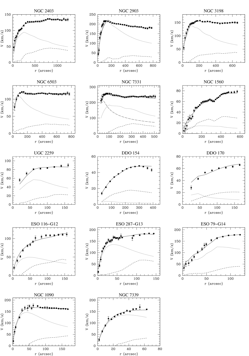
Figure 3: Rotation curve decompositions with the standard MOND $\mu$-function [see Eq.(3)], and $a_{0}=1.21\times 10^{-8}$ cm s^-2. The distances were left as free parameters, within 30% of the adopted distances in the original papers. The solid line is the best fit to the data, the dotted/dashed/long-dashed lines represent the disk/gas/bulge Newtonian contributions. Note that the distances were already allowed to vary in fits with the standard function in BBS (and that the fits presented on this figure are thus the same) but not in Gen1 .

Figure 4: This figure illustrates that Eq. (10) captures the essence of the fine-tuning problem for CDM in galaxies. For $\alpha=1$, we plot the square root of the fraction of total gravity accounted by the baryons (dashed line) and the DM (full line) as a function of the logarithm of baryonic gravity. The cross is reminiscent of the one obtained in (McG, , fig.4).

III The $\mu$-function and the free function of T$e$V$e$S

III.1 T$e$V$e$S in galaxies

Here, we present the theoretical constraints upon the $\mu$-function in the framework of Bekenstein’s relativistic multifield theory of gravity Bekenstein2004 . Before doing that, we need to briefly look back on the basics of the theory, and recap the relevant equations (in Sects. III A and III B).

If one wants to modify Newtonian gravity on galaxy scales in order to get MOND, one can modify Poisson’s equation in order to recover Milgrom’s law (second equality in Eq. 1) in highly symmetric systems BM84 , namely:

$$\nabla.[\mu(|{\bf\nabla}\Phi|/a_{0})\nabla\Phi]=4\pi G_{N}\rho,$$ (11)

where $G_{N}$ is the usual Newtonian gravitational constant, $\Phi$ is the MOND gravitational potential and $\rho$ is the density of the (baryonic) matter distribution. In spherical symmetry, one then immediately finds back Milgrom’s law (Eq. 1) from Gauss’s theorem. Out of spherical symmetry, one finds that

$$\mu(|{\bf\nabla}\Phi|/a_{0})\nabla\Phi=\nabla\Phi_{N}+\nabla\times{\bf h},$$ (12)

where ${\bf h}$ is a regular vector field determined (up to a gradient) by the condition that the curl of the total force $\nabla\Phi$ must vanish. Inside spiral galaxies, a numerical MOND potential solver Brada1 ; CLN ; Tiret must thus be used to obtain the exact MONDian force field corresponding to Eq. (11). However, it has been shown that Milgrom’s law is still a good enough approximation to fit galactic rotation curves within that framework Brada1 ; Brada2 .

On the other hand, the extension of General Relativity that has been proposed by Bekenstein for the MOND paradigm is a bi-metric multi-field theory Bekenstein2004 , namely a tensor-vector-scalar (T$e$V$e$S) theory leading to Milgrom’s law in spherical symmetry as we shall see below, but different from Eq. (11) in more general geometries AFZ . Interestingly, this theory can be reformulated in various fashions, such as e.g. a pure tensor-vector theory in the matter frame Zlosnik . We however concentrate here on the original formulation of the theory.

The tensor of the theory is the Einstein metric $g_{\alpha\beta}$ out of which is built the usual Einstein-Hilbert action, while the MONDian dynamics comes from a dynamical scalar field $\phi$ whose lagrangian density is aquadratic. All the matter fields are coupled to a physical metric involving the tensor and the scalar field of the theory (Bekenstein2004, , eq.(21)), and which must be disformally related to the Einstein metric in order to consistently enhance the deflection of photons. This needs the introduction of a dynamical normalized vector field $U_{\alpha}$. The total action is thus the sum of the Einstein-Hilbert action for the Einstein metric, the action of the scalar field, the action of the vector field, and the matter action involving the physical metric. Einstein-like equations are then obtained for each of these fields by varying the action w.r.t. each of them Bekenstein2004 .

The action of the scalar field $\phi$ can be written

$$S_{s}=-\frac{1}{2k^{2}l^{2}G}\int{\rm d}^{4}x\sqrt{-g}f(y)$$ (13)

where $G$ is the bare gravitational constant appearing in the Einstein-Hilbert action, $g$ is the determinant of the Einstein metric, and $y=c^{-4}kl^{2}h^{\alpha\beta}\partial_{\alpha}\phi\partial_{\beta}\phi$ (the metric $h^{\alpha\beta}$ being some specific combination of the Einstein metric and the vector field Bekenstein2004 ). Here $k$ is a small dimensionless parameter (of the order of one percent) determining the strength of the scalar coupling to matter, $l$ is a length scale linked to the acceleration scale $a_{0}$, and $c$ is the speed of light. The function $f(y)$ is a free function driving the dynamics of the scalar field, that can be identified (to a factor) with its lagrangian density , and that yields the MOND behaviour in galaxies when judiciously chosen. Note that for quasi-static systems (for which time derivatives are zero) such as galaxies, the scalar field is akin to k-essence scalar fields, that were notably introduced as possible dark energy fluids that could also drive inflation Damour ; Chiba ; Stein . This name comes from the fact that their dynamics is dominated by their kinetic term $-f(y)$, contrary to other quintessence models in which the scalar field potential plays the crucial role.

In the Einstein frame, matter fields couple to the three gravitational fields (tensor, vector and scalar field) through an effective “disformal” metric that differs from the Einstein metric, and which therefore, although dynamical, assumes a prior geometric form. In that frame the above k-essence field may thus be considered to mediate a “fifth force” ${\bf g}_{s}=-\nabla\phi$, in addition to the usual gravity connected to the gravitational tensor. On the other hand, shifting our viewpoint from the Einstein frame to the matter one, matter fields appear to couple to some metric that assumes no prior form, but which is determined by a non-diagonal system of coupled differential equations. In that case the scalar field does not trivially manifest as a fifth force. Those two points of view are however equivalent, and we shall now work in the Einstein frame.

If one couples such a k-essence field to the matter sector in the way it is done in T$e$V$e$S, one finds in the non-relativistic limit, neglecting pressure, and in a static configuration, the following modified Poisson’s equation (Bekenstein2004, , eq.(42)):

$${\bf\nabla}.\left[\nabla\phi f^{\prime}\left(c^{-4}kl^{2}|{\bf\nabla}\phi|^{2}\right)\right]=kG\rho,$$ (14)

where $\rho$ is the density of the matter distribution Bekenstein2004 . The analogy with Eq. (11) is striking. For a spherical distribution of mass $M$ one thus gets

$$\nabla\phi f^{\prime}(c^{-4}kl^{2}|{\bf\nabla}\phi|^{2})=\frac{kGM{\bf r}}{r^{3}}$$ (15)

outside the matter. It must be stressed that many papers achieve to find modified theories of gravity in which a test particle has an asymptotic circular velocity of the form $v=\gamma c$ where $\gamma$ is a pure number of the theory, and thus seem to recover flat rotation curves of spiral galaxies Cadoni ; Sobouti ; Capo . However one must not only be concerned with the existence of the plateau velocity, but also with the whole phenomenology of rotation curves (see Sect. II and e.g. Pers ; GeSa ), including the Tully-Fisher relation Tully ; McG2 . This relation teaches us that $\gamma$ should behave as $M^{1/4}$ (at roughly a ten percent level due to the possible difference between the asymptotic velocity and the velocity at the last observed radius). In these theories it is not correct to set by hands such a value for $\gamma$. On the contrary, k-essence theories achieve this in a very elegant manner. It is indeed immediate to see that if $f^{\prime}(y)$ behaves as $\sqrt{y}$, then the “fifth force” dominates the Newton-Einstein gravity in the ultra-weak field limit, and both the asymptotic plateau velocity and its amplitude are recovered. K-essence theories would not have been useful if, say, the Tully-Fisher relation were $v^{p}\propto M$ with $p\neq 4$. In other words, k-essence theories are relevant toy-models in this context because the effective (MOND) gravitational field in the outskirts of galaxies is the square root of the Newtonian one.

III.2 T$e$V$e$S and Milgrom’s law

To the leading order, the physical metric near a quasi-static galaxy in T$e$V$e$S is given by the same metric as in General Relativity, with the standard Schwarzschild potential replaced by the total potential

$$\Phi=\Xi\phi_{n}+\phi\,,$$ (16)

where $\phi_{n}$ is the Newtonian potential obtained from using the bare gravitational constant $G$, and $\Xi\sim 1$ is a dimensionless parameter which slowly evolves with the cosmic time (Bekenstein2004, , eq.(58)). Note that this parameter can always be chosen to be precisely $\Xi=1$ at the present time. This means that, locally and at the classical level, the scalar field $\phi$ plays exactly the role of the dark matter potential. To the leading order, we have the following field equations in a quasi-static system:

$${\bf\nabla}^{2}\phi_{n}=4\pi G\rho,$$ (17)

i.e. the Poisson equation for the Newtonian potential, and

$${\bf\nabla}.[\mu_{s}(|{\bf\nabla}\phi|/a_{0}){\bf\nabla}\phi]=4\pi G\rho,$$ (18)

i.e. a MOND-like equation (see Eq. 11) for the scalar field, obtained from Eq. (14) by defining (noticing that $y>0$ in a static configuration)

$$\mu_{s}[(c^{2}/la_{0})\sqrt{y/k}]\equiv 4\pi f^{\prime}(y)/k.$$ (19)

Note that the acceleration scale $a_{0}$ does not need to be precisely constant through cosmic time. However, since the variation is extremely slow, it can be considered as effectively constant during the entire time that galaxies have existed (see Sect. III C). From Eqs. (16), (17), and (18) we are now able to look for a Milgrom’s law for the total gravitational potential $\Phi$. Note that we restrict ourselves to spherical symmetry so that we look for an equation of the form

$$\mu(|{\bf\nabla}\Phi|/a_{0})\nabla\Phi=\frac{G_{N}M(r){\bf r}}{r^{3}},$$ (20)

together with the usual asymptotic MONDian conditions $\mu(x)\sim x$ if $x\ll 1$ and $\mu(x)\sim 1$ if $x\gg 1$. The above equation notably implies that $G_{N}$ is the gravitational constant measured in Newtonian systems (and hence on Earth), which is not required to be equal to the bare one.

For commodity we define

$${\bf x}=-\frac{\nabla\Phi}{a_{0}}=\frac{{\bf g}}{a_{0}},~{}x=\frac{|{\bf\nabla}\Phi|}{a_{0}}=\frac{g}{a_{0}}$$ (21)

the MONDian gravitational force per unit mass and its modulus in units of $a_{0}$, and

$${\bf s}=-\frac{\nabla\phi}{a_{0}}=\frac{{\bf g}_{s}}{a_{0}},~{}s=\frac{|{\bf\nabla}\phi|}{a_{0}}=\frac{g_{s}}{a_{0}}$$ (22)

the scalar field force and its modulus in units of $a_{0}$. Given that $a_{0}$ can slowly (even though not much) vary with cosmic time , the very definition of $s$ slowly varies too.

In spherical symmetry, we thus have

$$\mu_{s}(s)s=\frac{1}{\Xi}(x-s)=\frac{|{\bf\nabla}\phi_{n}|}{a_{0}}.$$ (23)

Let us emphasize that the $\mu_{s}$ function can be quite arbitrarily chosen in a k-essence theory (but see Sect. IV.1), so that the $\mu$-function that will be derived from it may not possess the right MONDian behaviour. We shall therefore adopt a phenomenological point of view herafter, by imposing the standard asymptotic conditions for $\mu$, and look for the corresponding properties of $\mu_{s}$.

Let us define a parameter $\nu_{0}$ that connects the renormalized gravitational constant measured on Earth to its bare value: $G_{N}=\nu_{0}G$. In spherically symmetric T$e$V$e$S, Milgrom’s law can then be written as

$$\mu(x)x=\frac{\nu_{0}}{\Xi}(x-s),$$ (24)

meaning that the $\mu$-function is defined by

$$\mu\equiv\frac{\nu_{0}\mu_{s}}{1+\Xi\mu_{s}}.$$ (25)

Note that in (Bekenstein2004, , sect.IV B) Milgrom’s function was defined by

$${\tilde{\mu}}(x)x\equiv\frac{|{\bf\nabla}\phi_{n}|}{a_{0}},$$ (26)

neglecting the renormalization of $G$ as a first order approximation. Since it is always possible to immediately renormalize $G$ by a factor $\Xi$ such that the total potential in Eq. (16) is the sum of the Newtonian potential and the scalar field, it is tempting to define $\mu=\Xi{\tilde{\mu}}$. However, as we shall show hereafter, this renormalization is only valid for some special forms of the T$e$V$e$S free function. More generally the exact $\mu$-function of Eq. (25) is related to the one of Eq. (26) by $\mu=\nu_{0}{\tilde{\mu}}$, and the fact that $\nu_{0}$ may differ from $\Xi$ has wide implications.

In the rest of this section, we exhaustively examine how the free function of T$e$V$e$S, hereafter $\mu_{s}(s)$ as defined in Eq. (19), connects with the $\mu$-function of MOND, and we insist on the importance of this famous value of $\nu_{0}$ inherited from the shape of $\mu_{s}$.

III.3 The deep-MOND regime

In the deep-MOND regime, we must have $\mu(x)\sim x$ for $x\ll 1$, which implies, from Eq. (24), that $s\ll 1$ ($s\sim x$) and from Eq. (23) that

$$\mu_{s}(s)\sim\frac{s}{\nu_{0}}$$ (27)

in this regime. In order to get this behaviour in Eq. (19) with the standard choice $f^{\prime}(y)\sim\sqrt{y/3}$ for small $y$ Bekenstein2004 , we must define for the length scale:

$$l\equiv\frac{c^{2}\sqrt{3k}}{4\pi\nu_{0}a_{0}}.$$ (28)

Note that since $l$ is a parameter of the theory (fixed by definition), the above equation shows that $\nu_{0}a_{0}$ must be a constant. As we will see below however, the renormalization of $G$, encoded in the parameter $\nu_{0}$ depends on the cosmic time, since $\nu_{0}$ is related to $\Xi$. This implies that the acceleration scale $a_{0}$ does vary with cosmic time ($a_{0}$ is higher at higher redshift). Let us underline that what we call $a_{0}$ is the quantity determining the MONDian asymptotic circular velocity for a spherical system, since in the deep-MOND regime test-particles feel a force given by $\sqrt{GM\nu_{0}a_{0}}/r$ by virtue of Eqs. (23), (24) and (27). This force is interpreted by an observer on Earth as a force given by $\sqrt{G_{N}Ma_{0}}/r$, where $G_{N}=\nu_{0}G$ is our local constant of gravity. However Bekenstein Bekenstein2004 estimated that the time variation of $\Xi$ is extremely mild in the matter dominated period, so that as far as fits of galaxy rotation curves are concerned, this variation of $a_{0}$ is expected to have a negligible influence, even though $a_{0}$ is expected to be somewhat different at the epoch of nucleosynthesis.

Note also that Eq. (28) agrees with (Bekenstein2004, , eq.(62)) only in the very special case where $\nu_{0}=\Xi$. This special case is also very important in the study of the Newtonian regime, as we shall see hereafter.

III.4 The Newtonian regime: unbounded $\mu_{s}$-function

The case $\nu_{0}=\Xi$ is a physically interesting one, because, a priori, it is always possible to immediately renormalize $G$ in Eq. (17), such that $\Xi\phi_{n}=\Phi_{N}$. Then, also replacing $G$ by $G_{N}=\Xi G$ in the scalar field modified Poisson equation (Eq. 18) means that the phenomenologically relevant interpolating function for the scalar field becomes $\Xi\mu_{s}$ (during a period for which the parameter $\Xi$ is constant, which is effectively the case during the entire time that galaxies have existed), and that the particular case $\nu_{0}=\Xi$ thus corresponds to no a posteriori renormalization of the gravitational constant. Eq. 23) and Eq. (24) can then be rewritten:

$$x-s=\mu(x)x=\Xi\mu_{s}(s)s$$ (29)

The question is then whether it is actually $possible$ to have $\nu_{0}=\Xi$. Let us first show that we indeed have $\nu_{0}=\Xi$ if and only if the $\mu_{s}$-function is unbounded, i.e. $\mu_{s}\rightarrow\infty$. Indeed, if $\nu_{0}=\Xi$, then, from the first equality in Eq. (29), we can write $\mu$ as $1-s/x$ where we must have $s\ll x$ for the Newtonian regime $x\gg 1$, which proves from the second equality in Eq. (29) $s=x/(1+\Xi\mu_{s})$ that $\mu_{s}$ must diverge with $s$. Respectively, if $\mu_{s}(s)$ diverges for some value $s=s_{0}$, it is straightforward from Eq. (25) that $\mu\rightarrow\nu_{0}/\Xi$ and therefore that $\nu_{0}=\Xi$ by definition of $\mu$.

Then let us emphasize that Eq. (29) actually corresponds to the implicit assumptions in ZF06 , where it was shown that, without any a posteriori renormalization of the gravitational constant, it was impossible to find a T$e$V$e$S free function $\mu_{s}(s)$ corresponding to the standard $\mu$-function of MOND (Eq. 3). This particular result can actually be generalized through the following theorem:

When $\nu_{0}=\Xi$, a MOND $\mu$-function can be obtained from a T$e$V$e$S free function only if $n\leq 1$ in its asymptotic expansion $\mu(x)\sim 1-A/x^{n}$ (where $A$ is some positive constant).

The proof is quite straightforward:

Since $\nu_{0}=\Xi$, we have from Eq. (24) (or from the first equality in Eq. 29)

$$s=x[1-\mu(x)]\,.$$ (30)

Let us assume that $n>1$, then for $x\rightarrow\infty$ we would have $s\sim A/x^{n-1}\rightarrow 0$. But since $s\ll 1$ is already the deep-MOND regime (see Sect. III C), it cannot be also the Newtonian one $\square$

What it means is that, as can be easily checked ZF06 , the $\mu_{s}$ function would be multivalued. This is however not acceptable since $\mu_{s}$ must define unambiguously the dynamics of the scalar field. No unbounded $\mu_{s}$-function can thus reproduce the standard $\mu$-function (Eq. 3), for the reason that the latter admits the following asymptotic expansion

$$\mu(x)\sim 1-\frac{1}{2x^{2}},$$ (31)

and by virtue of the previous theorem (here $n=2$).

On the other hand, if $n<1$, this is not a problem since $s$ would diverge jointly with $x$, while if $n=1$, $s$ would asymptote to a finite positive value, and the function $s(x)$ from Eq. (30) could still be strictly increasing, and thus be invertible. E.g., the simple $\mu$-function of MOND, (Eq. 2), has $n=1$ for its asymptotic expansion. Its corresponding function $s(x)$ from Eq. (30) is

$$s(x)=\frac{x}{1+x},$$ (32)

leading to the unbounded $\mu_{s}$ function

$$\Xi\mu_{s}(s)=\frac{s}{1-s}.$$ (33)

This corresponds to the $n=0$ case of the free function proposed by (ZF06, , eq.(13)) for the local value $\Xi=1$. The $\mu$-functions tested against observations in Sect. II also have an unbounded $\mu_{s}$ counterpart in T$e$V$e$S. If we want their corresponding k-essence free functions to be expressed as pure functions of the constants in the action of T$e$V$e$S (see Sect. III A), independently of cosmic variations of $\Xi$, we can write the $\alpha$-family of Eq. (4) as:

$$\mu_{s}(s)=\frac{s}{\Xi-\alpha s}.$$ (34)

Another interesting aspect of these unbounded $\mu_{s}$ functions (or of the special case $\nu_{0}=\Xi$) is that they lead to an analogy with electromagnetism that might be helpful to grasp the feeling of the to-be-understood physical meaning of the scalar field of T$e$V$e$S. Indeed, with the definition of Eq. (25), one can then write the Newtonian gravity generated by a baryonic point mass $M$ as:

$$\frac{G_{N}M}{r^{2}}=g_{N}=\mu\times(g_{N}+g_{s})=\frac{\mu}{1-\mu}\times g_{s}.$$ (35)

In general, the conservative electric field ${\bf E}$ is given by

$${\bf E}={\bf d}+{\bf p},~{}{\rm with}~{}{\bf d}\equiv\frac{{\bf D}}{\epsilon_{0}},~{}{\bf p}\equiv-\frac{{\bf P}}{\epsilon_{0}},$$ (36)

where $\epsilon_{0}$ is the absolute permissivity of the vaccum, ${\bf D}$ is the electric displacement vector, and ${\bf P}$ is the polarization vector. If we consider a dielectric medium of relative permissivity $\mu$ surrounding a free charge $-Q$, we have

$$-\frac{Q}{r^{2}}=d=\mu\times(d+p)=\frac{\mu}{1-\mu}\times p.$$ (37)

The analogy with T$e$V$e$S is striking, the free charge $-Q$ playing the role of a baryonic point mass $M$ (both creating a $1/r^{2}$ force in the absence of the “dielectric”). The scalar field “ fifth” force ${\bf g}_{s}$ plays the role of the polarization field ${\bf p}$ and the total gravitional acceleration ${\bf g}$ plays the role of the conservative electric field ${\bf E}$. The electromagnetic dielectric permissivity $\mu$ is often constant for a uniform medium, depending on the microscopic structure of the medium, but can vary spatially in the presence of a non-uniform field. Interestingly the polarization field in a polarizable dielectric medium has also an microscopic couterpart: the randomly oriented dipoles in the medium are lined up to form a macroscopic dipole (of amplitude $P$ per unit volume) when the electric field ${\bf E}$ is applied. Could this hint towards a quantum origin for a T$e$V$e$S-like field theory, with the vacuum playing the role of the dielectric medium, and the scalar field force arising from the gravitational effect of the baryonic matter? This is all too speculative for the time being, and this analogy should of course break down at the cosmological level in T$e$V$e$S because of the role played by the vector field. This is pretty much beyond the scope of this paper, but we hope the analogy may help the reader to grasp the feeling of one possible concrete physical meaning of the scalar field.

What is more, it is actually striking that, for the best-fit $\alpha=1$ function of Sect. II and at $\Xi=1$, the $\mu$-factor of Eq. (1), $is$ nothing else than the scalar field strength itself in units of $a_{0}$, i.e.

$$\mu(x)=s(x)=\frac{|{\bf\nabla}\phi|}{a_{0}},$$ (38)

from Eq. (2) and Eq. (32). This may acquire a great theoritical significance in any future T$e$V$e$S-like theory where the $\mu$-function could be viewed as a dielectric-like factor. The fact that what could be interpreted as a “digravitational” relative permissivity of space-time could simply be given by the modulus of the scalar field gradient is very appealing and may pave the way towards a well-motivated relativistic theory of MOND. We stress that this relation only holds locally in T$e$V$e$S because of the time-evolution of $\Xi$ (although this parameter is effectively constant during the entire matter dominated period), but that this factor comes from the vector field in T$e$V$e$S, and could thus perhaps be avoided in somewhat different relativistic theories of MOND Blanchet2 ; JPBGEF .

III.5 The Newtonian regime: bounded $\mu_{s}$-function

We are now going to show that the above theorem constraining the MOND $\mu$-function in the context of unbounded T$e$V$e$S $\mu_{s}$-functions breaks down when $\nu_{0}$ differs from $\Xi$ (something which was not realized in ZF06 ).

If $\nu_{0}\neq\Xi$, then, using the condition $\mu(x)\rightarrow 1$ for $x\rightarrow\infty$ (i.e. the MOND condition to recover Newtonian dynamics in the high acceleration regime), we find from Eq. (24) and Eq. (23) that $s\gg 1$ and that the $\mu_{s}$ function is $bounded$, i.e. asymptotes to a finite value which reads

$$\mu_{0}=\frac{1}{\nu_{0}-\Xi}.$$ (39)

Note that $\mu_{s}$ must be strictly positive (see Sect. IV.1) so that $\nu_{0}>\Xi$. Respectively, it is straightforward from Eq. (25) that if $\mu_{s}(s)\rightarrow\mu_{0}$ for $s\rightarrow\infty$, then we have that $\mu\rightarrow\nu_{0}\mu_{0}/(1+\Xi\mu_{0})=1$, meaning that $\nu_{0}=\Xi+1/\mu_{0}$.

The above theorem for unbounded functions then breaks down because, in order to get a $\mu$-function with an asymptotic expansion $\mu(x)\sim 1-A/x^{n}$, we need a scalar field strength such that

$$s\sim\frac{x}{1+\Xi\mu_{0}}+\frac{A\Xi\mu_{0}}{1+\Xi\mu_{0}}x^{-n+1},$$ (40)

meaning that, when $x$ is large, $s$ does not tend to zero, and $\mu_{s}(s)$ is not necessarily multivalued when $n>1$.

It is actually possible to find such bounded $\mu_{s}$ functions that give rise to the standard $\mu$-function of Eq. (3). There is in fact a one-parameter family of such functions (labelled by the value $\mu_{s}(\infty)=\mu_{0}$, or equivalently by $\nu_{0}$). When inserting the standard $\mu$-function of Eq. (3) in Eq. (24), one must make sure that the function

$$s=x\left[1-\frac{\Xi}{\nu_{0}}\mu(x)\right]$$ (41)

is strictly increasing, and thus invertible. This means that me must have $\nu_{0}/\Xi>4/3\sqrt{2/3}$.

However, such bounded $\mu_{s}$-functions lead to a non-trivial renormalization of the gravitational constant, and their relation with the $\mu$-function of MOND is much less elegant than in the case of unbounded functions, leading to a breakdown of the analogy with electromagnetism. Indeed, in the case of unbounded functions, the relevant function for the scalar field could be considered to be $\Xi\mu_{s}$, and one needed $\Xi\mu_{s}=s$ for small $s$ to recover $\mu(x)=x$ for small $x$. With the definition of $l$ in (Bekenstein2004, , eq.(62)), this is exactly the behaviour of $\mu_{s}$ for Bekenstein’s toy model at small $s$. However, since Bekenstein’s $\mu_{s}$ is a bounded function, its corresponding MOND $\mu$-function is proportional to $\nu_{0}x/\Xi$ instead of $x$ in the weak regime, because of the renormalization of $G$. This means that, in order to recover the Tully-Fisher law in weak gravity, $l$ must be redefined as in Eq. (28). But the $\mu$-function of Eq. (5) is then only a rough approximation of Bekenstein’s toy model, even in the intermediate regime, because of the renormalization of $G$ that makes the $\mu$-function asymptote more quickly to $\mu=1$ than Eq. (5). On the other hand, note that there exists a one-parameter family of bounded $\mu_{s}$-functions $precisely$ yielding Eq. (5), but different from Bekenstein’s free function, while for a given $\Xi$ the unbounded function yielding Eq. (5) is simply $\Xi\mu_{s}=s$.

III.6 Non-Spherical systems

The relations between $\mu$ and $\mu_{s}$ we derived above are of course only valid in spherical symmetry. Out of spherical symmetry, Milgrom’s law in Eq. (1) is not exact for any MOND-like gravity theory: the Newtonian force, the classical MOND force, and the scalar field force are no longer parallel. The curl field obtained when solving for the full classical MOND potential $\Phi$ in Eq. (11) will be different from the one obtained when solving the equation for the scalar field $\phi$ (Eq. 18) (see e.g. AFZ ). Note that, for an unbounded $\mu_{s}$-function ($\nu_{0}=\Xi$), the latter can be rigorously remoulded into the following expression

$${\bf g}={\bf g}_{N}+{\bf g}_{s},\qquad{\bf\nabla}\cdot\left[\Xi\mu_{s}{\bf g}_{s}-{\bf g}_{N}\right]=0.$$ (42)

Here the total gravity ${\bf g}$ consists of a baryonic Newtonian gravity ${\bf g}_{N}$ (calculated from the Newtonian Poisson equation with the Newtonian gravitational constant $G_{N}=\Xi G$) plus ${\bf g}_{s}$ as an extra or boosted gravity (the space part of the four vector gradient of the scalar field $\phi$ of T$e$V$e$S, simply playing the role of dark matter gravity). The amount of boost is specified by $\Xi\mu_{s}$, which takes the following dual meaning: (1) the ratio of baryonic gravity w.r.t. extra-gravity, or (2) the ratio of effective inertial mass $m_{\rm eff}=m\mu$ (not to be confused with the actual inertial mass, unmodified in a modified $gravity$ theory) to the effective loss of inertial mass $m(1-\mu)$, with $\mu$ defined as in Eq. (25).

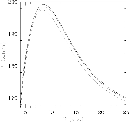
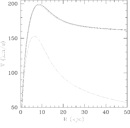
Figure 5: Bottom: exact Newtonian (dot-dashed line), classical MOND (dashed line), and T$e$V$e$S (full line) equatorial-plane rotation curves for a disk galaxy model with density distribution given in equation (43). The dotted line is the corresponding rotation curve approximated using Eq.(1). The top panel is a zoom-in of the upper left corner of the bottom panel.

Here, for the first time in the literature, we compare the different computed rotation curves for the same disk galaxy using the prescriptions of Eq. (1) (Milgrom’s law), Eq. (11) (classical MOND), and Eq. (18) (or equivalently Eq. 42, i.e. T$e$V$e$S). We consider an exponential disk model typical of a high surface brightness galaxy, characterized by a baryonic density distribution

$$\rho_{b}(R,z)=\frac{M_{b}}{4\pi{R_{0}}^{2}z_{0}}{\exp\left(-\frac{R}{R_{0}}\right)(\cosh\frac{z}{z_{0}})^{-2}},$$ (43)

with total mass $M_{b}=4.2\times 10^{10}M_{\odot}$, and characteristic scale lengths $R_{0}=3\,{\rm kpc}$ and $z_{0}=0.1\,{\rm kpc}$, where $R$ and $z$ are the cylindrical coordinates.

We can compute the exact force field, by solving Eq. (11) using the numerical MOND potential solver developed by CLN . This solver was originally tested in CLN for the standard $\mu$-function of Eq. (3), but we verified it works as well in solving Eq. (11) for other $\mu$-functions such as Eq. (2) and Eq. (5), or in solving the scalar field Poisson equation for a $\mu_{s}$-function such as Eq. (33).

For this model we compute exactly four different equatorial-plane rotation curves, which are plotted in Fig. 5: the Newtonian rotation curve (dot-dashed), the classical MOND rotation curve for the simple $\mu$-function of Eq. (2)(dashed), and the T$e$V$e$S rotation curve for the $\mu_{s}$-function of Eq. (33) (full line; we assumed for this plot $a_{0}=1.2\times 10^{-8}$ cm s^-2). The MOND/T$e$V$e$S rotation curves deviate significantly from the Newtonian one even at small radii, which is characteristic of the simple function (see Sect. II). Fig. 5 also plots as a dotted line the approximated rotation curve calculated from Eq. (1) with the simple $\mu$-function. From the bottom panel of Fig. 5 it is apparent how for an exponential disk model the exact T$e$V$e$S rotation curve, the exact classical MOND rotation curve, and the corresponding approximated rotation curve are practically indistinguishable from an observational point of view. Only a zoom-in at intermediate radii (Fig. 5, top) allows to appreciate the difference between the three modified-gravity curves: the T$e$V$e$S curve is systematically slightly higher (by less than 0.5%) than the classical MOND one, while the approximated curve using Milgrom’s law slightly overestimates the velocity (by only a few tenth of percent) for $R<~{}2R_{0}$, and slightly underestimates it (by less than 1%) for $R>~{}2R_{0}$. Note that if we consider $R=25$ kpc as the typical last observed radius in this high surface brightness galaxy, the difference between the circular velocity at that point and the asymptotic one ($\sim$ 5-10 km/s) is in any case higher than the difference between the velocities predicted at that point from Milgrom’s law and from T$e$V$e$S due to the non-sphericity of the system ($\sim$ 1-2 km/s).

IV Cosmology

IV.1 The Cauchy problem

We have seen that the asymptotic condition $\mu(x)\sim x$ when $x\ll 1$ implies that $\mu_{s}(s)$ must behave linearly with $s$ when $s$ is small (Eq. 27), and notably that we must have $\mu_{s}(0)=0$. This $s=0$ signals the transition between local physics and cosmology in T$e$V$e$S Bekenstein2004 .

Let us however emphasize that a k-essence theory such as T$e$V$e$S can exhibit superluminal propagations whenever $f^{\prime\prime}(y)>0$ JPB06 . Although it does not threaten causality JPB06 , one has to check that the Cauchy problem is still well-posed for the field equations. Within the choice of signature $(-,+,+,+)$ of local Lorentzian metrics, it has been shown JPB06 ; Susskind ; Rendall that it requires the otherwise free function $f$ to satisfy the following properties, $\forall y$:

$$f^{\prime}(y)>0$$ (44)

$$f^{\prime}(y)+2yf^{\prime\prime}(y)>0.$$ (45)

In terms of the scalar field strength $s\equiv(c^{2}/la_{0})\sqrt{y/k}$ (when $y\geq 0$, for a quasi-static galaxy), and of the auxiliary function $\mu_{s}(s)\equiv 4\pi f^{\prime}(y)/k$ , these conditions read, $\forall s\geq 0$:

$$\mu_{s}(s)>0$$ (46)

$$\mu_{s}(s)+s\mu^{\prime}_{s}(s)>0.$$ (47)

where the prime denotes the derivative with respect to $s$. Note that, throughout Sect. III, although we have shown that it was sometimes impossible to recover a given $\mu$-function from any single-valued unbounded $\mu_{s}$-function, we implicitly assumed that for a given $\mu_{s}$ it was $always$ possible to recover a spherically symmetric formulation “à la Milgrom” of local physics of T$e$V$e$S, i.e. an equation like Eq. (20). This means that when inserting a given $\mu_{s}$ in Eq. (23), the inversion of $x(s)$ was assumed to be $always$ possible (i.e. $x(s)$ is strictly increasing). Making use of $\Xi>0$, this is actually $guaranteed$ by the second inequality above, meaning that $s\mu_{s}(s)$ must be a strictly increasing function of $s$.

Now, concerning the transition between local physics and cosmology in T$e$V$e$S, the asymptotic behaviour of the $\mu$-function can therefore not be implemented by a consistent k-essence theory, since $\mu_{s}(0)=0$ would violate both inequalities at $s=0$. As explained in JPB06 ; JPBGEF , all present day k-essence-like theories of MOND such as T$e$V$e$S predict the existence of a singular surface around each galaxies on which the scalar degree of freedom does not propagate, and can therefore not provide a consistent picture of collapsed matter embedded into a cosmological background.

A simple solution consists in assuming a modified asymptotic behaviour of the $\mu$-function, namely of the form

$$\mu(x)\sim\varepsilon_{0}+x$$ (48)

if $x\ll 1$. In that case there is a return to a Newtonian behaviour at a very low acceleration scale $x\ll\varepsilon_{0}$, and rotation curves of galaxies are only approximatively flat until the galactocentric radius

$$R\sim\frac{1}{\varepsilon_{0}}\sqrt{\frac{G_{N}M}{a_{0}}}.$$ (49)

One must thus have $\varepsilon_{0}\ll 1$. A similar phenomenology also arises in a slightly different context in Sanderseps . Present data on galaxy rotation curves Gen3741 suggest that $1/\varepsilon_{0}$ must be at least of the order of $10$. Note that $\varepsilon_{0}$ is a quantity which slowly evolves with cosmic time (such as $\nu_{0}$ and $a_{0}$). In order to have such a behaviour for $\mu$, one must have in the deep-MOND regime $\mu_{s}\sim s/\nu_{0}+\varepsilon$ for small $s$, and we then have $\varepsilon_{0}=\nu_{0}\varepsilon$ (where $\varepsilon$ is a constant).

Note that, in the negative range of values of $y$ corresponding to the time-like sector of the expanding Universe, $\mu_{s}$ can still be defined as a function of $y$ as in Eq. (19). It can also be viewed as a function of $s$ if we extend the definition of s to

$$s\equiv{\rm sign}(y)\frac{c^{2}}{la_{0}}\sqrt{\frac{|y|}{k}}.$$ (50)

Then the Cauchy conditions read, $\forall s\leq 0$:

$$\mu_{s}(s)>0$$ (51)

$$\mu_{s}(s)-s\mu^{\prime}_{s}(s)>0.$$ (52)

IV.2 The mirror-image function

To be able to describe both galaxies and cosmology, the free function of T$e$V$e$S must thus be able to deal also with non-stationary systems such as the Universe itself. We describe hereafter how this can be achieved, following ZF06 .

Bekenstein’s original proposal Bekenstein2004 was to construct the scalar field action of Eq. (13) whith a lagrangian density given as a one-to-one function of $\mu_{s}$ viewed as an auxiliary non-dynamical scalar field, i.e. $f(y)={\cal F}(\mu_{s})$.

Such one-to-one construction had the drawback that the lagrangian density of the scalar field necessarily had unphysical “gaps”, i.e. that a sector was reserved for space-like systems (e.g. from dwarf galaxies to the solar system in the range $0<\mu_{s}<\mu_{0}$ for $y>0$) and a disconnected sector was reserved for time-like systems (e.g., the expanding Universe in the range $\mu_{s}>2\mu_{0}$ for $y<0$). While viable mathematically, such a disconnected Universe would not permit galaxies to collapse continuously out of the Hubble expansion.

In an effort to re-connect galaxies with the expanding Universe in T$e$V$e$S, it was proposed in ZF06 to construct the lagrangian density as a one-to-one continuous function of $y$, rather than a function of $\mu_{s}$, thus not considering $\mu_{s}$ as an auxiliary non-dynamical scalar field anymore. This allows for a smooth transition from the edge of galaxies where $y\sim 0$ to the Hubble expansion. It was also suggested in ZF06 to extrapolate the lagrangian density for galaxies into the cosmological regime by simple mirror-imaging, to minimize any fine-tuning in T$e$V$e$S, i.e.

$$\mu_{s}(s)=\mu_{s}(-s)$$ (53)

with $s$ defined as in Eq. (50), meaning that the time-like sector is a simple mirror-image of the space-like sector.

In other words, it means that, in order to produce a consistent cosmological picture, we suggest to extend the $\alpha$-family of Eq. (34) to the time-like sector by using the following k-essence function $f(y)$ in the action of the scalar field (Eq. 13):

$$f(y)=f(0)+\int_{0}^{y}\frac{k\mu_{s}}{4\pi}{\rm d}y$$ (54)

with

$$\mu_{s}=\varepsilon+\frac{\sqrt{|y|}}{A_{0}-\alpha\sqrt{|y|}},~{}0<\varepsilon<0.1,~{}0\leq\alpha\leq 1,$$ (55)

where $A_{0}=\sqrt{3}k/4\pi$.

It would thus be of great interest to compute the CMB anisotropies and matter power spectrum Skordis ; Dodelson using this action for the scalar field allowing for a smooth transition from the edge of galaxies to the Hubble expansion. Note also that the integration constant $f(0)$ can play the role of the cosmological constant Hao ($f(0)=0$ corresponding to no cosmological constant), but that even a no-cosmological constant model could drive late-time acceleration Zcosmo ; Diaz , which is not surprising since k-essence scalar fields were first introduced to address the dark energy problem. This T$e$V$e$S cosmological model is thus worth exploring since it could have the ability to resolve many problems at the same time. However, the $\alpha$-family of $\mu$-functions does not work very well on galaxy cluster scales if ${\bf g}_{N}$ is the gravity generated by baryons alone in Eq. (42). This problem of the MOND-phenomenology has been known for a while Aguirre , and it was then suggested San2003 that ordinary neutrinos of 2 eV could be included in the “known matter-total gravity” relation. Including ${\bf g}_{N}$ as the gravity of both baryons and neutrinos, it was found in ASZF that a reasonable fit to the lensing of the now famous bullet cluster Clowe is possible if neutrinos have a 2 eV mass (a mass also invoked in current MOND fits of the CMB anisotropies Skordis ; McGCMB ), while the unusually high encounter speed of the bullet cluster bulvel could be reproduced since the modified gravity potentials are deeper than the usual CDM ones. This cosmological framework was called the $\mu$HDM paradigm in ASZF by contrast with the usual $\Lambda$CDM one. These neutrinos would not change the gravity on galaxy scales due to their low densities ASZF , hence would not affect the goodness of the rotation curves fits presented in Sect. II. However, for elliptical galaxies at the very center of galaxy clusters where the neutrino density is the highest, the velocity dispersion profiles could be affected by these neutrinos, thus explaining the poor purely baryonic fits for NGC 1399 when using Eq. (2) Richtler (even though the external field effect in this galaxy, due to the gravity of the cluster itself, might render the fits difficult to achieve in practice even when including neutrinos).

V Conclusions

Throughout this paper we have studied from a theoretical point of view the observationally motivated baryon-gravity relation in galaxies Don ; McG ; McGa . This relation is completely encapsulated within the $\mu$-function (see Eq. 1) of Modified Newtonian Dynamics Milgrom83 , each distinct function defining a distinct baryon-gravity relation. This relation might be empirical or fundamental, but the present-day success of the relation with the sole constraints of the MOND paradigm, i.e. $\mu(x)=1$ at $x\gg 1$ and $\mu(x)=x$ at $x\ll 1$ with $x\sim g/cH_{0}$, points at first sight to a modification of gravity in the ultra-weak field limit. Even though the most important aspect of MOND remains this asymptotic behaviour, the study of the transition between the Newtonian regime and the deep-MOND regime, characterized by the shape of the $\mu$-function, may also be important in the quest for a possible fundamental theory underpinning the MOND prescription. We have thus investigated the observational constraints upon the $\mu$-function in that transition zone, as well as the theoretical constraints upon it in the framework of the relativistic formulation of MOND dubbed T$e$V$e$S Bekenstein2004 . Note that the latter are only valid if MOND really has its basis in a multifield theory like T$e$V$e$S, which is of course far from guaranteed.

We have shown that:

i) Observationally (from the quality of galaxy rotation curves and the current accuracy of population synthesis models), one cannot distinguish between the “simple” (Eq. 2) and the “standard” (Eq. 3) form of the $\mu$-function, but the transition from Newton to MOND cannot be much more gradual than that implied by the simple function (Sect. II).

ii) The simple form of $\mu$ does require generally lower mass-to-light ratios for the stellar components of spiral galaxies than does the standard form. This could, combined with accurate population synthesis models, eventually distinguish between them (Sect. II).

iii) A particular class of T$e$V$e$S free functions (the unbounded $\mu_{s}$ functions in Eq. 18 and Eq. 19) correspond to a trivial renormalization of the gravitational constant $G_{N}=\Xi G$ where $\Xi$ is a parameter of the theory, and are easily linked to the $\mu$-function of MOND. However, this $\mu$-function must have $n\leq 1$ in its asymptotic expansion $\mu(x)\sim 1-A/x^{n}$ (where $A$ is some positive constant), meaning that the standard form of $\mu$ (Eq. 3) cannot be recovered from a single-valued unbounded $\mu_{s}$ (Sect. III D).

iv) Renormalizing the gravitational constant as $G_{N}=\nu_{0}G$ with $\nu_{0}>\Xi$ for bounded $\mu_{s}$ functions $allows$ to recover $\mu$-functions with a steeper asymptotic expansion. The standard $\mu$ of Eq. (3) can be recovered if $\nu_{0}$ is such that Eq. (41) is invertible (Sect. III E).

v) Observationally (from galaxy rotation curves) one cannot distinguish between Milgrom’s law Milgrom83 , classical MOND BM84 and T$e$V$e$S Bekenstein2004 . Using the code of CLN we have shown that the difference between the circular velocity at the last observed radius in a typical spiral galaxy and the asymptotic circular velocity is higher than the difference between the velocities predicted at that point from classical MOND and from T$e$V$e$S due to the non-sphericity of the system (Sect. III F).

vi) Some modification of the $\mu$-function is necessary to make cosmology consistent with quasi-static mass distributions in T$e$V$e$S, which should lead to a return to $1/r^{2}$ attraction at very low accelerations in galaxies (Sect. IV A).

vii) By extrapolating the scalar field lagrangian density for galaxies into the cosmological regime by simple mirror-imaging in T$e$V$e$S, one minimizes the fine-tuning of the theory while avoiding that the sector reserved for space-like systems such as galaxies be disconnected from the sector reserved for time-like systems such as the Universe itself (Sect. IV B).

Let us finally note that the simple form of $\mu$ (Eq. 2), yielding excellent fits to galaxy rotation curves and not needing a non-trivial renormalization of the gravitational constant in T$e$V$e$S, has to be distorded in the limit of high accelerations to be in accordance with observed planetary motions in the inner solar system sanderssolar . This could be achieved for an unbounded $\mu_{s}$ by e.g. somehow making the parameter $\alpha$ dynamical in Eq. (34), going smoothly from 1 in galaxies towards 20 at the orbit of Mercury. More prosaically, it can be achieved by making the $\mu_{s}$ function bounded as in the $n=1$ case of (ZF06, , eq.(13)).

- (1) D.N. Spergel, R. Bean, O. Dore, et al., astro-ph/0603449 (2006)
- (2) D. Clowe, M. Bradac, A.H. Gonzalez, et al., Astrophys.J. 648, L109 (2006)
- (3) N. Bissantz, P. Englmaier, O. Gerhard, Mon. Not. Roy. Astron. Soc. 340, 949 (2003)
- (4) B. Famaey, J. Binney, Mon. Not. Roy. Astron. Soc. 363, 603 (2005)
- (5) J. Diemand, M. Zemp, B. Moore, et al., Mon. Not. Roy. Astron. Soc. 364, 665 (2005)
- (6) Y.P. Jing, Y. Suto, Astrophys. J. 574, 538 (2002)
- (7) R.A. Swaters, B.F. Madore, F.C. van den Bosch, et al., Astrophys. J. 583, 732 (2003)
- (8) W.J.G. de Blok, A. Bosma, Astron. Astrophys. 385, 816 (2002)
- (9) G. Gentile, P. Salucci, U. Klein, et al., Mon. Not. Roy. Astron. Soc. 351, 903 (2004)
- (10) G. Gentile, A. Burkert, P. Salucci, et al., Astrophys. J. 634, L145 (2005)
- (11) J.D. Simon, A.D. Bolatto, A. Leroy, et al., Astrophys. J. 621, 757 (2005)
- (12) R. Kuzio de Naray, S. McGaugh, W.J.G. de Blok, A. Bosma, Astrophys. J. Supp. 165, 461 (2006)
- (13) B. Moore, S. Ghigna, F. Governato, et al., Astrophys. J. 524, L19 (1999)
- (14) F. Donato, G. Gentile, P. Salucci, Mon. Not. Roy. Astron. Soc. 353, L17 (2004)
- (15) S. McGaugh, Phys. Rev. Lett. 95 171302 (2005)
- (16) S. McGaugh, W.J.G. de Blok, J.M. Schombert, et al., astro-ph/0612410 (2006)
- (17) A.H. Broeils, Astron. Astrophys. 256, 19 (1992)
- (18) M. Milgrom, Astrophys. J. 270, 365 (1983)
- (19) M. Milgrom, Astrophys. J. 270, 371 (1983)
- (20) M. Milgrom, Astrophys. J. 270, 384 (1983)
- (21) M. Milgrom, EAS Publications Series 20, 217 (2006)
- (22) L. Blanchet, astro-ph/0605637 (2006)
- (23) L. Blanchet, gr-qc/0609121 (2006)
- (24) J. Bekenstein, M. Milgrom, Astrophys. J. 286, 7 (1984)
- (25) J. Bekenstein, Phys. Rev. D 70, 083509 (2004)
- (26) L. Ciotti, J. Binney, Mon. Not. Roy. Astron. Soc. 351, 285 (2004)
- (27) F.J. Sánchez-Salcedo, J. Reyes-Iturbide, X. Hernandez, Mon. Not. Roy. Astron. Soc. 370, 1829 (2006)
- (28) H.S. Zhao, Astron. Astrophys. 444, L25 (2005)
- (29) H.S. Zhao, L.L. Tian, Astron. Astrophys. 450, 1005 (2006)
- (30) M. Milgrom, Annals Phys. 229, 384 (1994)
- (31) M. Milgrom, Phys. Lett. A 253, 273 (1999)
- (32) R.B. Tully, J.R. Fisher, Astron. Astrophys. 54, 661 (1977)
- (33) S. McGaugh, Astrophys. J. 632, 859 (2005)
- (34) R.H. Sanders, S. McGaugh, Ann. Rev. Astron. Astrophys. 40, 263 (2002)
- (35) G.W. Angus, B. Famaey, H.S. Zhao, Mon. Not. Roy. Astron. Soc. 371, 138 (2006)
- (36) R.H. Sanders, Mon. Not. Roy. Astron. Soc. 370, 1519 (2006)
- (37) K.G. Begeman, A.H. Broeils, R.H. Sanders, Mon. Not. Roy. Astron. Soc. 249, 523 (1991)
- (38) R. Bottema, J.L.G. Pestana, B. Rothberg, R.H. Sanders, Astron. Astrophys. 393, 453 (2002)
- (39) Y. Schuberth, T. Richtler, B. Dirsch, et al., Astron. Astrophys. 459, 391 (2006)
- (40) R.S. de Jong, E. Bell, astro-ph/0604391 (2006)
- (41) E. Bell, R.S. de Jong, Astrophys. J. 550, 212 (2001)
- (42) E. Bell, D.F. McIntosh, N. Katz, M.D. Weinberg, Astrophys. J. Supp. 149, 289 (2003)
- (43) R. Brada, M. Milgrom, Astrophys. J. 519, 590 (1999)
- (44) L. Ciotti, P. Londrillo, C. Nipoti, Astrophys. J. 640, 741 (2006)
- (45) O. Tiret, F. Combes, astro-ph/0701011 (2007)
- (46) R. Brada, M. Milgrom, Mon. Not. Roy. Astron. Soc. 276, 453 (1995)
- (47) T.G. Zlosnik, P.G. Ferreira, G.D. Starkman, Phys. Rev. D 74, 044037 (2006)
- (48) C. Armendáriz-Picón, T. Damour, V. Mukhanov, Phys. Lett. B 458, 219 (1999)
- (49) T. Chiba, T. Okabe, M. Yamaguchi, Phys. Rev D 62, 023511 (2000)
- (50) C. Armendáriz-Picón, V. Mukhanov, P.J. Steinhardt, Phys. Rev D 63, 103510 (2001)
- (51) M. Cadoni, Gen. Rel. Grav. 36, 2681 (2004)
- (52) Y. Sobouti, astro-ph/0603302 (2006)
- (53) S. Capozziello, V.F. Cardone, A. Troisi, astro-ph/0603522 (2006)
- (54) M. Persic, P. Salucci, F. Stel, Mon. Not. Roy. Astron. Soc. 281, 27 (1996)
- (55) P. Salucci, G. Gentile, Phys. Rev. D 73, 128501 (2006)
- (56) H.S. Zhao, B. Famaey, Astrophys. J. 638, L9 (2006)
- (57) J.-P. Bruneton, G. Esposito-Farèse, Field-theoretical formulations of MOND-like gravity, in preparation
- (58) J.-P. Bruneton, gr-qc/0607055 (2006)
- (59) Y. Aharonov, A. Komar, L. Susskind, Phys. Rev. 182, 1400 (1969)
- (60) A.D. Rendall, Class. Quant. Grav. 23, 1557 (2006)
- (61) R.H. Sanders, Mon. Not. Roy. Astron. Soc. 223, 539 (1986)
- (62) G. Gentile, P. Salucci, U. Klein, G.L. Granato, Mon. Not. Roy. Astron. Soc. in press, astro-ph/0611355 (2007)
- (63) C. Skordis, D.F. Mota, P.G. Ferreira, C. Boehm, Phys. Rev. Lett. 96, 011301 (2006)
- (64) S. Dodelson, M. Liguori, astro-ph/0608602 (2006)
- (65) J.G. Hao, R. Akhoury, astro-ph/0504130 (2005)
- (66) H.S. Zhao, astro-ph/0610056 (2006)
- (67) L.M. Diaz-Rivera, L. Samushia, B. Ratra, Phys. Rev. D 73, 083503 (2006)
- (68) A. Aguirre, J. Schaye, E. Quataert, Astrophys. J. 561, 550 (2001)
- (69) R.H. Sanders, Mon. Not. Roy. Astron. Soc. 342, 901 (2003)
- (70) G.W. Angus, H.Y. Shan, H.S. Zhao, B. Famaey, Astrophys.J. 654, L13 (2007)
- (71) S. McGaugh, Astrophys. J. 611, 26 (2004)
- (72) G.R. Farrar, R.A. Rosen, astro-ph/0610298 (2006)
- (73) T. Richtler, Y. Schuberth, A. Romanowsky, Rev. Mex. Astron. Astrofís. 26, 198 (2006)