Radial profile and log-normal fluctuations of intra-cluster medium as an origin of systematic bias of spectroscopic temperature

Abstract

The origin of the recently reported systematic bias in the spectroscopic temperature of galaxy clusters is investigated using cosmological hydrodynamical simulations. We find that the local inhomogeneities of the gas temperature and density, after corrected for the global radial profiles, have nearly a universal distribution that resembles the log-normal function. Based on this log-normal approximation for the fluctuations in the intra-cluster medium, we develop an analytical model that explains the bias in the spectroscopic temperature discovered recently. We conclude that the multi-phase nature of the intra-cluster medium not only from the radial profiles but also from the local inhomogeneities plays an essential role in producing the systematic bias.

1. Introduction

Recent progress both in numerical simulations and observations has improved physical modeling of galaxy clusters beyond a simple isothermal and spherical approximation for a variety of astrophysical and cosmological applications; departure from isothermal distribution was discussed in the context of the Sunyaev-Zel’dovich effect (Inagaki, Suginohara & Suto, 1995; Yoshikawa, Itoh & Suto, 1998; Yoshikawa & Suto, 1999), an empirical $\beta$-model profile has been replaced by that based on the NFW dark matter density profile (Navarro, Frenk, & White, 1997; Makino, Sasaki & Suto, 1998; Suto, Sasaki, & Makino, 1998), non-spherical effects of dark halos have been considered fairly extensively (Lee & Shandarin, 1998; Sheth & Tormen, 1999; Jing & Suto, 2002; Lee & Suto, 2003, 2004; Kasun & Evrard, 2005), and the physical model for the origin of the triaxial density profile has been proposed (Lee, Jing & Suto, 2005).

Despite an extensive list of the previous studies, no physical model has been proposed for the statistical nature of underlying inhomogeneities in the intra-cluster medium (ICM, hereafter). Given the high spatial resolutions achieved both in observations and simulations, such a modeling should play a vital role in improving our understanding of galaxy clusters, which we will attempt to do in this paper.

Temperature of the ICM is one of the most important quantities that characterize the cluster. In X-ray observations, the spectroscopic temperature, $T_{\mathrm{spec}}$, is estimated by fitting the thermal continuum and the emission lines of the spectrum. In the presence of inhomogeneities in the ICM, the temperature so measured is inevitably an averaged quantity over a finite sky area and the line-of-sight. It has been conventionally assumed that $T_{\mathrm{spec}}$ is approximately equal to the emission-weighted temperature:

$$T_{\mathrm{ew}}\equiv\frac{\int n^{2}\Lambda(T)TdV}{\int n^{2}\Lambda(T)dV},$$ (1)

where $n$ is the gas number density, $T$ is the gas temperature, and $\Lambda$ is the cooling function. Mazzotta et al. (2004), however, have pointed out that $T_{\mathrm{spec}}$ is systematically lower than $T_{\mathrm{ew}}$. The authors have proposed an alternative definition for the average, spectroscopic-like temperature, as

$$T_{\mathrm{sl}}\equiv\frac{\int n^{2}T^{a-1/2}dV}{\int n^{2}T^{a-3/2}dV}.$$ (2)

They find that $T_{\mathrm{sl}}$ with $a=0.75$ reproduces $T_{\mathrm{spec}}$ within a few percent for simulated clusters hotter than a few keV, assuming Chandra or XMM-Newton detector response functions. Rasia et al. (2005) performed a more systematic study of the relation between $T_{\mathrm{ew}}$ and $T_{\mathrm{sl}}$ using a sample of clusters from SPH simulations and concluded that $T_{\mathrm{sl}}\sim 0.7T_{\mathrm{ew}}$. Vikhlinin (2006) provided a useful numerical routine to compute $T_{\mathrm{sl}}$ down to ICM temperatures of $\sim 0.5$ keV with an arbitrary metallicity. It should be noted that $T_{\mathrm{ew}}$ is not directly observable, although it is easily obtained from simulations.

The above bias in the cluster temperature should be properly taken into account when confronting observational data with theory, for example, in cosmological studies. As noted by Rasia et al. (2005), it can result in the offset in the mass-temperature relation of galaxy clusters. Shimizu et al. (2006) have studied its impact on the estimation of the mass fluctuation amplitude at $8h^{-1}$Mpc, $\sigma_{8}$. The authors perform the statistical analysis using the latest X-ray cluster sample and find that $\sigma_{8}\sim 0.76\pm 0.01+0.50(1-\alpha_{M})$, where $\alpha_{M}=T_{\mathrm{spec}}/T_{\mathrm{ew}}$. The systematic difference of $T_{\mathrm{spec}}\sim 0.7T_{\mathrm{ew}}$ can thus shift $\sigma_{8}$ by $\sim 0.15$.

In this paper, we aim to explore the origin of the bias in the spectroscopic temperature by studying in detail the nature of inhomogeneities in the ICM. We investigate both the large-scale gradient and the small-scale variations of the gas density and temperature based on the cosmological hydrodynamical simulations. Having found that the small-scale density and temperature fluctuations approximately follow the log-normal distributions, we construct an analytical model for the local ICM inhomogeneities that can simultaneously explain the systematic bias.

The plan of this paper is as follows. In §2, we describe our simulation data, construct the mock spectra and compare quantitatively the spectroscopic temperature with the emission-weighted temperature and the spectroscopic-like temperature suggested by Mazzotta et al. (2004). In §3, we propose an analytical model for the inhomogeneities in the ICM. In §4, we test our model against the result of the simulation. Finally, we summarize our conclusions in §5. Throughout the paper, temperatures are measured in units of keV.

2. The Bias in the Spectroscopic Temperature

2.1. Cosmological Hydrodynamical Simulation

The results presented in this paper have been obtained by using the final output of the Smoothing Particle Hydrodynamic (SPH) simulation of the local universe performed by Dolag et al. (2005). The initial conditions were similar to those adopted by Mathis et al. (2002) in their study (based on a pure N-body simulation) of structure formation in the local universe. The simulation assumes the spatially–flat $\Lambda$ cold dark matter ($\Lambda$ CDM) universe with a present matter density parameter $\Omega_{0m}=0.3$, a dimensionless Hubble parameter $h=H_{0}/100~{}{\rm km~{}s^{-1}~{}Mpc^{-1}}=0.7$, an rms density fluctuation amplitude $\sigma_{8}=0.9$ and a baryon density parameter $\Omega_{\rm b}=0.04$. Both the number of dark matter and SPH particles are $\sim 50$ million within the high-resolution sphere of radius $\sim 110$ Mpc which is embedded in a periodic box of $\sim 343$ Mpc on a side, filled with nearly 7 million low-resolution dark matter particles. The simulation is designed to reproduce the matter distribution of the local Universe by adopting the initial conditions based on the IRAS galaxy distribution smoothed on a scale of 7 Mpc (see Mathis et al., 2002, for detail).

The run has been carried out with GADGET-2 (Springel, 2005), a new version of the parallel Tree-SPH simulation code GADGET (Springel et al., 2001). The code uses an entropy-conserving formulation of SPH (Springel & Hernquist, 2002), and allows a treatment of radiative cooling, heating by a UV background, and star formation and feedback processes. The latter is based on a sub-resolution model for the multiphase structure of the interstellar medium (Springel & Hernquist, 2003); in short, each SPH particle is assumed to represent a two-phase fluid consisting of cold clouds and ambient hot gas.

The code also follows the pattern of metal production from the past history of cosmic star formation (Tornatore et al., 2004). This is done by computing the contributions from both Type-II and Type-Ia supernovae and energy feedback and metals are released gradually in time, accordingly to the appropriate lifetimes of the different stellar populations. This treatment also includes in a self-consistent way the dependence of the gas cooling on the local metallicity. The feedback scheme assumes a Salpeter IMF (Salpeter, 1955) and its parameters have been fixed to get a wind velocity of $\approx 480$ $\mathrm{km~{}s^{-1}}$. In a typical massive cluster the SNe (II and Ia) add to the ICM as feedback $\approx 2$ keV per particle in an Hubble time (assuming a cosmological mixture of H and He); $\approx 25$ per cent of this energy goes into winds. A more detailed discussion of cluster properties and metal distribution within the ICM as resulting in simulations including the metal enrichment feedback scheme can be found in Tornatore et al. (2004). The simulation provides the metallicities of the six different species for each SPH particle. Given the fact that the major question that we addressed is not the accurate estimate of $T_{\mathrm{spec}}$ or $T_{\mathrm{sl}}$, but the systematic difference between the two, we decided to avoid the unnecessary complication and simply to assume the constant metallicity. Therefore we adopt a constant metallicity of 0.3 $Z_{\odot}$ in constructing mock spectra below, and the MEKAL (not VMEKAL) model for the spectral fitting.

The gravitational force resolution (i.e. the comoving softening length) of the simulations has been fixed to be 14 kpc (Plummer-equivalent), which is comparable to the inter-particle separation reached by the SPH particles in the dense centers of our simulated galaxy clusters.

2.2. Mock Spectra of Simulated Clusters

Among the most massive clusters formed within the simulation we extracted six mock galaxy clusters, contrived to resemble A3627, Hydra, Perseus, Virgo, Coma, and Centaurus, respectively. Table 1 lists the observed and simulated values of the total mass and the radius of these clusters. In order to specify the degree of the bias in our simulated clusters, we create the mock spectra and compute $T_{\mathrm{spec}}$ in the following manner.

First, we extract a $3h^{-1}~{}\mathrm{Mpc}$ cubic region around the center of a simulated cluster and divide it into $256^{3}$ cells so that the size of each cell is approximately equal to the gravitational softening length mentioned above. The center of each cluster is assigned so that the center of a sphere with radius $1h^{-1}~{}\mathrm{Mpc}$ equals to the center of mass of dark matter and baryon within the sphere.

The gas density and temperature of each mesh point (labeled by $I$) are calculated using the SPH particles as

$$\rho_{I}=\sum_{i=1}^{Ngas}m_{i}W(|{\boldsymbol{r}}_{I}-{\boldsymbol{r}}_{i}|,h_{i}),$$ (3)

$$T_{I}=\sum_{i=1}^{Ngas}\frac{m_{i}T_{i}}{\rho_{i}}W(|{\boldsymbol{r}}_{I}-{\boldsymbol{r}}_{i}|,h_{i}),$$ (4)

where ${\boldsymbol{r}}_{I}$ is the position of the mesh point, $W$ denotes the smoothing kernel, and $m_{i}$, ${\boldsymbol{r}}_{i}$, $h_{i}$, $T_{i}$, and $\rho_{i}$ are the mass associated with the hot phase, position, smoothing length, temperature, and density associated with the hot gas phase of the $i$-th SPH particle, respectively. We adopt the smoothing kernel:

$$W(|{\boldsymbol{r}}_{I}-{\boldsymbol{r}}_{i}|,h_{i})=\frac{1}{\pi h_{i}^{3}}\left\{\begin{array}[]{lr}1-(3/2)u^{2}+(3/4)u^{3}&\mbox{if $0\leq u\leq 1$}\\ (2-u)^{3}/4&\mbox{if $1\leq u\leq 2$}\\ 0&\mbox{otherwise,}\\ \end{array}\right.$$ (8)

where $u\equiv|{\boldsymbol{r}}_{I}-{\boldsymbol{r}}_{i}|/h_{i}$.

It should be noted that the current implementation of the SPH simulation results in a small fraction of SPH particles that have unphysical temperatures and densities. This is shown in the temperature – density scatter plot of Figure 1. The red points correspond to SPH particles that should be sufficiently cooled, but not here because of the limited resolution of the simulation. Thus if they satisfy the Jean criterion, they should be regarded as simply cold clumps without retaining the hot gas nature; see Figure 1 and section 2.1 of Yoshikawa et al. (2001). In contrast, the blue points represent the SPH particles that have experienced the cooling catastrophe, and have significantly high cold gas fraction (larger than 10 percent). In either case, they are not supposed to contribute the X-ray emission. Thus we remove their spurious contribution to the X-ray emission and the temperature estimate of ICM. Specifically we follow Borgani et al. (2004), and exclude particles (red points) with $T_{i}<3\times 10^{4}\mathrm{K}$ and $\rho_{i}>500\rho_{\rm c}\Omega_{\rm b}$ , where $\rho_{\rm c}$ is the critical density, and particles (blue points) with more than ten percent mass fraction of the cold phase. While the total mass of the excluded particles is very small ($\sim 1\%$), they occupy a specific region in the $\rho$-$T$ plane and leave some spurious signal due to high density, in particular for blue points.

Second, we compute the photon flux $f(E)$ from the mesh points within the radius $r_{200}$ from the cluster center as

$$f(E)\,dE\propto\exp{(-\sigma_{gal}(E)N_{H})}\sum_{I\in r_{200}}\frac{\rho_{I}^{2}}{4\pi(1+z_{\mathrm{cl}})^{4}}\left(\frac{X}{m_{\mathrm{p}}^{2}}\right)\,P_{\mathrm{em}}(T_{I},Z,E(1+z_{\mathrm{cl}}))\,dE(1+z_{\mathrm{cl}}),$$ (9)

where $z_{\mathrm{cl}}$ denotes the redshift of the simulated cluster, $Z$ is the metallicity (we adopt 0.3 $Z_{\odot}$), $X$ is the hydrogen mass fraction, $m_{p}$ is the proton mass and $P_{\mathrm{em}}(T_{I},Z,E)$ is the emissivity assuming collisional ionization equilibrium. We calculate $P_{\mathrm{em}}(T_{I},Z,E)$ using SPEX 2.0. The term $\exp{(-\sigma_{gal}N_{H})}$ represents the galactic extinction; $N_{H}$ is the column density of hydrogen and $\sigma_{gal}(E)$ is the absorption cross section of Morrison & McCammon (1983). Since we are interested in the effect due to the spectrum distortion, not statistical error, we adopt a long exposure time as the total photon counts ${\cal N}=\int_{E=0.5~{}\mathrm{keV}}^{E=10~{}\mathrm{keV}}Ef(E)\,dE\sim$ 500,000. In this paper, we consider mock observations using Chandra and XMM-Newton, thus we neglect a peculiar velocity of the cluster and a turbulent velocity in ICM because of insufficient energy resolution of Chandra ACIS-S3 and XMM-Newton MOS1 detector.

Finally, the mock observed spectra are created by XSPEC version 12.0. We consider three cases for the detector response corresponding to 1) perfect response, 2) Chandra ACIS-S3, and 3) XMM-Newton MOS1. In the first case, we also assume no galactic extinction ($N_{H}=0$) and refer to it as an “IDEAL” case. In the second and third cases, we adopt an observed value to $N_{H}$ listed in Table 1 and redistribute the photon counts of the detector channel according to RMF (redistribution matrix file) of ACIS-S3 and MOS1 using the rejection method.

Figure 2 illustrates the mock spectra of “Virgo” and “Perseus” using RMF of ACIS-S3. Unless stated otherwise, we fit the spectra by an absorbed single-temperature MEKAL model in the energy band 0.5-10.0 keV. We define the spectroscopic temperature, $T_{\mathrm{spec}}$, as the best-fit temperature provided by this procedure. Since the spatial resolution of the current simulations is not sufficient to fully resolve the cooling central regions, a single-temperature model yields a reasonable fit to the mock spectra. For comparison, we also plot the spectra for a single temperature corresponding to the “emission weighted” value of the mesh points within $r_{200}$:

$$T_{\mathrm{ew}}^{\mathrm{sim,m}}=\frac{\sum_{I\in r_{200}}\rho_{I}^{2}T_{I}\Lambda(T_{I})}{\sum_{I\in r_{200}}\rho_{I}^{2}\Lambda(T_{I})}.$$ (10)

We calculate the cooling function $\Lambda(T)$ using SPEX 2.0 assuming collisional ionization equilibrium, the energy range of 0.5-10.0 keV, and the metallicity $0.3Z_{\odot}$. The difference between $T_{\mathrm{spec}}$ and $T_{\mathrm{ew}}^{\mathrm{sim,m}}$ is clearly distinguishable on the spectral basis in the current detectors.

Figure 3 shows the relation between $T_{\mathrm{spec}}$ and $T_{\mathrm{ew}}$ for our sample of simulated clusters. It is well represented by a linear relation $T_{\mathrm{spec}}=kT_{\mathrm{ew}}+l$ with the fitted values of $k=0.84,l=0.34$ (IDEAL), $k=0.84,l=0.36$ (ACIS) and $k=0.85,l=0.31$ (MOS), respectively. In the range of temperatures corresponding to rich clusters, the spectroscopic temperature $T_{\mathrm{spec}}$ is systematically lower than $T_{\mathrm{ew}}$ by $10-20$ %.

We note that the above bias should depend on the energy band in which $T_{\mathrm{spec}}$ is evaluated. In order to demonstrate it quantitatively, we also list in Table 1 the fitted values of $T_{\mathrm{spec}}$ from the 0.1-2.4 keV and 2.0-10.0 keV data, respectively. Because the exponential tail of the thermal bremsstrahlung spectrum from hotter components has negligible contribution in the softer band, the bias tends to increase and decrease in the softer and harder bands, respectively.

2.3. Spectroscopic-Like Temperature

In order to better approximate $T_{\mathrm{spec}}$, Mazzotta et al. (2004) proposed a “ spectroscopic-like temperature”; they found that equation (2) with $a=0.75$ reproduces $T_{\mathrm{spec}}$ in the 0.5-10.0 keV band within a few percent. Throughout this paper, we adopt $a=0.75$ when we estimate the spectroscopic-like temperature quantitatively. In Figure 3, we also plot this quantity computed from the mesh points within $r_{200}$:

$$T_{\mathrm{sl}}^{\mathrm{sim,m}}=\frac{\sum_{I\in r_{200}}\rho_{I}^{2}T_{I}^{0.25}}{\sum_{I\in r_{200}}\rho_{I}^{2}T^{-0.75}_{I}}.$$ (11)

As indicated in the bottom panel, $T_{\mathrm{sl}}^{\mathrm{sim,m}}$ reproduces $T_{\mathrm{spec}}$ within 6 % for all the simulated clusters in our sample. Given this agreement, we hereafter use $T_{\mathrm{sl}}^{\mathrm{sim,m}}$ to represent $T_{\mathrm{spec}}$, and express the bias in the spectroscopic temperature by

$$\kappa_{\mathrm{sim}}\equiv T_{\mathrm{sl}}^{\mathrm{sim,m}}/T_{\mathrm{ew}}^{\mathrm{sim,m}}.$$ (12)

Table 1 provides $\kappa_{\mathrm{sim}}$ (mesh-wise) for the six simulated clusters. The range of $\kappa_{\mathrm{sim}}$ (mesh-wise) is approximately 0.8-0.9. While $\kappa_{\mathrm{sim}}$ is systematically lower than unity, the value is somewhat higher than the results of Rasia et al. (2005), $T_{\mathrm{sl}}\sim 0.7T_{\mathrm{ew}}$. This is likely due to the different physics incorporated in the simulations and the difference in how $T_{\mathrm{sl}}$ and $T_{\mathrm{ew}}$ are computed from the simulation outputs. The major difference of the physics is the amplitude of the wind velocity employed; Rasia et al. (2005) used have a feedback with weaker wind of $340\mathrm{km\,s^{-1}}$, while our current simulations adopt a higher value of $480\mathrm{km\,s^{-1}}$. Because weaker wind cannot remove small cold blobs effectively, the value of $T_{\mathrm{sl}}/T_{\mathrm{ew}}$ of Rasia et al. (2005) is expected to be larger.

To show the difference of the temperature computation scheme explicitly, we also list in Table 1 the values of $\kappa_{\mathrm{sim}}\equiv T_{\mathrm{sl}}^{\mathrm{sim,p}}/T_{\mathrm{ew}}^{\mathrm{sim,p}}$ (particle-wise) computed in the “particle-wise” definitions used in Rasia et al. (2005):

$$T_{\mathrm{ew}}^{\mathrm{sim,p}}=\frac{\sum_{i\in r_{200}}m_{i}\rho_{i}\Lambda(T_{i})T_{i}}{\sum_{i\in r_{200}}m_{i}\rho_{i}\Lambda(T_{i})},$$ (13)

and

$$T_{\mathrm{sl}}^{\mathrm{sim,p}}=\frac{\sum_{i\in r_{200}}m_{i}\rho_{i}T_{i}^{0.25}}{\sum_{i\in r_{200}}m_{i}\rho_{i}T_{i}^{-0.75}},$$ (14)

(see also Borgani et al., 2004). In practice, the emission-weighted and spectroscopic-like temperatures defined in equation (13) and equation (14) are sensitive to a small number of cold (and dense) SPH particles present, while their contribution is negligible in the mesh-wise definitions, equation (10) and equation (11). As in Rasia et al. (2005), we have removed the SPH particles below a threshold temperature $T_{lim}=0.5$ keV to compute $\kappa_{\mathrm{sim}}$ (particle-wise). Table 1 indicates that $\kappa_{\mathrm{sim}}$ (particle-wise) tends to be systematically smaller than $\kappa_{\mathrm{sim}}$ (mesh-wise). Even adopting $T_{lim}=0.01$ keV makes $\kappa_{\mathrm{sim}}$ (particle-wise) smaller only by a few percent.

Given the limit of the particle-wise definitions mentioned above, we use the mesh-wise definitions of the emission-weighted temperature ($T_{\mathrm{ew}}^{\mathrm{sim,m}}$) and the spectroscopic-like temperature ($T_{\mathrm{sl}}^{\mathrm{sim,m}}$) given in equation (10) and (11), respectively, in the following sections.

3. Origin of the Bias in the Spectroscopic Temperature

3.1. Radial Profile and Log-normal Distribution of Temperature and Density

Having quantified the bias in the temperature of simulated clusters, we investigate its physical origin in greater detail. Since clusters in general exhibit inhomogeneities over various scales, we begin with segregating the large-scale gradient and the small-scale fluctuations of the gas density and temperature.

For the large-scale gradient, we use the radially averaged profile of the gas temperature and density shown in Figure 4. We divide the simulated clusters into spherical shells with a width of $67h^{-1}~{}\mathrm{kpc}$ and calculate the average temperature $T(r)$ and density $n(r)$ in each shell. The density profile $n(r)$ is fitted to the conventional beta model given by

$$n(r)=n_{0}\,\left[\frac{1}{1+(r/r_{c})^{2}}\right]^{3\beta/2},$$ (15)

where $n_{0}$ is the central density, $r_{c}$ is the core radius, and $\beta$ is the beta index. We adopt for the temperature profile $T(r)$ the polytropic form of

$$T(r)=T_{0}\,[n(r)/n_{0}]^{\gamma-1},$$ (16)

where $T_{0}$ is the temperature at $r=0$, and $\gamma$ is the polytrope index. The simulated profiles show reasonable agreement with the above models. The best-fit values of $\beta$ and $\gamma$ are listed in Table 1. The range of $\gamma$ is approximately 1.1-1.2.

In addition to their radial gradients, the gas density and temperature have small-scale fluctuations. Figure 5 illustrates the distributions of the gas density and temperature in each radial shell normalized by their averaged quantities,$\langle T\rangle$ and $\langle n\rangle$, respectively. Despite some variations among different shells, we find a striking similarity in the overall shape of the distributions. They approximately follow the log-normal distribution given by

$$P_{\mathrm{LN}}(\delta_{x})\,d\,\delta_{x}=\frac{1}{\sqrt{2\pi}\sigma_{\mathrm{LN},\,x}}\exp{\left[\frac{-\left(\log{\delta_{x}}+\sigma_{\mathrm{LN},\,x}^{2}/2\right)^{2}}{2\sigma_{\mathrm{LN},\,x}^{2}}\right]}\,\frac{d\delta_{x}}{\delta_{x}},$$ (17)

where $\delta_{x}\equiv x/\langle x\rangle$ and $x$ denotes $T$ or $n$ ($\delta_{T}\equiv T/\langle T\rangle$,$\delta_{n}\equiv n/\langle n\rangle$). For simplicity, we neglect the variations among different shells and fit the distribution for the whole cluster within $r_{200}$ (solid line) by the above equation (dashed line). The best-fit values of $\sigma_{\mathrm{LN},\,T}$ and $\sigma_{\mathrm{LN},\,n}$ are listed in Table 1.

The small-scale fluctuations mentioned above are not likely an artifact of the SPH scheme. We have applied the similar analysis to the data of grid-based simulations (D.Ryu, private communication) and obtained essentially the same results. Thus the log-normal nature of the fluctuations is physical, rather than numerical.

3.2. Analytical Model

Based on the distributions of gas density and temperature described in §3.1, we develop an analytical model to describe the contributions of the radial profile (RP) and the local inhomogeneities (LI) to the bias in the spectroscopic temperature.

To describe the emission-weighted and spectroscopic-like temperatures in simple forms, let us define a quantity:

$$A_{\alpha} \equiv \int n({\boldsymbol{r}})^{2}T({\boldsymbol{r}})^{\alpha}\,d{\bf r},$$ (18)

$$= \int_{0}^{R}r^{2}dr\,\int d\Omega\,n^{2}({\bf r})T^{\alpha}({\bf r}),$$

where the second line is for the spherical coordinate and $R$ denotes the maximum radius considered here (we adopt $R=r_{\mathrm{200}}$). Using this quantity, we can write down $T_{\mathrm{sl}}$ via equation (2) as

$$T_{\mathrm{sl}}^{\mathrm{model}}=A_{a-1/2}/A_{a-3/2}.$$ (19)

When the temperature is higher than $\sim 3$ keV, the cooling function is dominated by the thermal bremsstrahlung; $\Lambda\propto\sqrt{T}$. We find that substitution $\sqrt{T}$ for $\Lambda(T)$ yields only $\sim 1\%$ difference for the simulated clusters. In the present model, we adopt for simplicity the thermal bremsstrahlung cooling function, $\Lambda\propto\sqrt{T}$, and then equation (1) reduces to

$$T_{\mathrm{ew}}^{\mathrm{model}}=A_{3/2}/A_{1/2}.$$ (20)

When evaluating equation (18), we replace the spatial average with the ensemble average:

$$\int d\Omega\,n^{2}({\bf r})T^{\alpha}({\bf r}) = 4\pi[\langle n\rangle(r)]^{2}[\langle T\rangle(r)]^{\alpha}\int\int\delta_{n}^{2}\delta_{T}^{\alpha}P(\delta_{n},\delta_{T};r)d\delta_{n}d\delta_{T},$$ (21)

where $P(\delta_{n},\delta_{T};r)$ is a joint probability density function at $r$. Assuming further that the temperature inhomogeneity is uncorrelated with that of density, i.e. $P(\delta_{n},\delta_{T};r)=P(\delta_{n};r)\,P(\delta_{T};r)$, we obtain

$$A_{\alpha}=4\pi\int_{0}^{R}r^{2}[\langle n\rangle(r)]^{2}[\langle T\rangle(r)]^{\alpha}dr\int_{0}^{\infty}\delta_{n}^{2}P(\delta_{n};r)d\delta_{n}\int_{0}^{\infty}\delta_{T}^{\alpha}P(\delta_{T};r)d\delta_{T}.$$ (22)

For the log-normal distribution of the temperature and the density fluctuations, the average quantities are expressed as

$$\int_{0}^{\infty}\delta_{T}^{\alpha}P(\delta_{T};r)d\delta_{T} = \exp{\left[\frac{\alpha(\alpha-1)\sigma_{\mathrm{LN},\,T}(r)^{2}}{2}\right]},$$ (23)

$$\int_{0}^{\infty}\delta_{n}^{2}P(\delta_{n};r)d\delta_{n} = \exp{[\sigma_{\mathrm{LN},\,n}(r)^{2}]}.$$ (24)

If $\sigma_{\mathrm{LN},\,T}$ and $\sigma_{\mathrm{LN},\,n}$ are independent of the radius ($\sigma_{\mathrm{LN},\,T}(r)=\sigma_{\mathrm{LN},\,T}$ , $\sigma_{\mathrm{LN},\,n}(r)=\sigma_{\mathrm{LN},\,n}$), equation (22) reduces to

$$A_{\alpha} = \exp{(\sigma_{\mathrm{LN},\,n}^{2})}\,\exp{\left[\frac{\alpha(\alpha-1)}{2}\,\sigma_{\mathrm{LN},\,T}^{2}\right]}\,\times 4\pi\int_{0}^{R}r^{2}\,\,[\langle n\rangle(r)]^{2}\,\,[\langle T\rangle(r)]^{\alpha}dr.$$ (25)

Using the above results, $T_{\mathrm{sl}}^{\mathrm{model}}$ and $T_{\mathrm{ew}}^{\mathrm{model}}$ are expressed as

$$T_{\mathrm{sl}}^{\mathrm{model}} = A_{a-1/2}/A_{a-3/2}=T_{\mathrm{sl}}^{\mathrm{RP}}\exp{\left[\left(a-\frac{3}{2}\right)\sigma_{\mathrm{LN},\,T}^{2}\right]},$$ (26)

$$T_{\mathrm{ew}}^{\mathrm{model}} = A_{3/2}/A_{1/2}=T_{\mathrm{ew}}^{\mathrm{RP}}\exp{\left(\frac{1}{2}\sigma_{\mathrm{LN},\,T}^{2}\right)},$$ (27)

where $T_{\mathrm{sl}}^{\mathrm{RP}}$ and $T_{\mathrm{ew}}^{\mathrm{RP}}$ are defined as

$$T_{\mathrm{sl}}^{\mathrm{RP}}\equiv\frac{\int_{0}^{R}r^{2}\,\,[\langle n\rangle(r)]^{2}\,\,[\langle T\rangle(r)]^{(a-1/2)}dr}{\int_{0}^{R}r^{2}\,\,[\langle n\rangle(r)]^{2}\,\,[\langle T\rangle(r)]^{(a-3/2)}dr},$$ (28)

$$T_{\mathrm{ew}}^{\mathrm{RP}}\equiv=\frac{\int_{0}^{R}r^{2}\,\,[\langle n\rangle(r)]^{2}\,\,[\langle T\rangle(r)]^{3/2}dr}{\int_{0}^{R}r^{2}\,\,[\langle n\rangle(r)]^{2}\,\,[\langle T\rangle(r)]^{1/2}dr}.$$ (29)

As expected, $T_{\mathrm{sl}}^{\mathrm{model}}$ and $T_{\mathrm{ew}}^{\mathrm{model}}$ reduce to $T_{\mathrm{sl}}^{\mathrm{RP}}$ and $T_{\mathrm{ew}}^{\mathrm{RP}}$ in the absence of local inhomogeneities ($\sigma_{\mathrm{LN},\,T}=0$). Note that equations (26) and (27) are independent of $\sigma_{\mathrm{LN},\,n}$. This holds true as long as the density distribution $P(\delta_{n})$ is independent of $r$.

The ratio of $T_{\mathrm{sl}}^{\mathrm{model}}$ and $T_{\mathrm{ew}}^{\mathrm{model}}$ is now written as

$$\kappa_{\mathrm{model}}\equiv T_{\mathrm{sl}}^{\mathrm{model}}/T_{\mathrm{ew}}^{\mathrm{model}}=\kappa^{\mathrm{RP}}\kappa^{\mathrm{LI}},$$ (30)

where $\kappa^{\mathrm{RP}}$ and $\kappa^{\mathrm{LI}}$ denote the bias due to the radial profile and the local inhomogeneities,

$$\kappa^{\mathrm{RP}}\equiv T_{\mathrm{sl}}^{\mathrm{RP}}/T_{\mathrm{ew}}^{\mathrm{RP}},$$ (31)

and

$$\kappa^{\mathrm{LI}}\equiv\exp{\left[(a-2)\,\sigma_{\mathrm{LN},\,T}^{2}\right]},$$ (32)

respectively. Figure 6 shows $\kappa^{\mathrm{LI}}$ for a fiducial value of $a=0.75$ as a function of $\sigma_{\mathrm{LN},\,T}$. The range of $\sigma_{\mathrm{LN},\,T}$ of simulated clusters, $0.1<\sigma_{\mathrm{LN},\,T}<0.3$, (Table 1) corresponds to $0.99>\kappa^{\mathrm{LI}}>0.89$.

In the case of the beta model density profile (eq.[15]) and the polytropic temperature profile (eq.[16]), $T_{\mathrm{sl}}^{\mathrm{RP}}$ and $T_{\mathrm{ew}}^{\mathrm{RP}}$ are expressed as

$$\kappa^{\mathrm{RP}} = T_{\mathrm{sl}}^{\mathrm{RP}}/T_{\mathrm{ew}}^{\mathrm{RP}},$$ (33)

$$T_{\mathrm{sl}}^{\mathrm{RP}} = \frac{\,{}_{2}F_{1}(3/2,3\beta[1+(\gamma-1)(a-1/2)/2];5/2;-R^{2}/r_{c}^{2})}{\,{}_{2}F_{1}(3/2,3\beta[1+(\gamma-1)(a-3/2)/2];5/2;-R^{2}/r_{c}^{2})}T_{0},$$ (34)

$$T_{\mathrm{ew}}^{\mathrm{RP}} = \frac{\,{}_{2}F_{1}(3/2,3\beta[1+3(\gamma-1)/4];5/2;-R^{2}/r_{c}^{2})}{\,{}_{2}F_{1}(3/2,3\beta[1+(\gamma-1)/4];5/2;-R^{2}/r_{c}^{2})}T_{0},$$ (35)

where $\,{}_{2}F_{1}(\alpha,\beta;\gamma;\zeta)$ is the hyper geometric function.

Figure 7 shows $\kappa^{\mathrm{RP}}$ as a function of $\beta$ for various choices of $\gamma$ and $r_{c}/r_{200}$. Given that a number of observed clusters exhibit a cool core, we also plot the case with the temperature profile of the form (Allen, Schmidt & Fabian, 2001; Kaastra et al., 2004):

$$T(r)=T_{l}+(T_{h}-T_{l})\,\frac{(r/r_{c})^{\mu}}{1+(r/r_{c})^{\mu}},$$ (36)

with $(T_{h}-T_{l})/T_{l}=1.5$ and $\mu=2$. For the range of parameters considered here, $\kappa^{\mathrm{RP}}$ exceeds 0.9. This implies that the bias in the spectroscopic temperature is not fully accounted for by the global temperature and density gradients alone; local inhomogeneities should also make an important contribution to the bias.

4. Comparison with Simulated Clusters

We now examine the extent to which the analytical model described in the previous section explains the bias in the spectroscopic temperature. The departure in the radial density and temperature distributions from the beta model and the polytropic model results in up to 7 % errors in the values of $T_{\mathrm{ew}}^{\mathrm{RP}}$ and $T_{\mathrm{sl}}^{\mathrm{RP}}$. Since our model can be applied to arbitrary $\langle n\rangle(r)$ and $\langle T\rangle(r)$, we hereafter use for these quantities the radially averaged values calculated directly from the simulation data. We combine them with $\sigma_{\mathrm{LN},\,T}$ in Table 1 to obtain $T_{\mathrm{sl}}^{\mathrm{model}}$ (eq.[26]) and $T_{\mathrm{ew}}^{\mathrm{model}}$ (eq.[27]).

Figure 8 compares $T_{\mathrm{sl}}^{\mathrm{model}}$ and $T_{\mathrm{ew}}^{\mathrm{model}}$ against $T_{\mathrm{sl}}^{\mathrm{sim,m}}$ and $T_{\mathrm{ew}}^{\mathrm{sim,m}}$ (eq.[11] and eq.[10]), respectively. For all clusters except “Perseus”, the model reproduces within 10 percent accuracy the temperatures averaged over all the mesh points of the simulated clusters.

Given the above agreement, we further plot $\kappa_{\mathrm{model}}$ against $\kappa_{\mathrm{sim}}$ in Figure 9. The difference between $\kappa_{\mathrm{sim}}$ and $\kappa_{\mathrm{model}}$ is kept within $\sim 10$ % in all the cases. Considering the simplicity of our current model, the agreement is remarkable. In all the clusters, both $\kappa^{\mathrm{RP}}$ and $\kappa^{\mathrm{LI}}$ are greater than $\kappa_{\mathrm{sim}}$, indicating that their combination is in fact responsible for the major part of the bias in the spectroscopic temperature.

In §3.2, we assumed that $n$ and $T$ are uncorrelated, i.e., $P(\delta_{n},\delta_{T})=P(\delta_{n})P(\delta_{T})$. We examine this assumption in more detail. We pick up two clusters, “Hydra” and “Perseus”, which show the best and the worst agreement, respectively, between $\kappa_{\mathrm{model}}$ and $\kappa_{\mathrm{sim}}$. Figure 10 shows the contours of the joint distribution of $\delta_{T}=T({\bf r})/\langle T\rangle(r)$ and $\delta_{n}=n({\bf r})/\langle n\rangle(r)$ for all the mesh points within $r_{200}$ for these clusters, together with that expected from the model assuming $P(\delta_{n},\delta_{T})=P_{\mathrm{LN}}(\delta_{n})P_{\mathrm{LN}}(\delta_{T})$. For the log-normal distributions, $P_{\mathrm{LN}}(\delta_{n})$ and $P_{\mathrm{LN}}(\delta_{T})$, we have used the fits shown as the dashed line in Figure 5. The joint distribution agrees well with the model for both cases, while the deviation is somewhat larger in “Perseus” for which the model gives poorer fits to the underlying temperature and density distribution in Figure 5. If the cluster is spherically symmetric and the ICM is in hydrostatic equilibrium, we expect that $n$ are correlated with $T$ as $\delta_{n}\delta_{T}=1$. We do not find such correlations in Figure 10.

Although the effects of the correlation is hard to model in general, we can show that it does not change the value of $\kappa_{\mathrm{model}}\equiv T_{\mathrm{sl}}^{\mathrm{model}}/T_{\mathrm{ew}}^{\mathrm{model}}$ as long as the joint probability density function follows the bivariate log-normal distribution:

$$P_{\mathrm{BLN}}(\delta_{n},\delta_{T})\,d\delta_{n}\,d\delta_{T}=\frac{(1-\rho^{\prime 2})^{-1/2}}{2\pi\sigma_{\mathrm{LN},\,n}\sigma_{\mathrm{LN},\,T}}\exp{\left[-\frac{A^{2}-2\rho^{\prime}AB+B^{2}}{2(1-\rho^{\prime 2})}\right]}\,\frac{d\delta_{n}}{\delta_{n}}\,\frac{d\delta_{T}}{\delta_{T}},$$ (37)

where $\rho^{\prime}\equiv\log{[\rho(\exp{\sigma_{\mathrm{LN},\,n}^{2}}-1)^{1/2}(\exp{\sigma_{\mathrm{LN},\,T}^{2}}-1)^{1/2}+1]}/\sigma_{\mathrm{LN},\,T}\sigma_{\mathrm{LN},\,n}$,   $A\equiv\log{(\delta_{n})}+\sigma_{\mathrm{LN},\,n}^{2}/2$,   $B\equiv\log{(\delta_{T})}+\sigma_{\mathrm{LN},\,T}^{2}/2$, and $\rho$ is the correlation coefficient between $n$ and $T$. Adopting $\rho=0$ yields $P_{\mathrm{BLN}}(\delta_{n},\delta_{T})=P_{\mathrm{LN}}(\delta_{n})\,P_{\mathrm{LN}}(\delta_{T})$. The marginal probability density function of density $\int d\delta_{T}P_{\mathrm{BLN}}(\delta_{n},\delta_{T})$ and that of temperature $\int d\delta_{n}P_{\mathrm{BLN}}(\delta_{n},\delta_{T})$ are equal to $P_{\mathrm{LN}}(\delta_{n})$ and $P_{\mathrm{LN}}(\delta_{T})$, respectively. Using $P_{\mathrm{BLN}}(\delta_{n},\delta_{T})$, we obtain $T_{\mathrm{sl}}^{\mathrm{model}}$, $T_{\mathrm{ew}}^{\mathrm{model}}$ as

$$T_{\mathrm{sl}}^{\mathrm{model}} = T_{\mathrm{sl}}^{\mathrm{RP}}\exp{\left[\left(a-\frac{3}{2}\right)\sigma_{\mathrm{LN},\,T}^{2}+2\rho^{\prime}\sigma_{\mathrm{LN},\,T}\sigma_{\mathrm{LN},\,n}\right]}$$ (38)

$$T_{\mathrm{ew}}^{\mathrm{model}} = T_{\mathrm{ew}}^{\mathrm{RP}}\exp{\left(\frac{1}{2}\sigma_{\mathrm{LN},\,T}^{2}+2\rho^{\prime}\sigma_{\mathrm{LN},\,T}\sigma_{\mathrm{LN},\,n}\right)}.$$ (39)

Although both $T_{\mathrm{sl}}^{\mathrm{model}}$ and $T_{\mathrm{ew}}^{\mathrm{model}}$ increase with the correlation coefficient, $\kappa_{\mathrm{model}}\equiv T_{\mathrm{sl}}^{\mathrm{model}}/T_{\mathrm{ew}}^{\mathrm{model}}$ remains the same as that given by equation (32).

5. Summary and Conclusions

We have explored the origin of the bias in the spectroscopic temperature of simulated galaxy clusters discovered by Mazzotta et al. (2004). Using the independent simulations data, we have constructed mock spectra of clusters, and confirmed their results; the spectroscopic temperature is systematically lower than the emission-weighted temperature by 10-20% and that the spectroscopic-like temperature defined by equation (2) approximates the spectroscopic temperature to better than $\sim$ 6%. In doing so, we have found that the multi-phase nature of the intra-cluster medium is ascribed to the two major contributions, the radial density and temperature gradients and the local inhomogeneities around the profiles. More importantly, we have shown for the first time that the probability distribution functions of the local inhomogeneities approximately follow the log-normal distribution. Based on a simple analytical model, we have exhibited that not only the radial profiles but also the local inhomogeneities are largely responsible for the above mentioned bias of cluster temperatures.

We would like to note that the log-normal probability distribution functions for density fields show up in a variety of astrophysical/cosmological problems (e.g., Hubble, 1934; Coles & Jones, 1991; Wada & Norman, 2001; Kayo, Taruya & Suto, 2001; Taruya et al., 2002). While it is not clear if they share any simple physical principle behind, it is interesting to attempt to look for the possible underlying connection.

In this paper, we have focused on the difference between spectroscopic (or spectroscopic-like) and emission-weighted temperatures, which has the closest relevance to the X-ray spectral analysis. Another useful quantity is the mass-weighted temperature defined by

$$T_{\mathrm{mw}}\equiv\frac{\int nTdV}{\int ndV}.$$ (40)

This is related to the cluster mass more directly (e.g., Mathiesen & Evrard, 2001; Nagai, Vikhlinin, & Kravtsov, 2006). The mass-weighted temperature is highly sensitive to the radial density and temperature profiles, while it is little affected by the local inhomogeneities. Though challenging, it will be “observable” either by high-resolution X-ray spectroscopic observations (Nagai, Vikhlinin, & Kravtsov, 2006) or by a combination of the lower resolution X-ray spectroscopy and the Sunyaev-Zel’dovich imaging observations (Komatsu et al., 1999, 2001; Kitayama et al., 2004). We will discuss usefulness of this quantity and the implications for the future observations in the next paper.

We thank Noriko Yamasaki and Kazuhisa Mitsuda for useful discussions, Dongsu Ryu for providing the data of grid-based simulations, and Luca Tornatore for providing the self-consistent feedback scheme handling the metal production and metal cooling used for the hydrodynamical simulation. We also thank the referee, Stefano Borgani, for several pertinent comments on the earlier manuscript. The hydrodynamical simulation has been performed using computer facilities at the University of Tokyo supported by the Special Coordination Fund for Promoting Science and Technology, Ministry of Education, Culture, Sport, Science and Technology. This research was partly supported by Grant-in-Aid for Scientific Research of Japan Society for Promotion of Science (Nos. 14102004, 18740112, 15740157, 16340053). Support for this work was provided partially by NASA through Chandra Postdoctoral Fellowship grant number PF6-70042 awarded by the Chandra X-ray Center, which is operated by the Smithsonian Astrophysical Observatory for NASA under contract NAS8-03060.

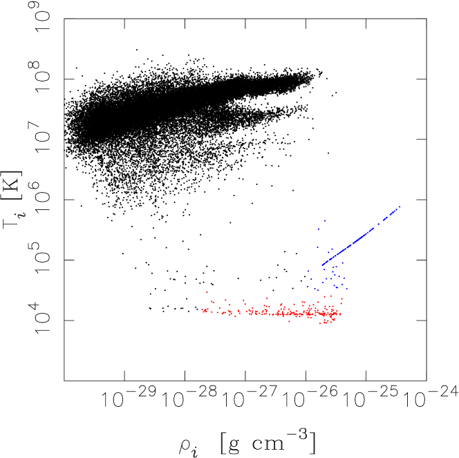
Figure 1.— Scatter plots of temperatures and densities of SPH particles. Red and blue points indicate particles with unphysical temperatures and densities which are removed in computing the X-ray emission.

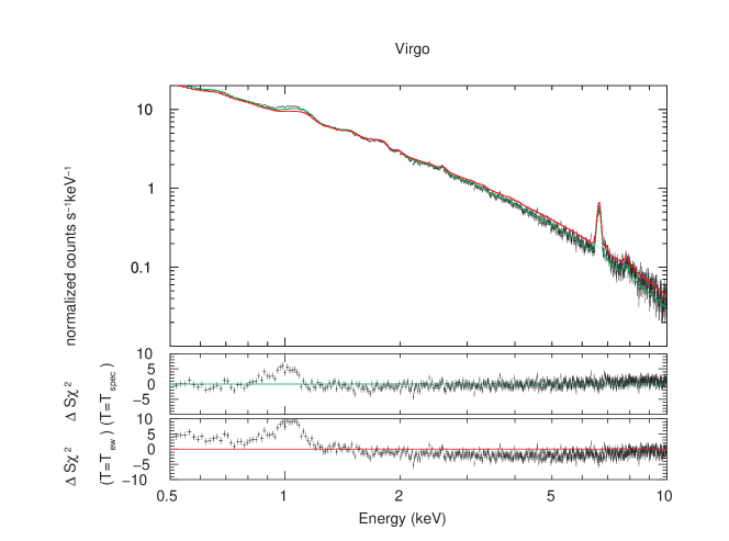
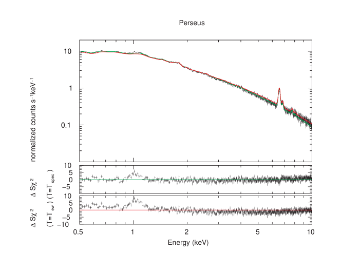
Figure 2.— The examples of the mock spectrum of two simulated clusters. The top panel shows the results for “Virgo” and the bottom panel for “Perseus.” Black marks are the mock spectra. Green line provides the best-fit spectrum, Red line is that of a single temperature thermal model with the temperature $T=T_{\mathrm{ew}}^{\mathrm{sim,m}}$. Each panel has two residuals in terms of sigmas with error bar of size one. Upper one is the residual of the best-fit spectrum ($T=T_{\mathrm{spec}}$). Lower one is that of the thermal model with the emission weighted

temperature ($T=T_{\mathrm{ew}}^{\mathrm{sim,m}}$).

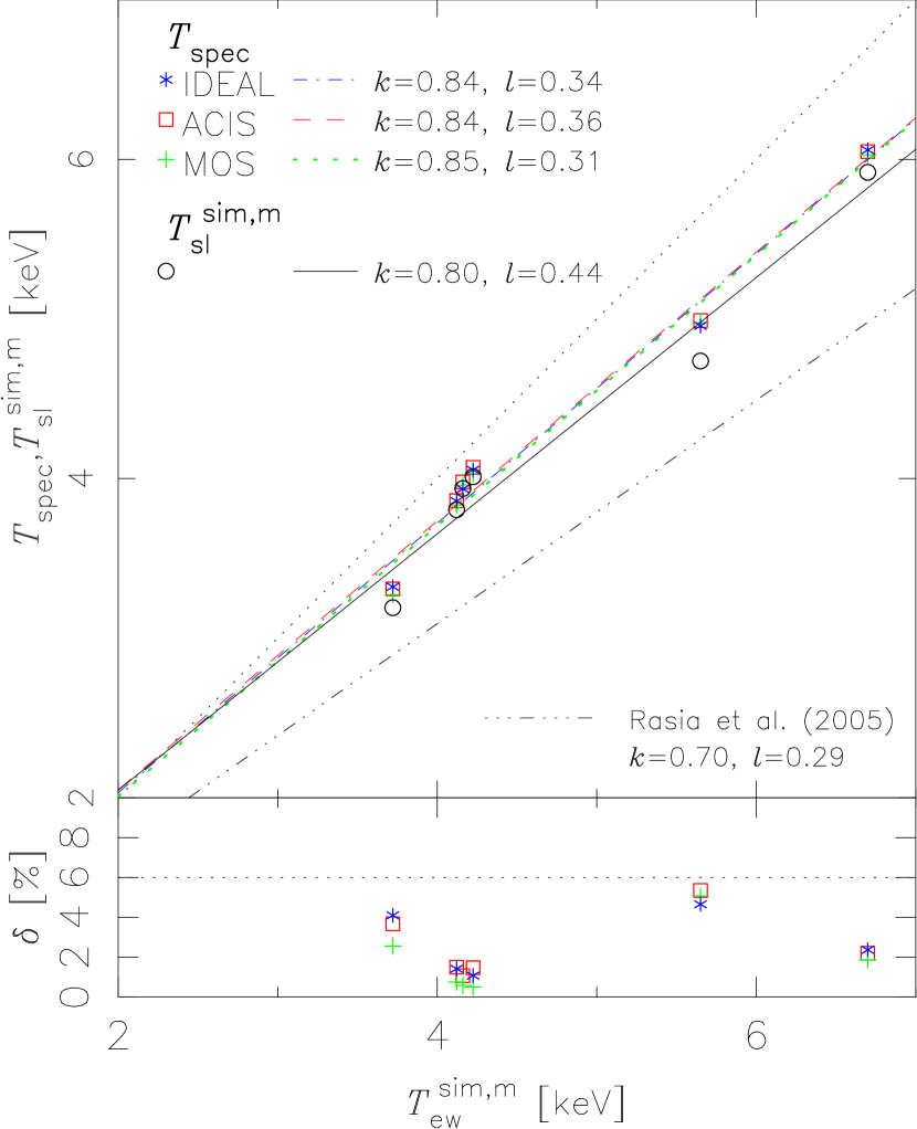
Figure 3.— The upper panel shows the relation of $T_{\mathrm{ew}}^{\mathrm{sim,m}}$ to $T_{\mathrm{spec}}$ (asterisk shows IDEAL, square ACIS, and plus MOS) and $T_{\mathrm{sl}}^{\mathrm{sim,m}}$ (open circle). The lower panel shows the difference between $T_{\mathrm{spec}}$ and $T_{\mathrm{sl}}^{\mathrm{sim,m}}$: $\delta\equiv 100(T_{\mathrm{spec}}/T_{\mathrm{sl}}^{\mathrm{sim,m}}-1)[\%]$, where $T_{\mathrm{spec}}$ is the best-fit temperature of the mock spectra and $T_{\mathrm{sl}}^{\mathrm{sim,m}}$ is given by equation (11).

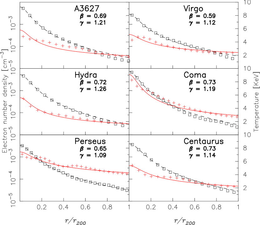
Figure 4.— The radial profile of simulated clusters. Square provides the (electron number) density profile and dashed line is its fitting line assuming the beta model. Plus shows the temperature profile and solid line is its fitting line assuming the polytropic model. Each square and plus point corresponds to the shell with a width of $67h^{-1}~{}\mathrm{kpc}$.

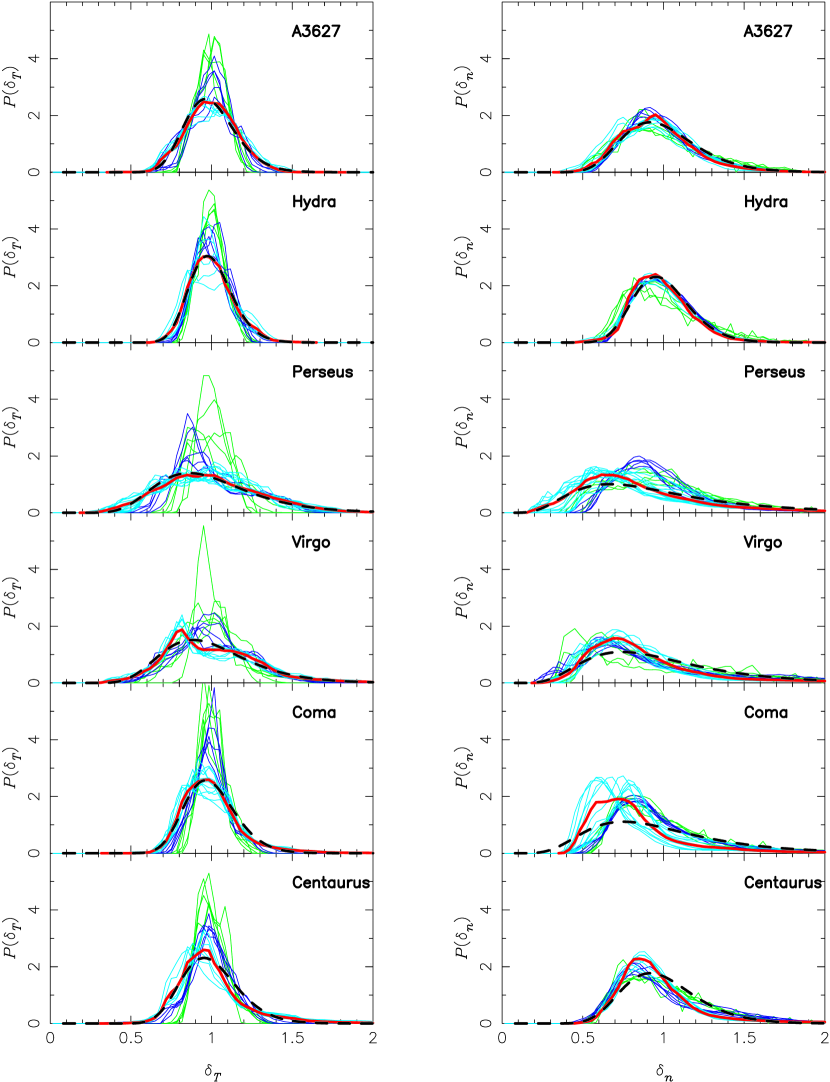
Figure 5.— The distribution of $\delta_{T}\equiv T/\langle T\rangle$ and $\delta_{n}\equiv n/\langle n\rangle$. Thick solid lines present the distribution throughout the mesh points of within $r=r_{200}$. Dashed lines are fitting lines of the log-normal distribution. Thin solid lines are the distribution of the shells each $67h^{-1}~{}\mathrm{kpc}$ distance from the center. Each color indicates different radial interval: $r<335h^{-1}~{}\mathrm{kpc}$ (green), $335h^{-1}~{}\mathrm{kpc}<r<670h^{-1}~{}\mathrm{kpc}$ (blue), and $r>675h^{-1}~{}\mathrm{kpc}$ (cyan).

Figure 6.— The shape of $\kappa^{\mathrm{LI}}(\sigma_{\mathrm{LN},\,T})$ adopting $a=0.75$. In the case of $\sigma_{\mathrm{LN},\,T}=0.1$ and $0.3$, $\kappa^{\mathrm{LI}}\sim 0.99$ and $0.89$, respectively (See Table 1).

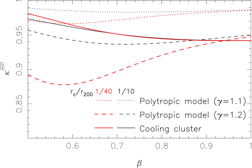
Figure 7.— The bias due to the radial profile $\kappa^{\mathrm{RP}}$ (eq.[31]) assuming the beta model and two temperature models. We assume that the density profile is given by the beta-model. We consider three temperature models: the polytropic model (dotted line provides $\gamma=1.1$, dashed line $\gamma=1.2$) and the cooling cluster model (solid line). We assume the two case of $r_{c}/r_{200}$. One is $r_{c}/r_{200}=1/10$ (black line). Another is $r_{c}/r_{200}=1/40$ (red line).

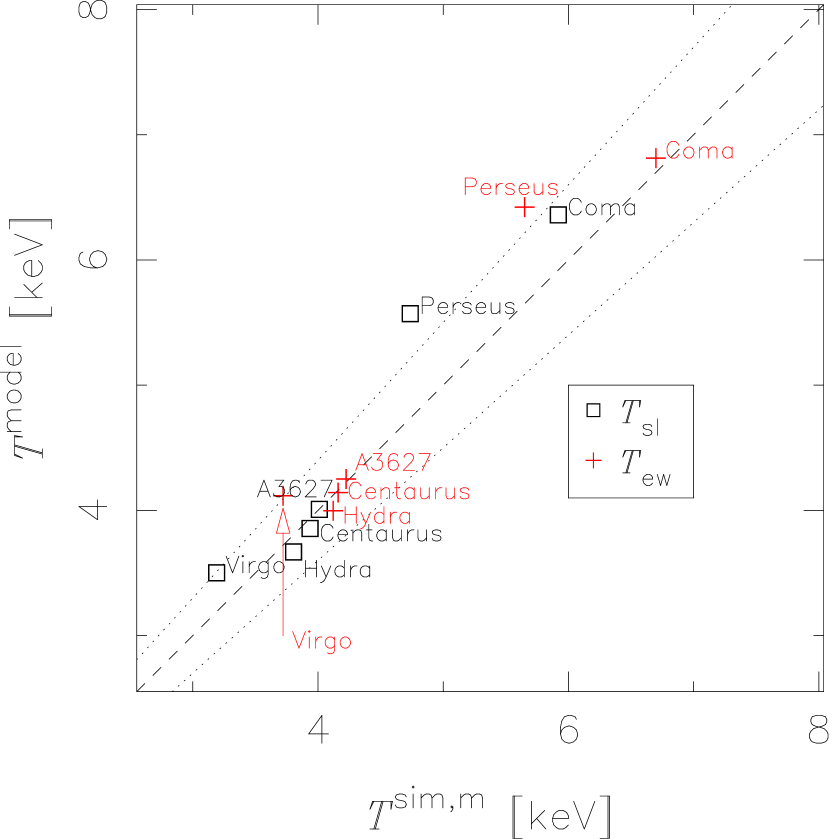
Figure 8.— The emission weighted and spectroscopic like temperature provided our model and the simulation. Dashed line shows $T_{\mathrm{ew}}^{\mathrm{sim,m}}=T_{\mathrm{ew}}^{\mathrm{model}}$ or $T_{\mathrm{sl}}^{\mathrm{sim,m}}=T_{\mathrm{sl}}^{\mathrm{model}}$.Dotted lines show $T_{\mathrm{ew}}^{\mathrm{sim,m}}/T_{\mathrm{ew}}^{\mathrm{model}}-1=\pm 0.1$ or $T_{\mathrm{sl}}^{\mathrm{sim,m}}/T_{\mathrm{sl}}^{\mathrm{model}}-1=\pm 0.1$. In all clusters except “Perseus”, the temperatures of the model reproduce that of the simulation within 10 percent.

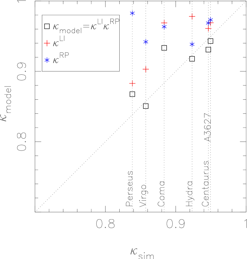
Figure 9.— The bias factor $\kappa$ provided our model and the simulation. Squares show $\kappa_{\mathrm{model}}$. Asterisks and crosses show $\kappa^{\mathrm{RP}}$ and $\kappa^{\mathrm{LI}}$ which are calculated from our model. In all cases, $\kappa_{\mathrm{model}}$ is kept within $\sim 10$ %.

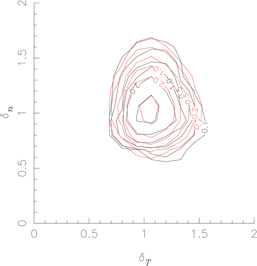
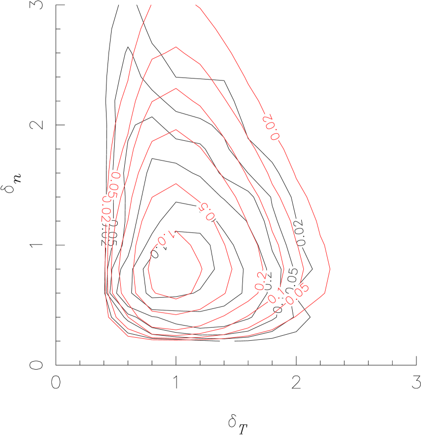
Figure 10.— The contour map of the joint probability P($\delta_{T}$,$\delta_{n}$) within $r_{200}$ (black contour). Red contour indicates the theoretical line of P($\delta_{T}$)P($\delta_{n}$). Left panel shows the case of “Hydra”,Right panel ”Perseus”.

Table 1Properties of the six simulated clusters and observed clusters.

			Simulation
	A3627	Hydra	Perseus	Virgo	Coma	Centaurus
$M_{200}[10^{14}h^{-1}M_{\odot}]$	2.2	1.8	6.7	3.1	4.3	2.5
$r_{200}$ [$h^{-1}$ Mpc]	1.1	1.0	1.6	1.2	1.4	1.1
$\beta$	0.69	0.72	0.65	0.59	0.73	0.73
$\gamma$	1.21	1.26	1.09	1.12	1.19	1.14
$T_{\mathrm{ew}}$ [keV]	4.2	4.1	5.7	3.7	6.7	4.2
$T_{\mathrm{sl}}$ [keV]	4.0	3.8	4.7	3.2	5.9	3.9
$T_{\mathrm{spec}}$ (IDEAL) [keV] (0.5-10.0 keV)	4.1	3.9	5.0	3.3	6.1	3.9
$T_{\mathrm{spec}}$ (ACIS) [keV] (0.5-10.0 keV)	4.1	3.9	5.0	3.3	6.0	4.0
$T_{\mathrm{spec}}$ (MOS) [keV] (0.5-10.0 keV)	4.0	3.8	5.0	3.3	6.0	4.0
$T_{\mathrm{spec}}$ (IDEAL) [keV] (0.1-2.4 keV)	4.0	3.7	4.7	3.1	5.9	3.9
$T_{\mathrm{spec}}$ (IDEAL) [keV] (2.0-10.0 keV)	4.1	4.0	5.4	3.6	6.5	4.0
$\kappa_{\mathrm{sim}}$ (mesh-wise)	0.95	0.92	0.84	0.86	0.88	0.95
$\kappa_{\mathrm{sim}}$ (particle-wise)	0.88	0.89	0.70	0.75	0.84	0.86
$\kappa^{\mathrm{RP}}$	0.97	0.94	0.98	0.94	0.96	0.97
$\sigma_{\mathrm{LN},\,T}$	0.159	0.180	0.316	0.286	0.159	0.178
$\sigma_{\mathrm{LN},\,n}$	0.240	0.180	0.518	0.446	0.434	0.239

			Observation
	A3627	Hydra	Perseus	Virgo	Coma	Centaurus	Ref
$M_{200}[10^{14}h^{-1}M_{\odot}]$	${}^{*}4.6^{+0.81}_{-0.58}$	$1.90^{+0.38}_{-0.33}$	$9.08^{+2.13}_{-1.52}$	$2.04^{+0.28}_{-0.21}$	$4.97^{+0.68}_{-0.57}$	$6.97^{+1.22}_{-1.25}$	1,∗2
$r_{200}$ [$h^{-1}$ Mpc]	∗1.26	1.22	2.05	1.26	1.64	0.89	1,∗2
$T_{\mathrm{spec}}$ [keV]	$5.62^{+0.12}_{-0.11}$	$3.82^{+0.20}_{-0.17}$	$6.42^{+0.06}_{-0.06}$	†$2.5^{+0.04}_{-0.05}$	$8.07^{+0.29}_{-0.27}$	$3.69^{+0.05}_{-0.04}$	3,†4
$N_{\mathrm{H}}$ [$10^{20}\mathrm{cm^{-2}}$]	21.7	4.79	13.9	2.58	0.93	8.1	5
References.–(1)Girardi et al. (1998);(2)Reiprich & Böhringer (2002);(3)Ikebe et al. (2002) (4)Shibata et al. (2001);(5)Dickey & Lockman (1990)

References

- Allen, Schmidt & Fabian (2001) Allen, S. W.; Schmidt, R. W.; Fabian, A. C. 2001, MNRAS, 328, L37
- Borgani et al. (2004) Borgani, S.,Murante, G., Springel, V., Diaferio, A., Dolag, K., Moscardini, L., Tormen, G.,Tornatore, L., & Tozzi, P., 2004, MNRAS, 348, 1078
- Coles & Jones (1991) Coles, P., & Jones, B. 1991, MNRAS, 248, 1
- Dickey & Lockman (1990) Dickey, J.M., & Lockman, F.J., 1990, ARA&A. 28, 215
- Dolag et al. (2005) Dolag, K.,Hansen, F. K.,Roncarelli, & M.,Moscardini, L. 2005, MNRAS, 363, 29
- Girardi et al. (1998) Girardi, M., Giuricin, G., Mardironssian, F., Mezzetti, M., & Boschin, W. 1998, ApJ, 505, 74
- Hubble (1934) Hubble, E. P. 1934, ApJ, 79, 8
- Ikebe et al. (2002) Ikebe, Y., Reiprich, T. H., Böhringer, H., Tanaka, Y., & Kitayama, T. 2002, A&A, 383, 773
- Inagaki, Suginohara & Suto (1995) Inagaki, Y., Suginohara, T., & Suto, Y. 1995, PASJ, 47, 411
- Jing & Suto (2002) Jing, Y. P., & Suto, Y. 2002, ApJ, 574, 538
- Kaastra et al. (2004) Kaastra, J. S., et al. 2004, A&A, 413, 415
- Kasun & Evrard (2005) Kasun, S.F., Evrard, A.E. 2005, ApJ, 629, 781
- Kayo, Taruya & Suto (2001) Kayo, I., Taruya, A., & Suto, Y. 2001, ApJ, 561, 22
- Komatsu et al. (1999) Komatsu, E., Kitayama, T., Suto, Y., Hattori, M., Kawabe, R., Matsuo, H., Schindler, S., & Yoshikawa, K. 1999, ApJ, 516, L1
- Komatsu et al. (2001) Komatsu, E., Matsuo, H., Kitayama, T., Hattori, M., Kawabe, R., Kohno, K., Kuno, N., Schindler, S., Suto, Y., & Yoshikawa, K. 2001, PASJ, 53, 57
- Kitayama et al. (2004) Kitayama, T., Komatsu, E., Ota, N., Kuwabara, T., Suto, Y., Yoshikawa, K., Hattori, M., & Matsuo, H. 2004, PASJ, 56, 17
- Lee, Jing & Suto (2005) Lee, J., Jing. Y.P., & Suto, Y. 2005, ApJ, 632, 706
- Lee & Shandarin (1998) Lee, J. & Shandarin, S.F. 1998, ApJ, 500, 14
- Lee & Suto (2003) Lee, J. & Suto, Y. 2003, ApJ, 585, 151
- Lee & Suto (2004) Lee, J. & Suto, Y. 2004, ApJ, 601, 599
- Makino, Sasaki & Suto (1998) Makino, N., Sasaki, S., & Suto, Y. 1998, ApJ, 497, 555
- Mazzotta et al. (2004) Mazzotta, P., Rasia, E., Moscardini, L., & Tormen, G. 2004, MNRAS, 354, 10
- Mathiesen & Evrard (2001) Mathiesen, B. F., & Evrard, A. E. 2001, ApJ, 546, 1
- Mathis et al. (2002) Mathis, H., Lemson, G., Springel, V., Kauffmann, G., White, S. D. M., Eldar, A., & Dekel, A. 2002,MNRAS, 333, 739
- Morrison & McCammon (1983) Morrison R. & McCammon D., 1983, ApJ, 270, 119
- Nagai, Vikhlinin, & Kravtsov (2006) Nagai, D., Vikhlinin, A., & Kravtsov, A. V. 2006, astro-ph/0609247
- Navarro, Frenk, & White (1997) Navarro, J. F., Frenk, C. S., & White, S. D. M. 1996, ApJ, 462, 563
- Rasia et al. (2005) Rasia, E., Mazzotta, P., Borgani, S., Moscardini, L., Dolag, K., Tormen, G., Diaferio, A., & Murante, G. 2005, ApJ, 618, L1
- Reiprich & Böhringer (2002) Reiprich, T. H., & Böhringer, H., 2002, ApJ, 567, 716
- Salpeter (1955) Salpeter, E. E. 1955, ApJ, 121, 161
- Sheth & Tormen (1999) Sheth, R., & Tormen, G. 1999, MNRAS, 308, 119
- Shibata et al. (2001) Shibata, R., Matsushita, K., Yamasaki, N.Y., Ohashi, T., Ishida, M., Kikuchi, K., Böhringer, H., & Matsumoto, H. 2001, ApJ. 549. 228
- Shimizu et al. (2006) Shimizu, M., Kitayama, T., Sasaki, S., & Suto, Y. 2006, PASJ, 58, 291.
- Springel (2005) Springel, V. 2005, MNRAS, 364, 1105
- Springel et al. (2001) Springel, V., Yoshida, N., & White, S.D.M. 2001,New Astronomy,6,79
- Springel & Hernquist (2002) Springel, V., & Hernquist, L. 2002, MNRAS, 333, 649
- Springel & Hernquist (2003) Springel, V., & Hernquist, L. 2003, MNRAS, 339, 289
- Suto, Sasaki, & Makino (1998) Suto, Y., Sasaki, S., & Makino, N. 1998, ApJ, 509, 544
- Taruya et al. (2002) Taruya, A., Takada, M., Hamana, T., Kayo, I. & Futamase, T. 2002, ApJ, 571, 638
- Tornatore et al. (2004) Tornatore, L., Borgani, S., Matteucci, F., Recchi, S., & Tozzi, P. 2004, MNRAS, 349, L19
- Vikhlinin (2006) Vikhlinin, A. 2006, ApJ, 640, 710
- Wada & Norman (2001) Wada, K., & Norman, C.A.. 2001, ApJ, 547, 172
- Yoshikawa, Itoh & Suto (1998) Yoshikawa, K., Itoh, M., & Suto, Y. 1998, PASJ, 50, 203
- Yoshikawa & Suto (1999) Yoshikawa, K., & Suto, Y. 1999, ApJ, 513, 549
- Yoshikawa et al. (2001) Yoshikawa, K., Taruya, A., Jing, Y.P., & Suto, Y. 2001, ApJ, 558, 520