The evolution of clusters in the CLEF cosmological simulation: X-ray structural and scaling properties

Abstract

We present results from a study of the X-ray cluster population that forms within the CLEF cosmological hydrodynamics simulation, a large $N$-body/SPH simulation of the $\Lambda$CDM cosmology with radiative cooling, star formation and feedback. With nearly one hundred ($kT>2$ keV) clusters at $z=0$ and sixty at $z=1$, our sample is one of the largest ever drawn from a single simulation and allows us to study variations within the X-ray cluster population both at low and high redshift. The scaled projected temperature and entropy profiles at $z=0$ are in good agreement with recent high-quality observations of cool core clusters, suggesting that the simulation grossly follows the processes that structure the intracluster medium (ICM) in these objects. Cool cores are a ubiquitous phenomenon in the simulation at low and high redshift, regardless of a cluster’s dynamical state. This is at odds with the observations and so suggests there is still a heating mechanism missing from the simulation. The fraction of irregular (major merger) systems, based on an observable measure of substructure within X-ray surface-brightness maps, increases with redshift, but always constitutes a minority population within the simulation. Using a simple, observable measure of the concentration of the ICM, which correlates with the apparent mass deposition rate in the cluster core, we find a large dispersion within regular clusters at low redshift, but this diminishes at higher redshift, where strong cooling-flow systems are absent in our simulation. Consequently, our results predict that the normalisation and scatter of the luminosity–temperature relation should decrease with redshift; if such behaviour turns out to be a correct representation of X-ray cluster evolution, it will have significant consequences for the number of clusters found at high redshift in X-ray flux-limited surveys.

1 Introduction

Clusters of galaxies, occurring at low redshifts ($z<2$), are interesting cosmological objects as they offer a powerful yet independent approach from other methods (such as the cosmic microwave background, at $z\sim 1000$) for constraining cosmological parameters. While several cosmological applications of clusters exist, a particularly appealing method, because of its simplicity, is to measure the variation in the cluster mass function with redshift (e.g. Blanchard & Bartlett 1998; Eke et al. 1998). Since mass is known to be tightly correlated with X-ray observables, particularly temperature (e.g. Finoguenov, Reiprich & Böhringer 2001; Arnaud, Pointecouteau & Pratt 2005; Vikhlinin et al. 2006a), it is straightforward in principle to convert between the two quantities.

Theoretically, such cluster scaling relations were predicted to exist, essentially as a manifestation of the virial theorem, by Kaiser (1986). In the so-called gravitational-heating scenario, the intracluster medium (ICM) was heated by the gravitational collapse and subsequent virialisation of the cluster. X-ray observations of clusters confirmed the existence of these scaling relations (e.g. Edge & Stewart 1991; Fabian et al. 1994 for the X-ray luminosity–temperature relation) though they revealed two complications. Firstly, the slope of the observed X-ray luminosity–temperature relation (and to a lesser extent, the mass–temperature relation) is steeper than predicted from gravitational heating alone, an effect shown by Ponman, Cannon & Navarro (1999) to be due to an excess of entropy in the cores of clusters, and more so in groups. A lot of theoretical effort has gone into understanding the origin of the excess entropy (see Voit 2005 for a recent review). Secondly, there is an intrinsic scatter in the scaling relations, which is particularly large for the low-redshift luminosity–temperature relation, due to the large variations in core luminosity (Fabian et al., 1994). For cosmological studies with clusters, an accurate statistical description of the cluster population is warranted, as only then can robust cluster survey selection functions be constructed. From a theoretical stand-point, cluster scaling relations offer an additional, exciting prospect; the amount with which these relations evolve with redshift ought to reveal information on the nature of non-gravitational processes and cluster astrophysics in general (Muanwong, Kay & Thomas, 2006).

The intrinsic scatter in cluster scaling relations can at least partly be attributed to gravitational processes, as clusters themselves live in different environments (e.g. Schuecker et al. 2001), although non-gravitational processes, such as radiative cooling and heating from galaxies, must also play a role (e.g. Pearce et al. 2000; McCarthy et al. 2004; Balogh et al. 2006). Cosmological simulations of the cluster population are the most accurate method by which to characterise the statistical properties of clusters, as they include an accurate treatment of the non-linear gravitational dynamics and merging processes, as well as allowing non-gravitational physics to be incorporated self-consistently. Early attempts focused on the simplest model for the gas, a non-radiative ICM, which was successfully shown to reproduce the simple, self-similar, scalings expected from the gravitational-heating model (e.g. Navarro, Frenk & White 1995; Evrard, Metzler & Navarro 1996; Bryan & Norman 1998; Eke, Navarro & Frenk 1998; Muanwong et al. 2002).

Additional non-gravitational processes have also been studied within simulations, and various mechanisms have been proposed to explain the similarity breaking, such as preheating (e.g. Navarro, Frenk & White 1995; Bialek, Evrard & Mohr 2001; Borgani et al. 2002), radiative cooling (e.g. Pearce et al. 2000; Muanwong et al. 2001, 2002; Davé, Katz & Weinberg 2002; Motl et al. 2004; Kravtsov, Nagai & Vikhlinin 2005) or both (e.g. Muanwong et al. 2002). Recently, attention has shifted to more realistic models which attempt to directly couple feedback (local heating from galaxies) with cooling and star formation (e.g. Valdarnini 2003; Tornatore et al. 2003; Kay, Thomas & Theuns 2003; Borgani et al. 2004; Kay 2004; Kay et al. 2004; Ettori et al. 2004).

Together with progress in the development of these non-gravitational models, the advance in both simulation codes and computer hardware is now allowing larger simulations with reasonable resolution to be performed. We are now beginning to resolve sufficient numbers of clusters to start making quantitative predictions at all appropriate redshifts for the cluster population. The CLEF-SSH (CLuster Evolution and Formation in Supercomputer Simulations with Hydrodynamics) collaboration has been set up to take advantage of this new era in numerical modelling, by performing large simulations of the cluster population. Our first simulation, known as the CLEF simulation, is a large ($N=2\times 428^{3}$) $N$-body/SPH simulation of the $\Lambda$CDM cosmology, within a $200\,h^{-1}\hbox{Mpc}$ box, and includes a model for radiative cooling and energy feedback from galaxies. This simulation is a similar size to the one performed by Borgani et al. (2004), but uses a different feedback model. In Kay et al. (2005), hereafter Paper I, we presented a small selection of results at $z=0$ from the CLEF simulation. For this paper, we have performed a more detailed analysis of the same cluster population, and present results for a range of redshifts from $z=0$ to 1, focusing on the effects of dynamical activity and the strength of cooling cores. A companion paper (da Silva et al., in preparation) presents results for the Sunyaev–Zel’dovich effect properties of the CLEF cluster population.

The rest of this paper is organised as follows. In Section 2 we summarise details of the CLEF simulation and detail our method for creating cluster catalogues, maps and profiles. The internal structure of clusters, and how it depends on dynamical regularity and the properties of the core, is the focus of Section 3. Section 4 then draws on these results to investigate the evolution of key cluster scaling relations with redshift. We discuss our results in Section 5 and summarise our conclusions in Section 6.

2 The CLEF simulation

The CLEF simulation is a large ($N=2\times 428^{3}$ particles within a $200\,h^{-1}\hbox{Mpc}$ comoving box) cosmological simulation of structure formation, incorporating both dark matter and gas. Below we describe the procedure used to generate the simulation data and how the clusters were identified within these data to create X-ray temperature-limited samples from redshifts $z=0$ to $z=1$.

2.1 Simulation details

For the cosmological model, we adopted the spatially-flat $\Lambda$CDM cosmology, setting the following values for cosmological parameters: matter density parameter, $\Omega_{\rm m}=0.3$; cosmological constant, $\Omega_{\Lambda}=\Lambda/3H_{0}^{2}=0.7$; baryon density parameter, $\Omega_{\rm b}=0.0486$; Hubble constant, $h=H_{0}/100\hbox{kms}^{-1}\hbox{Mpc}^{-1}\,=0.7$; primordial power spectrum index, $n=1$ and power spectrum normalisation, $\sigma_{8}=0.9$. These values were chosen to be consistent with the results from WMAP first year data (Spergel et al., 2003).

Initial conditions were generated for a cube of comoving length $200\,h^{-1}\hbox{Mpc}$ at redshift, $z=49$. The cube was populated with two interleaving grids of $428^{3}$ particles, one grid representing the dark matter and one representing the gas; the particle masses were thus set to $m_{\rm dark}=7.1\times 10^{9}\,h^{-1}\hbox{M}_{\odot}$ and $m_{\rm gas}=1.4\times 10^{9}\,h^{-1}\hbox{M}_{\odot}$ for the dark matter and gas respectively. Initial particle displacements and velocities were then computed from a transfer function generated using the CMBFAST code (Seljak & Zaldarriaga, 1996). The initial temperature of the gas was set to $T=100$ K, significantly lower than the range of temperatures typical of overdense structures resolved by the simulation.

The initial conditions were evolved to $z=0$ using a version of the GADGET2 $N$-body/SPH code (Springel, 2006), modified to include additional physical processes (radiative cooling, star formation and energy feedback; see below). Gravitational forces were calculated using the Particle-Mesh algorithm on large scales (using a $512^{3}$ FFT) and the hierarchical tree method on small scales. The (equivalent) Plummer softening length was set to $\epsilon=20\,h^{-1}\hbox{kpc}$, fixed in comoving co-ordinates, thus softening the Newtonian force law below a comoving separation, $x_{\rm min}=2.8\,\epsilon=56\,h^{-1}\hbox{kpc}$.

Gas particles were additionally subjected to adiabatic forces, and an artificial viscosity where the flow was convergent, using the entropy-conserving version of SPH (Springel & Hernquist, 2002), the default method in GADGET2. Additionally, we allowed gas particles with $T>10^{4}$K to cool radiatively, using the isochoric cooling approximation suggested by Thomas & Couchman (1992). Tabulated cooling rates were taken from Sutherland & Dopita (1993), assuming an optically thin $Z=0.3\,\hbox{Z}_{\odot}$ plasma in collisional ionisation equilibrium (a good approximation to the intracluster medium out to at least $z=1$; Tozzi et al. 2003).

2.2 Feedback

We have also attempted to follow crudely the large-scale effects of galactic outflows (feedback) in the simulation, to regulate the cooling rate and to inject non-gravitational energy into the gas. We adopted the Strong Feedback model of Kay (2004), hereafter K2004a, as it was shown there to approximately reproduce the observed excess entropy in groups/clusters, both at small and large radii (see also Paper I). We only give a brief summary of the model details here.

First of all, cooled gas is identified with overdensity $\delta>100$, hydrogen density $n_{\rm H}>10^{-3}\,\hbox{cm}^{-3}$, and temperature $T<12,000$K. For each cooled gas particle, a random number, $r$, is drawn from the unit interval and the gas is reheated if $r<f_{\rm heat}$, where $f_{\rm heat}=0.1$ is the reheated mass fraction parameter. Reheated gas is given a fixed amount of entropy, $S_{\rm heat}=1000\,\hbox{keV}\,\hbox{cm}^{2}$, corresponding to a minimum thermal energy of $\sim 17\,$keV at the star-formation density threshold. Such a high thermal energy (compared with typical cluster virial temperatures) means that the reheated gas is supersonic and is thus distributed through viscous interactions and shocks in the ICM. This not only regulates the star-formation rate in the cluster (Balogh et al., 2001), it also prevents significant build-up of low-entropy material in the cluster core (Kay, Thomas & Theuns, 2003; Kay, 2004). Our model could thus be perceived as a crude representation of local accretion-triggered heating by stars and active galactic nuclei (although feedback from the latter does not necessarily have to follow the star-formation rate, as is done here).

Gas particles that are not reheated are instead converted to collisionless star particles. Although the model does not treat star formation (which occurs in regions with much higher gas densities, $n_{\rm H}\mathrel{\hbox to0.0pt{\lower 3.0pt\hbox{$\sim$}\hss}\raise 2.0pt\hbox{$>$}}0.1$) accurately, this premature removal of low-pressure material from the gas phase saves computational effort as these particles generally have the shortest timesteps. Furthermore, it helps to alleviate the difficulty that standard SPH has in resolving the sharp interface between hot and cold phases (Pearce et al., 2000).

2.3 Cluster identification

The CLEF simulation produced a total of 72 snapshots of the particle data, at time intervals optimised for producing mock lightcones (da Silva et al., in preparation). Only the 25 lowest-redshift snapshots are used in this paper, ranging from $z=0$ to 1; at higher redshift the number of clusters becomes prohibitively small. We used these snapshots to produce cluster catalogues (mass, radius and various other properties), maps and profiles.

Catalogues were generated using a similar procedure to that adopted by Muanwong et al. (2002). Briefly, groups of dark matter particles were identified using the friends-of-friends (FoF) algorithm (Davis et al., 1985), setting the dimensionless linking-length to $b=0.1$. Spheres were then grown around the particle in each group with the most negative gravitational potential, until the enclosed mass equalled a critical value

$$M_{\Delta}(<R_{\Delta})={4\over 3}\pi R_{\Delta}^{3}\,\Delta\,\rho_{\rm cr}(z),$$ (1)

where $\Delta$ is the density contrast, $\rho_{\rm cr}(z)=(3H_{0}^{2}/8\pi G)E(z)^{2}$ is the critical density and $E(z)^{2}=\Omega_{\rm m}(1+z)^{3}+1-\Omega_{\rm m}$ for a flat universe (Bryan & Norman, 1998). Cluster catalogues for a variety of density contrasts were constructed, including the virial value ($\Delta\sim 100$ at $z=0$), taken from equation (6) in Bryan & Norman (1998). The virial radius was used to find overlapping pairs, and the least massive cluster in each pair was discarded from the catalogues. For nearly all of the results presented in this paper, we use a catalogue with $\Delta=500$, as this is the smallest density contrast typically accessible to current X-ray observations.

We initially selected all clusters with at least 3000 particles within $R_{500}$, corresponding to a lower mass limit of $M_{500}=2.5\times 10^{13}\,h^{-1}\hbox{M}_{\odot}$. This limit is low enough that our temperature-selected sample (below) is comfortably a complete subset of this sample at all redshifts studied. At $z=0$ we have 641 clusters in our mass-limited sample, decreasing to 191 clusters at $z=1$. This is comparable to the numbers found in the simulation performed by Borgani et al. (2004), who also used GADGET2 but with a different prescription for cooling, star formation and feedback than used here.

2.4 Spectroscopic-like temperature

Observational samples of X-ray clusters are usually limited in flux or temperature, where the latter is measured by fitting an isothermal plasma model to the observed spectrum of the cluster X-ray emission. Theoretical models of X-ray clusters commonly use an emission-weighted temperature to estimate the spectral temperature of a cluster. For particle-based simulations, this is done using the formula

$$T={\sum_{i}\,w_{i}T_{i}\over\sum_{i}\,w_{i}},$$ (2)

where $w_{i}=m_{i}n_{i}\Lambda(T_{i},Z)$ is the weight given to each hot ($T_{i}>10^{5}$ K) gas particle $i$, $m_{i}$ its mass, $n_{i}$ its density, $T_{i}$ its temperature and $\Lambda(T_{i},Z)$ the cooling function, usually for emission within the X-ray energy band (e.g. Muanwong et al. 2002; Borgani et al. 2004). In the bremsstrahlung regime $\Lambda\propto T^{1/2}$ and so the hottest, densest particles are given the most weight.

Mazzotta et al. (2004) applied the same method used by observers to measure the spectroscopic temperature of simulated clusters, and found that it was always lower than $T_{\rm ew}$. For the bremsstrahlung regime ($kT>2$ keV), they suggested a more accurate measure, known as the spectroscopic-like temperature, with weight $w_{i}=m_{i}n_{i}T_{i}^{-3/4}$. This estimator gives the coldest, densest particles more weight. We adopt this estimator in this paper (summing over gas particles within $R_{500}$ with $kT_{i}>0.5$ keV, the typical lower energy limit of an X-ray band) to create a temperature-limited ($kT_{\rm sl}>2$ keV) sample of clusters at all redshifts. This reduces the number of clusters to 95 at $z=0$, decreasing to 57 at $z=1$. While this is one of the largest temperature-selected cluster sample drawn from a single simulation, we note that the dynamic range is still quite small. Nearly all clusters have $T_{\rm sl}\sim 2-4$ keV at all redshifts (the median temperature stays approximately constant with redshift at $T_{\rm sl}\sim 2.5$ keV) and our hottest cluster at $z=0$ has $T_{\rm sl}=7.3$ keV.

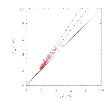
Figure 1: X-ray emission-weighted temperature, $T_{\rm ew}$, plotted against spectroscopic-like temperature, $T_{\rm sl}$, for clusters with $kT_{\rm sl}>2$ keV. The solid line corresponds to $T_{\rm ew}=T_{\rm sl}$ and the dashed line is the best-fit straight line to our data. The dotted line is the best fit to the clusters studied by Rasia et al. (2005).

Fig. 1 compares $T_{\rm sl}$ to $T_{\rm ew}$ (for a $0.5-10$ keV band) for our temperature-limited sample at $z=0$. As was found by Rasia et al. (2005), whose sample mainly consisted of the Borgani et al. (2004) clusters, $T_{\rm sl}$ and $T_{\rm ew}$ differ by as much as 20 per cent. Rasia et al. found $kT_{\rm sl}=0.7kT_{\rm ew}+0.3$, whereas we find $kT_{\rm sl}=0.8kT_{\rm ew}+0.1$, similar to, although slightly steeper than, their result (see also Kawahara et al. 2007).

2.5 Cluster maps and projected profiles

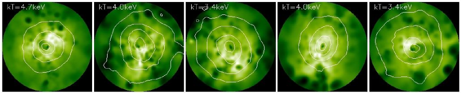
Figure 2: Spectroscopic-like temperature maps of the 5 most massive clusters (in order of decreasing mass, left to right) at $z=1$ (top panels) and $z=0$ (bottom panels). The spectroscopic-like temperature is given in each panel. Surface-brightness contours (normalised to the maximum value) are overlaid; adjacent contours correspond to a difference in surface brightness of a factor of 4. Images are centred on the maximum surface-brightness pixel and are shown out to $R_{500}$.

Cluster maps were produced using a similar procedure to that discussed in Onuora, Kay & Thomas (2003); in essence, values at each pixel are the sum of smoothed contributions from particles, using the same spline kernel as used by the GADGET2 code. Centred on each cluster, only particles within a cube of half-length, $l=4R_{500}$, were considered, i.e. out to approximately twice the virial radius in each orthogonal direction. For this paper, we computed bolometric surface brightness (although the emission is predominantly thermal bremsstrahlung in the X-ray) and spectroscopic-like temperature maps. Projected temperature and azimuthally-averaged surface-brightness profiles were also computed, averaging particles within cylindrical shells, centred on the pixel with the highest surface brightness.

Fig. 2 illustrates spectroscopic-like temperature maps of the 5 most massive clusters each at $z=0$ and $z=1$, out to a radius, $R_{500}$. As was found by Onuora, Kay & Thomas (2003) and Motl et al. (2004), there is a large amount of temperature structure within each cluster, particularly cold spots due to cool, low-entropy gas trapped within infalling sub-clusters. The intensity scale is defined by the minimum and maximum temperature; the dynamic range is typically an order of magnitude ($T_{\rm max}/T_{\rm min}$), with maximum temperatures being around twice that of the mean.

3 Cluster structure

In this section we present the structural properties of the CLEF clusters, comparing to observational data where appropriate.

3.1 X-ray temperature bias

As discussed in the previous section, the X-ray temperature of the ICM is biased to regions of high density. Cooling and heating processes are generally most efficient there, so the X-ray temperature of a cluster is not necessarily an accurate measure of the depth of the underlying gravitational potential well, even if the system is virialised and approximately in hydrostatic equilibrium.

We investigate any such temperature bias in our simulation by comparing $T_{\rm sl}$ to the dynamical temperature, $T_{\rm dyn}$, through the standard quantity, $\beta_{\rm spec}=T_{\rm dyn}/T_{\rm sl}$. The dynamical temperature,

$$kT_{\rm dyn}={\sum_{i,{\rm gas}}\,m_{i}kT_{i}+\alpha\sum_{i}\,\frac{1}{2}m_{i}v_{i}^{2}\over\sum_{i}\,m_{i}},$$ (3)

where $\alpha=(2/3)\mu m_{\rm H}\sim 6.7\times 10^{-25}\,{\rm g}$, assuming the ratio of specific heats for a monatomic ideal gas, $\gamma=5/3$, and the mean atomic weight of a zero metallicity gas, $\mu m_{\rm H}=10^{-24}$ g. The first sum in the numerator runs over gas particles and the second sum over all particles, of mass $m_{i}$, temperature $T_{i}$ and speed $v_{i}$ in the centre of momentum frame of the cluster.

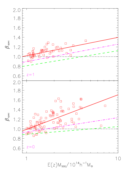
Figure 3: Ratio of dynamical temperature to spectroscopic-like temperature, $\beta_{\rm spec}=T_{\rm dyn}/T_{\rm sl}$, versus scaled mass, $E(z)M_{500}$, at $z=1$ and $z=0$. The solid line is the best-fit relation to the data, while the dot-dashed (dashed) lines are best-fit relations when $T_{\rm sl}$ is replaced by the hot gas mass-weighted temperature excluding (including) bulk kinetic motions.

Fig. 3 illustrates $\beta_{\rm spec}$ for each cluster at $z=1$ and $z=0$, versus its scaled mass, $E(z)M_{500}$. Only clusters with $E(z)M_{500}>10^{14}\,h^{-1}\hbox{M}_{\odot}$ are selected, producing similar numbers to our temperature-selected samples at both redshifts. There is a clear positive correlation between $\beta_{\rm spec}$ and $E(z)M_{500}$, with $\beta_{\rm spec}>1$ for most clusters (i.e. $T_{\rm sl}<T_{\rm dyn}$) at low and high redshift. The spectroscopic-like temperature is a biased tracer of the gravitational potential for three reasons. Firstly, cool dense gas is weighted more than less dense material, as discussed in the previous section. This effect can be seen in the figure by comparing $\beta_{\rm spec}$ to the best-fit relation when $T_{\rm sl}$ is replaced by the hot gas mass-weighted temperature (dot-dashed line). Secondly, some of the energy of the gas is in macroscopic kinetic energy, as can be deduced from comparing the dot-dashed to the dashed line, where in the latter case, $T_{\rm sl}$ is replaced by the temperature when equation (3) is applied to only the hot gas. Finally, feedback heats the gas, particularly in low mass clusters (the dashed line shows that $\beta_{\rm spec}<1$ for most clusters, i.e. the gas has more specific energy than the dark matter).

3.2 Baryon fractions

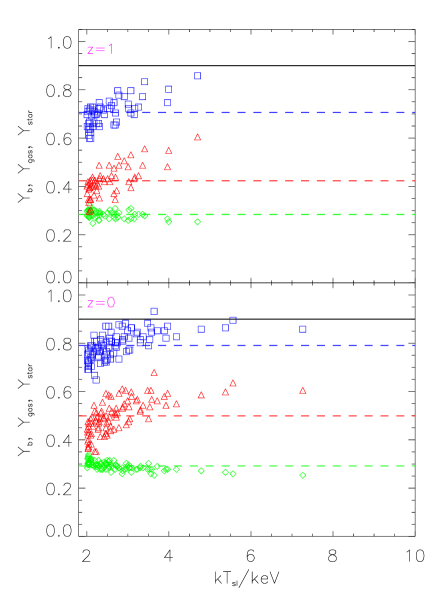
Figure 4: Baryon (squares), gas (triangles) and star (diamonds) fractions versus spectroscopic-like temperature at $z=1$ and $z=0$. Horizontal dashed lines illustrate mean values. The solid line is the average value measured by Kay et al. (2004) for their non-radiative clusters.

We also examine the segregation of baryonic mass into gaseous (ICM) and galactic (collisionless) components within each cluster. Gas and baryon fraction profiles for this model have already been studied by Kay et al. (2004), hereafter K2004b, who showed that the baryon fraction profiles were in good agreement with observations but that too much of the gas had turned into stars (the normalisation of the gas fraction profile is as low as 50 per cent of the observed profile). Here we examine the behaviour of the baryon/gas/star fractions with temperature and redshift.

Fig. 4 illustrates baryon fractions normalised to the global value, $Y_{\rm b}=f_{\rm b}/(\Omega_{\rm b}/\Omega_{\rm m})$ within $R_{500}$, for each cluster at $z=1$ and $z=0$. Most of our clusters have $kT_{\rm sl}<5$ keV, where there is a strong trend in increasing baryon fraction with temperature, as feedback can heat and expel more gas in smaller clusters. At high temperature, a few systems at $z=0$ are consistent with the mean value ($\sim 0.9$) found by K2004b for their non-radiative clusters. Overall, the mean baryon fraction increases by 8 per cent between the two redshifts, from 0.71 at $z=1$ to 0.79 at $z=0$. Similarly, the mean hot gas fraction increases from 0.42 to 0.49 over the same redshift range. Ettori et al. (2004) also found the gas fractions to weakly decrease with redshift in their simulated clusters, albeit with higher values than found here.

The star fraction is a very weak function of both temperature and redshift, with a mean value of 0.28 at $z=0$ and 0.29 at $z=1$. Just under 40 per cent of the baryons within $R_{500}$ have condensed and formed stars in our simulation, at all redshifts; a value that only decreases to about 30 per cent at the virial radius. Observations indicate a value of about 10 to 15 per cent, significantly lower than in our clusters (Lin, Mohr & Stanford, 2003). Thus, as found by K2004b, our feedback model has not been effective enough at limiting the overcooling of baryons in clusters, as was also found by Ettori et al. (2006). However, the global star fraction is only 13 per cent at $z=0$ (and 9 per cent at $z=1$), just slightly larger than the observed value of 5 to 10 per cent (e.g. Balogh et al. 2001).

3.3 Regularity

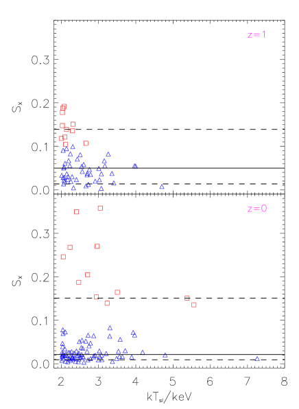
Figure 5: Substructure statistic, $S_{\rm X}$, versus spectroscopic-like temperature for clusters at $z=1$ and $z=0$. Triangles illustrate regular clusters with $S_{\rm X}\leq 0.1$ and squares irregular clusters with $S_{\rm X}>0.1$. The solid horizontal line is the median $S_{\rm X}$ and the dashed lines the 10 and 90 percentiles.

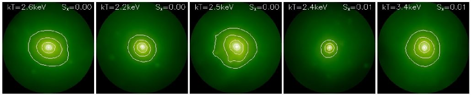
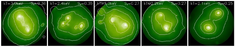
Figure 6: Bolometric surface-brightness maps of the 5 clusters with the lowest (top panels) and 5 with the highest (bottom panels) substructure statistic ($S_{\rm X}$) at $z=0$. In this case, clusters are centred on the surface-brightness centroid.

Hierarchical models of structure formation predict that substructures in clusters should be commonplace, as clusters are the latest result of a series of mergers of smaller systems, and have dynamical times ($\sim 1$ Gyr) that are a significant fraction of the age of the Universe. Indeed, substructure is frequently observed in clusters and dynamical activity has been quantified using various techniques (e.g. Jones & Forman 1992; Mohr, Fabricant & Geller 1993; Buote & Tsai 1995, 1996; Crone, Evrard & Richstone 1996; Schuecker et al. 2001; Jeltema et al. 2005).

We use a simple measure of substructure in our cluster surface-brightness maps, using the centroid-shift method similar to that suggested by Mohr, Fabricant & Geller (1993)

$$S_{\rm X}={|{\bf R}_{\Sigma,{\rm max}}-{\bf R}_{\Sigma,\rm cen}|\over R_{500}},$$ (4)

where ${\bf R}_{\Sigma,{\rm max}}$ is the position of the pixel with maximum surface brightness (taken to be the centre of the cluster) and ${\bf R}_{\Sigma,\rm cen}$ is the surface-brightness centroid. Thomas et al. (1998) used a similar method, based on the 3D total mass distribution, and showed that this did as well, or better, than other more sophisticated measures of substructure in simulated clusters.

Fig. 5 illustrates $S_{\rm X}$ versus $T_{\rm sl}$ for our temperature-limited sample of clusters at $z=1$ (top panel) and $z=0$ (bottom panel). It is evident that the range of $S_{\rm X}$ values at fixed temperature is large: the 10 and 90 percentiles of each distribution, shown as horizontal dashed lines, vary from $\sim 0.01$ to $\sim 0.15$. Inspection of surface-brightness maps (see Fig. 6) reveals that clusters with the largest $S_{\rm X}$ appear dynamically disturbed and are therefore undergoing a major merger. We choose to divide our sample into irregular clusters with $S_{\rm X}>0.1$ and regular clusters otherwise. We note that this division is somewhat arbitrary and only serves to provide us with a means to compare the most disturbed clusters at each redshift to the rest of the sample. The longer tail in the $S_{\rm X}$ distribution to high values at $z=0$ exacerbates the difference between the two sub-populations relative to those at $z=1$ (the length of the tail itself changes from redshift to redshift).

There is no significant trend in $S_{\rm X}$ with temperature, within the limited dynamic range of our sample. However, there is a trend in $S_{\rm X}$ with redshift: the median value at $z=1$ is almost a factor of 2 higher than at $z=0$. In other words, clusters tend to be less regular at higher redshift.

The increase in dynamical activity with redshift in our simulated cluster population is qualitatively consistent with the recent result of Jeltema et al. (2005), who used the more complex power ratios (Buote & Tsai, 1995) to measure dynamical activity in a sample of low- and high-redshift clusters observed with Chandra.

3.4 Temperature and surface-brightness profiles

Surface-brightness and projected temperature profiles are now regularly observed for low-redshift clusters with XMM-Newton and Chandra (e.g. Arnaud, Pointecouteau & Pratt 2005; Vikhlinin et al. 2005; Piffaretti et al. 2005; Zhang et al. 2006; Pratt et al 2007). These are key observable quantities, as 3D density and temperature information can be extracted from these measurements through deconvolution techniques. This allows the thermodynamics of the ICM to be studied, as well as the total mass distribution to be calculated (assuming hydrostatic equilibrium).

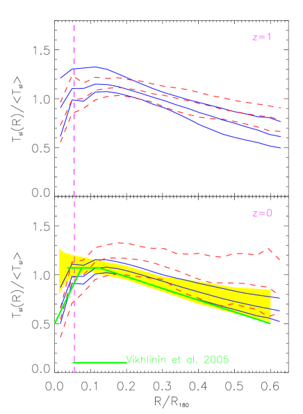
Figure 7: Scaled projected spectroscopic-like temperature profiles at $z=1$ and $z=0$. Solid curves are median and 10/90 percentiles for regular clusters, and dashed curves for irregular clusters. The vertical dashed line illustrates the median scaled softening radius (i.e. where the gravitational force becomes softer than Newtonian). The thick solid lines (with zero and negative gradient) are fits to the average observed temperature profile of cool core clusters, as measured by Vikhlinin et al. (2005); the inner line is a rough fit to their data to illustrate the cool core. The shaded region encloses the mean and $1\sigma$ standard deviation temperature profile for a representative sample of nearby clusters by Pratt et al (2007).

In Fig. 7 we present scaled projected spectroscopic-like temperature profiles for our regular and irregular clusters at $z=1$ and $z=0$. As stated previously, each cluster (including irregular objects, where all emission is included in our analysis) is centred on the pixel with maximum surface brightness. For consistency with the observational data, each temperature profile is normalised to the average spectroscopic-like temperature, $\left<T_{\rm sl}\right>$, between projected radii of $50\,h^{-1}\hbox{kpc}$ and $R_{500}$. Projected radii are then re-scaled to $R_{180}$ using the formula $R_{180}=1.95\sqrt{k\left<T_{\rm sl}\right>/10{\rm keV}}/E(z)\,h^{-1}\hbox{Mpc}$, originally derived from numerical simulations by Evrard, Metzler & Navarro (1996).

As was found by K2004b, the median profile rises sharply from the centre outwards, peaks at $\sim 0.1R_{180}$, then gradually declines at larger radii. The inner rise, where the density is largest, is due to radiative cooling of the gas, while the outer decline is a generic prediction of the $\Lambda$CDM model (e.g. Eke, Navarro & Frenk 1998). It is interesting to note that the shape of the profile for irregular clusters is flatter than for the regular majority, beyond the peak. This is due to the second, infalling, object, which compresses and heats the gas. We also note that the temperature profiles at $z=1$ are very similar to those at $z=0$, and so a cool core is established in the cluster early on.

Vikhlinin et al. (2005) recently determined the projected temperature profile for a sample of 11 low-redshift cool core clusters observed with Chandra. The shape of their profile is very similar, albeit slightly steeper at large radii, to that of our regular clusters; a rough fit, as supplied by the authors, is shown in Fig. 7 as thick solid lines. Pratt et al (2007) performed a similar study with XMM-Newton, for a sample of 15 clusters (including non-cool core systems); their result is shown in the figure as the shaded region. Interestingly, Pratt et al (2007) find a similar decline at large radius to our regular clusters but the temperature does not drop as sharply in the centre (even for those clusters with coolest cores).

The presence of cool cores at both low and high redshift in our simulation is in qualitative agreement with the findings of Bauer et al. (2005), who measured central cooling times for a sample of $z=0.15-0.4$ clusters observed with Chandra and found their distribution to be very similar to that for a local sample.

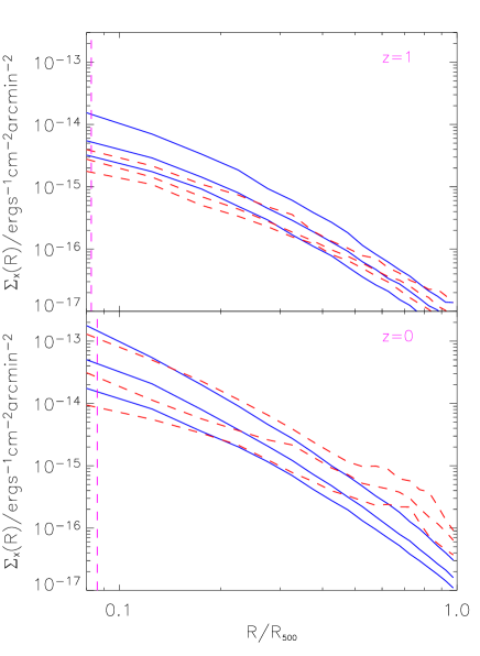
Figure 8: Bolometric surface-brightness profiles at $z=1$ and $z=0$. Again, solid curves are median and 10/90 percentile values for regular clusters, and dashed curves for irregular clusters. The vertical dashed line marks the median force resolution, $\left<2.8\epsilon/R_{500}\right>$.

Bolometric surface-brightness profiles are presented in Fig. 8. At both redshifts, it is clear that there is a larger dispersion between clusters in the core than at the outskirts, particularly at $z=0$. The irregular clusters have flatter profiles than the regular clusters and a bump can be seen at large radius, due to the core of the second object.

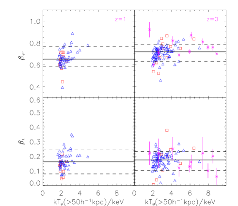
Figure 9: Effective slopes of gas density ($\beta_{\rm eff}$) and temperature ($\beta_{\rm t}$) profiles at $R_{500}$, versus core-excised spectroscopic-like temperature, for clusters at $z=1$ and $z=0$. Triangles are regular clusters and squares irregular clusters. Data points with error bars are from Vikhlinin et al. (2006a).

We also calculate density and temperature gradients for our clusters, as is needed for cluster mass estimates (Section 3.7). Following Vikhlinin et al. (2006a), we define $\beta_{\rm eff}=-(1/3)d\,\ln\rho/d\ln r$ and $\beta_{\rm t}=-(1/3)\,d\ln T/d\ln r$ to represent 3D density and temperature gradients respectively. Fig. 9 shows these values for our clusters at $R_{500}$, plotted against temperature. Results at $z=0$ are overplotted with the Chandra data from Vikhlinin et al. (2006a). In general, the agreement between our results and the observations is very good; median values are $\beta_{\rm eff}=0.76$ and $\beta_{\rm t}=0.19$ respectively. At $z=1$ the median values change very little (0.73 and 0.18).

3.5 Core structure parameters

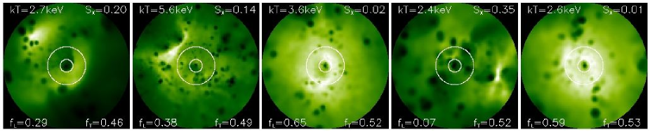
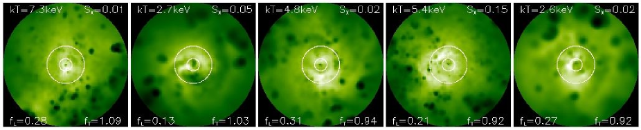
Figure 10: Spectroscopic-like temperature maps of the 5 clusters with the lowest (top panels) and highest (bottom panels) $f_{\rm T}$ values at $z=0$. Circles mark the two inner radii (0.1 and 0.3 $R_{500}$) where $f_{\rm T}$ is measured. X-ray concentrations ($f_{\rm L}$) are also given, which tend to be anti-correlated with $f_{\rm T}$ for regular clusters.

Two generic features of our simulated clusters at $z=0$ is that the majority have cool cores (as shown in Fig. 7) and exhibit a large dispersion in core surface brightness (Fig. 8). At $z=1$, the clusters also tend to have cool cores but a smaller range in core surface brightness is seen. To quantify this behaviour further, we define two simple core structure parameters that are readily observable.

We first define three projected radii, $[R_{1},R_{2},R_{3}]=[0.1,0.3,1.0]R_{500}$. The first approximately defines the radius where the profile stops rising; the first and second approximately define the (maximum) temperature plateau, and the third is the outer radius of the cluster. The first parameter is then

$$f_{\rm T}={T_{\rm sl}(<R_{1})\over T_{\rm sl}(R_{1}\leq R\leq R_{2})},$$ (5)

which measures the ratio of the core to the maximum projected spectroscopic-like temperature of the cluster. Clusters with the coolest cores have the lowest $f_{\rm T}$ values. This can be seen clearly in Fig. 10, where temperature maps of the 5 clusters with the lowest and 5 with the highest $f_{\rm T}$ values are shown. All but two clusters in our sample, including irregular systems, have $f_{\rm T}<1$ because of their cool cores; at $z=1$ the situation is similar, where only 6 clusters ($\sim 10$ per cent of the sample) have $f_{\rm T}>1$ (the median $f_{\rm T}$ increases gradually with redshift). We will return to this point in Section 5.

The second structure parameter is

$$f_{\rm L}={L_{\rm bol}(<R_{1})\over L_{\rm bol}(<R_{3})},$$ (6)

which measures the fraction of bolometric luminosity emanating from the core; we label this the X-ray concentration of the cluster. Clusters with the highest core surface brightness have the highest $f_{\rm L}$ values.

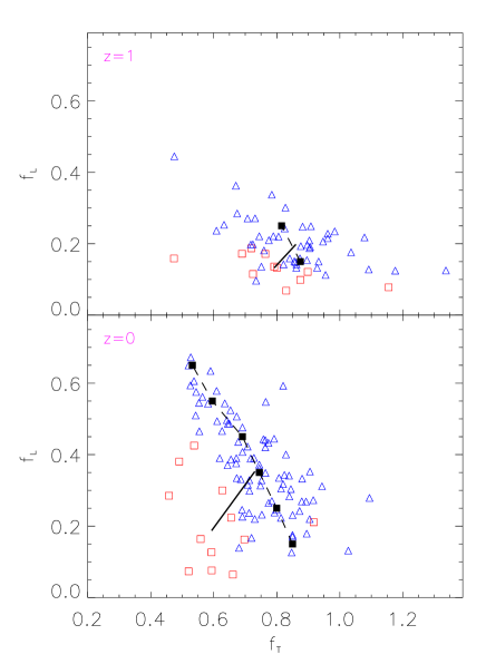
Figure 11: X-ray concentration parameter, $f_{\rm L}$, versus core-to-maximum temperature ratio, $f_{\rm T}$, for clusters at $z=1$ and $z=0$. Triangles are regular clusters and squares irregular clusters, with their median ($f_{\rm T},f_{\rm L}$) co-ordinates connected by a solid line. Solid squares, joined by dashed lines, illustrate the median $f_{\rm T}$ at fixed intervals of 0.1 in $f_{\rm L}$, for regular clusters.

Like $S_{\rm X}$, values of $f_{\rm L}$ and $f_{\rm T}$ do not depend strongly on temperature. Fig. 11 shows that the two quantities are anti-correlated for regular clusters, i.e. clusters with the highest X-ray concentrations have the coolest cores. As we shall see, these systems tend to be older (less recent merger activity), and thus the gas has had more time to settle down into a regular state. Irregular clusters tend to have low $f_{\rm L}$ values as the subcluster boosts the overall luminosity without affecting the core luminosity.

Examining the $f_{\rm L}$ distribution alone, there is a large spread in values at $z=0$, varying from around $0.1-0.7$, but this reduces to $\sim 0.1-0.4$ at $z=1$. As expected from Fig. 8, we see an absence of clusters with strongly-peaked X-ray emission at high redshift (the median $f_{\rm L}$ decreases gradually with redshift). It is unlikely that this effect is due to poorer numerical resolution at higher redshift, as nearly all our clusters have an inner radius, $R_{1}$, that is larger than the physical softening radius, $r_{\rm min}=56\,h^{-1}\hbox{kpc}/(1+z)$, at $z=0$ and $z=1$. Furthermore, the lack of a strong dependence of $f_{\rm L}$ with temperature and the presence of cool cores at all redshifts suggests that numerical heating cannot be a major problem.

3.6 Entropy profiles

The combined effects of cooling and heating processes can be effectively probed by measuring the entropy distribution of the ICM and comparing this with the prediction of the gravitational-heating model (see Voit 2005 and references therein). Recently, Voit, Kay & Bryan (2005) compared two independent sets of gravitational-heating simulations and found that the outer entropy profiles were very similar, $S\propto R^{1.2}$, close to the original prediction from spherical accretion-shock models (e.g. Tozzi & Norman 2001). K2004a and K2004b found that cooling and feedback (the same model used in this paper) only slightly modified the outer slope of the entropy profile; the main effect was an increase in the normalisation of the entropy at all radii, as suggested by observations (e.g. Ponman, Sanderson & Finoguenov 2003; Pratt & Arnaud 2003).

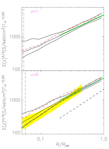
Figure 12: Scaled entropy versus radius, in units of $R_{200}$, for clusters at $z=1$ and $z=0$. The solid curves are the median and 10/90 percentile profiles for regular clusters, the dashed curve is the median profile for irregular clusters and the dot-dashed curve for regular clusters with $f_{\rm L}>0.45$. The vertical dashed line illustrates the force resolution of the simulation. The large shaded region encloses the mean and $1\sigma$ standard deviation entropy profile for an observed sample of clusters by Pratt, Arnaud & Pointecouteau (2006). A least-squares fit to the simulated data at $R>0.2R_{200}$ is illustrated by the thick solid line, flatter than the prediction from gravitational-heating simulations, $S\propto R^{1.2}$, shown with the lower dashed line (Voit, Kay & Bryan, 2005).

The CLEF simulation allows us to study entropy profiles for a much larger sample of clusters than previously. In Paper I, we showed that the entropy–temperature relation at $z=0$ reproduced the observed behaviour of excess entropy, both at small ($0.1R_{200}$) and large ($R_{500}$) radii. In this paper, we focus on the scaled entropy profiles at $z=0$ and $z=1$, shown in Fig. 12. We scale the entropy profile of each cluster by $E^{4/3}(z)T_{10}^{-0.65}$; the first factor reflects the predicted redshift scaling from gravitational heating, while the second approximately represents the scaling with temperature at fixed radius/overdensity, modified by non-gravitational processes. As will be explained below, we define $T_{10}$ to be the projected spectroscopic-like temperature in $10{\rm keV}/k$ units, measured between $R_{1}$ and $R_{2}$ (i.e. the temperature plateau, see subsection 3.5).

The solid curves illustrate the median and 10/90 percentile profiles for regular clusters at each redshift. At both redshifts the profiles are close to power-law outside the core ($R\sim(0.2-1)R_{200}$); fitting a straight line to the profile in this region yields $S\propto R^{0.9}$ at both redshifts, as found in previous papers (K2004a,b). Note that at $R_{500}$, the normalisation of the scaled profile is very similar at $z=0$ and $z=1$, thus the entropy at large radii scales with redshift as predicted from gravitational-heating models.

We also plot the median profile of irregular clusters (shown as the dashed curve) and at $z=0$, clusters with the highest X-ray concentrations ($f_{\rm L}>0.45$). Irregular clusters tend to have higher entropy profiles than the regular clusters at all radii and at both redshifts. This temporary elevation in entropy reflects the shock-heating processes associated with the merger. Conversely, clusters with the highest X-ray concentrations have the lowest entropy profiles, reflecting the fact that they have the highest cooling rate. We also note that the profile for these systems resembles a broken power law, similar to that observed by Finoguenov, Böhringer & Zhang (2005) in their REFLEX-DXL clusters ($z\sim 0.3$).

We compare the profiles at $z=0$ to the recent XMM-Newton data studied by Pratt, Arnaud & Pointecouteau (2006) (the mean plus/minus $1\sigma$ values are shown as the shaded region). Pratt, Arnaud & Pointecouteau (2006) use a global mean temperature, measured between $0.1-0.5R_{200}$, for the entropy scaling. We note, however, that this effectively measures their temperature plateau as they see no significant evidence of a decline at large radii (Arnaud, Pointecouteau & Pratt, 2005). The simulated (regular clusters) and observed distributions are similar, although the simulated profile is slightly high. We note, however, that our regular, concentrated clusters fit the observational profile very well; the observed sample is probably biased to systems of this type as they are intrinsically brighter systems and are thus easier to observe.

3.7 Mass estimates

Finally in this Section, we briefly investigate the validity of hydrostatic equilibrium in the simulated clusters at all redshifts, used to estimate cluster masses from X-ray data

$$M_{\rm est}(<r)=-{rkT(r)\over G\mu m_{\rm H}}\,\left[{d\ln\rho\over d\ln r}+{d\ln T\over d\ln r}\right],$$ (7)

where $\rho(r)$ and $T(r)$ are the 3D density and spectroscopic-like temperature profiles respectively. Various approximations to equation (7) have been used previously in the literature, when little or no spatial information was available for the temperature distribution in clusters. Newer, high-quality observations with XMM-Newton and Chandra have overcome this problem (e.g. Arnaud, Pointecouteau & Pratt 2005; Vikhlinin et al. 2006a), and so we assume in our study that the gas density and temperature profiles can be accurately recovered from the X-ray data out to $R_{500}$. (A detailed study of obtaining such profiles from mock X-ray data is left to future work, but see Rasia et al. 2006.)

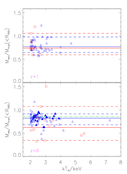
Figure 13: Ratio of estimated to true masses at $R_{500}$ versus $T_{\rm sl}$ for clusters at $z=1$ and $z=0$. Squares are irregular clusters, triangles are regular clusters and filled triangles regular clusters with the highest X-ray concentrations, $f_{\rm L}>0.45$. Solid (dashed) lines are median (10/90 percentile) ratios for regular and irregular clusters. The dot-dashed line is the median ratio for regular clusters with $f_{\rm L}>0.45$.

In Fig. 13, we plot estimated to true mass ratios at $R_{500}$ for our clusters at $z=1$ and $z=0$. For internal consistency, estimated masses are those at the estimated $R_{500}$, which is typically 5 per cent smaller than the true $R_{500}$.

The median estimated mass is around 80 per cent of the true mass at both redshifts for regular clusters, with 10-20 per cent scatter. Irregular clusters tend to have slightly poorer mass estimates on average, but the scatter is also larger. Clusters with the highest X-ray concentrations perform slightly better than the regular clusters as a whole.

Our median mass ratio is lower than found by K2004b at $z=0$, who found that the average estimated mass was only 5 per cent or so lower than the true mass at $R_{500}$, with the small discrepancy being due to turbulent motions (see also Evrard, Metzler & Navarro 1996; Rasia et al. 2004). The reason for the difference is twofold. Firstly, K2004b used a mass-weighted temperature profile, where we use the more realistic spectroscopic-like temperature profile. This reduces mass estimates by 10 per cent or so, similar to what was found by Rasia et al. (2006), when assuming a low X-ray background in their analysis. A further 5 per cent reduction comes from using the estimated $R_{500}$ rather than the true value, which also increases the scatter. While we are therefore not comparing true and estimated masses at the same radius here, we are demonstrating what the overall effect will be on the normalisation of the mass–temperature relation, as will be investigated in the next section.

4 Cluster Scaling Relations

We now put together the results from previous sections to try and understand the properties of cluster scaling relations in our simulation. We consider the two most important X-ray scaling relations in this paper: mass versus temperature ($M-T$) and luminosity versus temperature ($L-T$), with all quantities computed within $R_{500}$.

Scaling relations are defined using the conventional form

$$Y=Y_{0}\,(X/X_{0})^{\alpha}\,(1+z)^{\beta},$$ (8)

where $Y_{0}$ is the normalisation at $X=X_{0}$ and $z=0$ (for all relations, $X_{0}=5{\rm keV}$ ; for the $M-T$ relation, $Y_{0}=M/10^{14}\,h^{-1}\hbox{M}_{\odot}$ and for the $L-T$ relation, $Y_{0}=L/10^{44}h^{-2}{\rm ergs}^{-1}$); $\alpha$ is the slope and $\beta$ the parameter used to describe the redshift dependence of the normalisation. Scatter in the relations is measured at each redshift as

$$\sigma_{\log(Y)}=\sqrt{{1\over N}\,\sum_{i}\,(\log(Y_{i}/Y))^{2}}$$ (9)

i.e. the r.m.s. deviation of $\log(Y)$ from the mean relation, where $Y_{i}$ are individual data points. We then parameterise any redshift dependence of the scatter using a least-squares fit to $\sigma_{\log(Y)}$

$$\left<\sigma_{\log(Y)}\right>(z)=\sigma_{0}+\sigma_{1}\log(1+z).$$ (10)

4.1 Results at $z=0$

Table 1: Best-fit parameter values (and $1\sigma$ errors) for scaling relations at $z=0$. Column 1 gives the sample used in the fit; column 2 the best-fit normalisation; column 3 the best-fit slope and column 4 the logarithmic scatter.

Sample	$Y_{0}$	$\alpha$	$\sigma_{\log(Y)}$
$M_{500}-T_{\rm dyn}$
All	$3.44\pm 0.07$	$1.38\pm 0.03$	$0.05$
Reg	$3.46\pm 0.08$	$1.38\pm 0.04$	$0.05$
High	$3.53\pm 0.11$	$1.38\pm 0.07$	$0.03$
Low	$3.40\pm 0.11$	$1.36\pm 0.05$	$0.05$
$M_{500}-T_{\rm gas}$
All	$4.08\pm 0.06$	$1.69\pm 0.03$	$0.03$
Reg	$4.05\pm 0.06$	$1.67\pm 0.03$	$0.03$
High	$3.95\pm 0.12$	$1.59\pm 0.06$	$0.03$
Low	$4.07\pm 0.08$	$1.69\pm 0.03$	$0.03$
$M_{500}-T_{\rm sl}$
All	$5.51\pm 0.32$	$1.81\pm 0.08$	$0.08$
Reg	$4.93\pm 0.29$	$1.69\pm 0.08$	$0.08$
High	$7.03\pm 0.78$	$1.96\pm 0.16$	$0.06$
Low	$4.37\pm 0.21$	$1.61\pm 0.07$	$0.06$
$M_{500}-T_{\rm sl}^{50}$
All	$4.47\pm 0.19$	$1.76\pm 0.07$	$0.08$
Reg	$4.02\pm 0.12$	$1.64\pm 0.05$	$0.05$
High	$3.94\pm 0.13$	$1.62\pm 0.07$	$0.03$
Low	$4.08\pm 0.17$	$1.66\pm 0.06$	$0.05$
$M_{500}^{\rm est}-T_{\rm sl}^{50}$
All	$3.28\pm 0.15$	$1.64\pm 0.08$	$0.09$
Reg	$3.11\pm 0.11$	$1.57\pm 0.06$	$0.06$
High	$3.22\pm 0.15$	$1.56\pm 0.10$	$0.04$
Low	$2.98\pm 0.15$	$1.53\pm 0.08$	$0.06$
$L_{\rm bol}-T_{\rm sl}$
All	$6.0\pm 1.1$	$3.08\pm 0.26$	0.27
Reg	$5.8\pm 1.3$	$3.04\pm 0.30$	0.27
High	$19.0\pm 6.5$	$3.61\pm 0.45$	0.16
Low	$3.6\pm 0.5$	$2.81\pm 0.19$	0.16
$L_{\rm bol}^{50}-T_{\rm sl}^{50}$
All	$4.3\pm 0.3$	$3.45\pm 0.13$	0.14
Reg	$3.9\pm 0.3$	$3.37\pm 0.12$	0.12
High	$4.7\pm 0.3$	$3.16\pm 0.12$	0.05
Low	$3.1\pm 0.3$	$3.13\pm 0.14$	0.11

Our results for $z=0$ clusters are summarised in Table 1. Column 1 lists the sample used when fitting the data. Here, we consider all 95 clusters in our temperature-limited sample (labelled All), the 83 regular clusters (i.e. those with $S_{\rm X}\leq 0.1$; labelled Reg), the 23 regular clusters with the most prominent core emission ($f_{\rm L}>0.45)$; denoted High) and the 60 remaining regular clusters (denoted Low). Column 2 lists the best-fit normalisation, $Y_{0}$; column 3 the slope of the relation, $\alpha$; and column 4 the scatter in the relation, $\sigma_{\log(Y)}$. We now discuss each relation in turn.

4.1.1 $M_{500}-T$ relation

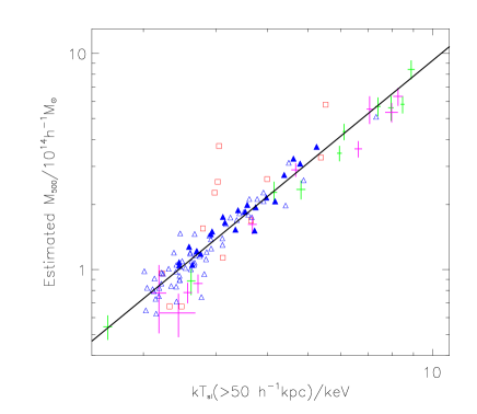
Figure 14: Estimated scaled-mass at $R_{500}$ versus spectroscopic-like temperature outside the core at $z=0$. Squares are irregular clusters, triangles are regular clusters and filled triangles regular clusters with the highest X-ray concentrations, $f_{\rm L}>0.45$. The solid line in each panel is a best fit to regular clusters. Crosses are data-points from Arnaud, Pointecouteau & Pratt (2005) and Vikhlinin et al. (2006a).

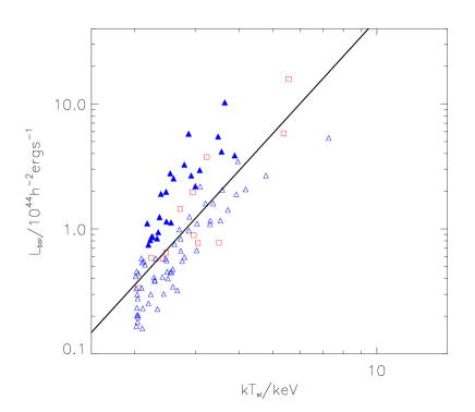
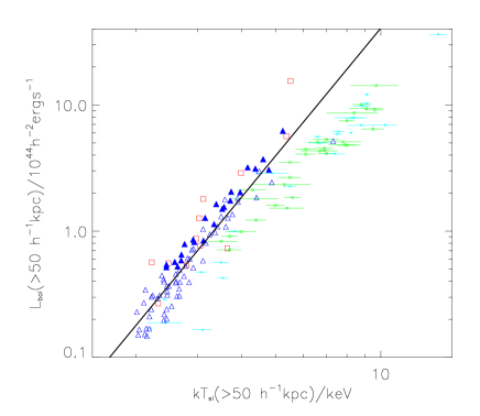
Figure 15: Bolometric luminosity versus spectroscopic-like temperature, for all emission (left panel) and emission outside the core (right panel). Squares are irregular clusters, triangles are regular clusters and filled triangles regular clusters with the highest X-ray concentrations, $f_{\rm L}>0.45$. The solid line in each panel is a best fit to regular clusters. Data points with error bars are observed values from Markevitch (1998) and Arnaud & Evrard (1999).

We first study the $M-T$ relation at $z=0$. In Paper I we presented results for the hot gas mass-weighted temperature within $R_{2500}$, $T_{\rm gas}$, and showed that the relation was in good agreement with the Chandra results of Allen, Schmidt & Fabian (2001). Here we discuss the $M$–$T$ relation at $R_{500}$ as we expect it to be less susceptible to cooling and heating effects associated with the cluster core. While measuring the relation at $R_{500}$ is observationally challenging, even with XMM-Newton and Chandra, recent attempts have been performed for a small sample of clusters with a reasonable range in temperature (Arnaud, Pointecouteau & Pratt 2005, hereafter APP05; Vikhlinin et al. 2006a, hereafter VKF06). We will eventually compare our results at $z=0$ to these observations, but first study how our definition of temperature and mass affects the details of the relation.

We initially consider the relation between the true total mass of a cluster, $M_{500}$, and its dynamical temperature, $T_{\rm dyn}$, where the latter was defined in equation (3). This relation should most faithfully represent the scaling expected from gravitational-heating models ($\alpha=1.5$) but as listed in Table 1, the measured slope is slightly shallower than this ($\alpha\sim 1.4$). As discussed in Muanwong, Kay & Thomas (2006), the deviation in slope is consistent with the variation in halo concentration with cluster mass (i.e. even the dark matter is not perfectly self-similar). Note that the sub-samples give almost identical results to the overall sample, although the High sub-sample exhibits less scatter.

We next consider the hot gas mass-weighted temperature, $T_{\rm gas}$. The slope of the relation steepens to $\alpha\sim 1.7$; as discussed in Section 3.1, this is due to the combined effects of heating and cooling. Strikingly, the scatter in this relation is very small ($\sigma_{\log(T)}=0.03$). Again, no significant change in the relation is observed when the cluster sub-samples are considered.

When the X-ray temperature, $T_{\rm sl}$, is used, both the normalisation and scatter increase, with the irregular and High clusters lying above the mean relation (i.e. they are colder than average). This is because cool, dense gas in the core and in substructures throughout the cluster (see Fig. 2) is weighted more heavily than before, and there is a large variation in the cool gas distribution from cluster to cluster (see also Muanwong, Kay & Thomas 2006; O’Hara et al. 2006). As can be seen in Fig. 11, the irregular and the High clusters have the lowest $f_{\rm T}$ values.

We also present results for the spectroscopic-like temperature when particles from within the inner $50\,h^{-1}\hbox{kpc}$ core are excluded (denoted $T_{\rm sl}^{50}$), which reduces the scatter in the Reg clusters from 0.08 to 0.05. The High and Low relations are now consistent with the overall Reg relation, although the irregular clusters still lie above the relation as a second cool core is still present.

Finally, we replace the actual mass with the mass estimated under the assumption of hydrostatic equilibrium (denoted $M_{500}^{\rm est}$), as defined in Section 3.7. Fig. 14 illustrates the result, in comparison to the data from APP05 and VKF06. The relation for the Reg subsample provides the closest match to the observational data. The main effect of using the estimated mass is to reduce the normalisation by $\sim 20$ per cent. Although the two observational samples are similar, our Reg relation is closest to the best-fit results of VKF06; the slope and scatter are almost identical (VKF06 find $\alpha=1.58$ and $\sigma_{\log(M)}\sim 0.06$) and the normalisation differs by 10 per cent or so (VKF06 find $Y_{0}=2.89\pm 0.15$). Given the variations between parameters considered in this study, this is quite a good match, but serves to point out that a precision measurement of the $M-T$ relation is non-trivial and must include several physical effects; our present study is by no means exhaustive (see Rasia et al. 2006).

4.1.2 $L-T$ relation

To study the luminosity–temperature relation, we compute bolometric luminosities, $L_{\rm bol}$, for all emission within $R_{500}$ (where more than 90 per cent of the cluster emission comes from). We also compute luminosities outside the core (denoted $L_{\rm bol}^{50}$), again by excluding all hot gas particles from within $50\,h^{-1}\hbox{kpc}$ from the cluster’s centre.

Fig. 15 illustrates luminosity–temperature relations at $z=0$. In the left panel we show results for total luminosities and spectroscopic-like temperatures, and in the right panel, for luminosities and temperatures outside the $50\,h^{-1}\hbox{kpc}$ core. Best-fit parameters for the various cluster samples at $z=0$ are also given in Table 1.

When all emission is included, the $L-T$ relation at $z=0$ has a large amount of scatter. Comparing the relation for regular clusters with high $f_{\rm L}$ values to those with low $f_{\rm L}$ values, we see that the two subpopulations are widely separated in the $L-T$ plane. The scatter thus reflects the strength of the core emission, as shown observationally by Fabian et al. (1994). We discuss this further in Section 5.

When the $50\,h^{-1}\hbox{kpc}$ core emission is excised, the scatter in the relation reduces substantially, from 0.27 to 0.14, with all samples then having very similar properties. We also note that irregular clusters do not lie systematically off the $L-T$ relation, in agreement with Rowley, Thomas & Kay (2004), who analysed a simulation with radiative cooling but no feedback.

We compare our excised-core results with the observational data of Markevitch (1998) and Arnaud & Evrard (1999); the former also excised emission from the inner $50\,h^{-1}\hbox{kpc}$ and the latter selected non-cooling-flow clusters. Although our clusters do not cover the same dynamic range as the observations, we note that our $L-T$ relation has a normalisation that is too high (see also Paper I). This suggests that that cluster temperatures in general are too low (note that higher temperatures may not significantly affect the normalisation of the $M-T$ relation, as the estimated mass depends linearly on $T$). The slope of the relation for all clusters, $\alpha=3.5$, is steeper than the observations ($\alpha\sim 2.6-2.9$). As stated in Paper I, the slope varies systematically with temperature, such that higher-mass clusters have lower values. The lack of hot clusters in our sample biases our result to higher values. Significantly larger volumes are still required to capture the rich clusters, to get a more accurate (average) slope for the cluster population.

4.2 Evolution of scaling relations

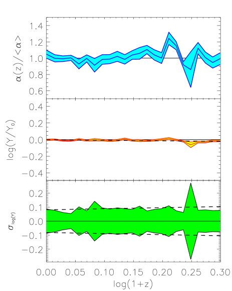
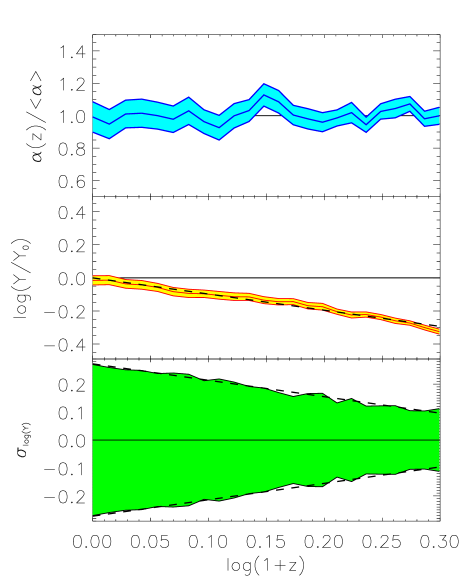
Figure 16: Redshift dependence of the slope, normalisation and scatter of the $M_{500}^{\rm est}-T_{\rm sl}^{50}$ (left panel) and $L_{\rm bol}-T_{\rm sl}$ (right panel) scaling relations. The band in the top panel illustrates the mean slope plus the standard deviation at each redshift, all normalised to the median value over all redshifts between $z=0-1$. The band in the middle panel illustrates the mean and standard deviation of the normalisation at each redshift (assuming a fixed slope, at the median value). The best-fit straight line to the mean data is also plotted as a dashed line and is used to normalise the data at $z=0$. The band in the bottom panel illustrates the logarithmic scatter in the scaling relations at each redshift (values are reflected about the x-axis to give an idea of the full size of scatter in the relation), with the best-fit straight line given by the dashed line.

We now study how the $M-T$ and $L-T$ relations evolve with redshift. We first measure the slope, normalisation and scatter of the relations at each redshift between $z=0$ and $z=1$. The gravitational-heating model predicts the slope to be constant with redshift. For the $M-T$ relations this is generally true; although the variation can be quite noisy, there is no evidence for a systematic change in the slope, $\alpha$, with redshift (e.g. see the top-left panel in Fig. 16 for how the slope changes with redshift in the $M_{500}^{\rm est}-T_{\rm sl}^{50}$ relation). For the $L-T$ relation (all emission), the slope increases with redshift when all clusters are considered. This is because the few hottest clusters have anomalously high temperatures for their luminosity at low redshift, causing a decrease in slope since they carry a lot of weight. At higher redshift the effect diminishes as the clusters move back towards the mean relation. We circumvent this problem by restricting our fit to the $L-T$ relation to clusters with $2<kT<5$ keV at each redshift; as can be seen in the top-right panel of Fig. 16, the slope of the $L_{\rm bol}-T_{\rm sl}$ relation is now approximately constant. For all relations, we fix $\alpha$ to its median value between $z=0-1$.

With $\alpha$ determined, we then fit equation (8) to the normalisation data to determine $Y_{0}$ and $\beta$. (Note this may cause $Y_{0}$ to change slightly from the exact $z=0$ value.) The scatter is also determined at each redshift (equation 9) and fit with equation (10).

Table 2: Best-fit parameter values (and $1\sigma$ errors) for evolution of scaling relations from $z=0-1$. Column 1 gives the median slope used for the fit; columns 2 & 3 the best-fit normalisation and evolution parameters; and columns 4 & 5 the best-fit scatter parameters.

$\left<\alpha\right>$	$Y_{0}$	$\beta$	$\sigma_{0}$	$\sigma_{1}$
$E(z)M_{500}-T_{\rm dyn}$
$1.40$	$3.48\pm 0.02$	$-0.07\pm 0.01$	$0.05\pm 0.002$	$-0.02\pm 0.01$
$E(z)M_{500}-T_{\rm gas}$
$1.68$	$4.08\pm 0.02$	$-0.12\pm 0.01$	$0.04\pm 0.004$	$0.03\pm 0.02$
$E(z)M_{500}-T_{\rm sl}$
$1.77$	$5.21\pm 0.04$	$-0.13\pm 0.02$	$0.08\pm 0.003$	$-0.05\pm 0.01$
$E(z)M_{500}-T_{\rm sl}^{50}$
$1.67$	$4.24\pm 0.03$	$0.04\pm 0.02$	$0.07\pm 0.003$	$-0.03\pm 0.02$
$E(z)M_{500}^{\rm est}-T_{\rm sl}^{50}$
$1.56$	$3.17\pm 0.04$	$-0.07\pm 0.03$	$0.08\pm 0.02$	$0.08\pm 0.10$
$E^{-1}(z)L_{\rm bol}-T_{\rm sl}$
$3.36$	$7.36\pm 0.09$	$-0.98\pm 0.03$	$0.27\pm 0.003$	$-0.59\pm 0.02$
$E^{-1}(z)L_{\rm bol}^{50}-T_{\rm sl}^{50}$
$3.41$	$4.53\pm 0.07$	$-0.61\pm 0.04$	$0.14\pm 0.004$	$-0.23\pm 0.02$

Table 2 gives best-fit parameters for our generalised scaling relations when applied to all clusters at each redshift. For the $E(z)M-T$ relations, we see a lack of evolution relative to the simple scalings predicted from gravitational heating, with $|\beta|\mathrel{\hbox to0.0pt{\lower 3.0pt\hbox{$\sim$}\hss}\raise 2.0pt\hbox{$<$}}0.15$. The scatter also changes very little with redshift, with $|\sigma_{1}|<0.1$ in all cases. This lack of evolution in normalisation and scatter is illustrated more clearly for the $E(z)M_{500}^{\rm est}-T_{\rm sl}^{50}$ relation in the left panels of Fig. 16.

The evolution of the $E^{-1}(z)L-T$ relation is also presented in Fig. 16 (see also Table 2). Contrary to the $M-T$ relation, this relation evolves negatively with redshift, with $\beta\sim-1$. Note the amount of evolution at $z=1$ is comparable to the intrinsic scatter in the relation at $z=0$. What is striking from the figure, however, is the evolution of the scatter with redshift: $\sigma_{\log(L)}$ at $z=1$ is almost a factor of 3 lower than at $z=0$. As was found in subsection 3.5, the dispersion in X-ray concentration decreases with redshift, such that at high redshift, clusters with strong cooling cores are absent. This is reflected here as a reduction in the scatter of the $L-T$ relation. When the core is excised, the scatter is reduced at all redshifts and also evolves less. The normalisation also evolves less with redshift, demonstrating that some (but not all) of the deviation from the gravitational-heating case is due to processes occurring within the inner core. Furthermore, since we know that the $E(z)M_{500}-T_{\rm sl}^{50}$ relation evolves very weakly with redshift, negative evolution in the $E^{-1}(z)L_{\rm bol}^{50}-T_{\rm sl}^{50}$ relation is almost entirely due to a deficit in luminosity, again as seen in the entropy and surface-brightness profiles.

A similar study was performed by Ettori et al. (2004), using the same simulation as Borgani et al. (2004). Although they used a different model for star formation and feedback than used here, they obtained very similar results for the evolution of the $E(z)M-T$ and $E^{-1}(z)L-T$ relations; using our notation, they found $\beta=-0.2$ and $\beta=-0.8$ respectively. On the other hand, Muanwong, Kay & Thomas (2006) compared a simulation similar to (but smaller than) the CLEF simulation, with a simulation with radiative cooling only and with a simulation with cooling and preheating. They found that the evolution of the $L-T$ relation varied enormously between the models. Their conclusion was that the amount of evolution depended on the nature of non-gravitational processes. We can thus conclude, at this point, that no general consensus has emerged from numerical simulations as to what the expected evolution of cluster scaling relations will be, once sufficiently-large samples of high-redshift clusters exist. Of vital importance, from the simulation side, will be to produce cluster catalogues that are well matched to the observations; in particular, the deficit of high-temperature systems in most studies to date needs to be addressed.

5 Discussion

Perhaps the most interesting result in this paper is that our simulation predicts a large scatter in the luminosity–temperature relation at low redshift, as observed, however this scatter decreases with redshift due to the lack of systems with high X-ray concentrations at $z\sim 1$. Here, we discuss this issue in more detail and investigate further the differences between clusters with high and low X-ray concentrations, and cool and warm cores.

5.1 Mass deposition rates

Observed samples of (generally low-redshift) clusters are historically split into cooling-flow and non-cooling-flow systems (e.g. Fabian et al. 1994), with the former having higher mass deposition rates, usually estimated from their core luminosity and temperature

$$\dot{M}_{\rm X}={2\over 5}\,{\mu m_{\rm H}L\over kT}.$$ (11)

X-ray spectroscopy of cluster cores has revealed that significantly less gas in high $\dot{M}_{\rm X}$ clusters is actually cooling down to temperatures significantly below the mean temperature of the cluster. This lack of cold gas is likely attributed to intermittent heating from a central active galactic nucleus (AGN; e.g. see Fabian 2003 for a recent review). However, it is important to understand the origin of the large spread in $\dot{M}_{\rm X}$ within the cluster population, as it also explains much of the scatter in the luminosity–temperature relation (Fabian et al., 1994).

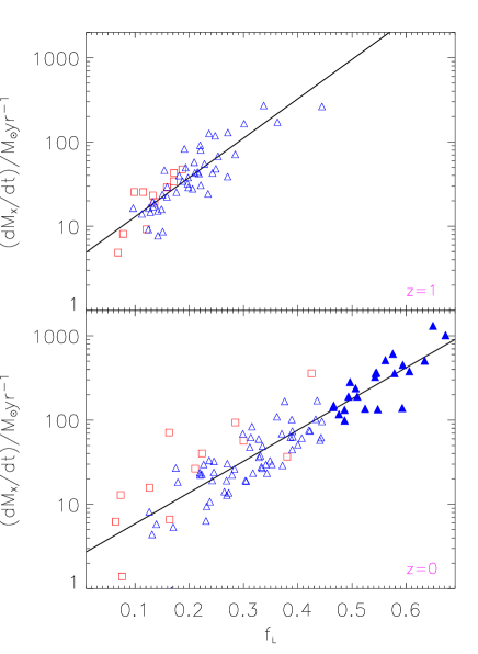
Figure 17: Inferred mass deposition rate from X-ray emission, $\dot{M}_{\rm X}$, versus X-ray concentration for regular (triangles) and irregular (squares) clusters at $z=1$ and $z=0$. Filled triangles are regular clusters with $f_{\rm L}>0.45$.

We have measured $\dot{M}_{\rm X}$ for our clusters (within a fixed physical radius of $r_{\rm core}=50\,h^{-1}\hbox{kpc}$) and, as expected, found that it is strongly correlated with $f_{\rm L}$, ranging from $\sim 1-900M_{\odot}{\rm yr}^{-1}$ (Fig. 17). Clusters with the highest concentrations, $f_{\rm L}>0.45$, are regular and typically have $\dot{M}_{\rm X}>100M_{\odot}{\rm yr}^{-1}$. These clusters could be called strong cooling-flow systems as they most resemble the observational samples of the same name; again note the absence of these objects at $z=1$.

While the median $f_{\rm L}$ decreases with redshift, the median $\dot{M}_{\rm X}$ stays approximately constant. The lack of strong cooling-flow clusters at high redshift is offset by the increase in $\dot{M}_{\rm X}$ for individual systems, due to the ratio, $r_{\rm core}/R_{500}$, being typically larger at higher redshift, thus capturing more of the cluster’s luminosity. Averaging over all redshifts, we found that $\left<\dot{M}_{\rm X}\right>=35\pm 5M_{\odot}{\rm yr}^{-1}$.

Here, we do not attempt to address the issue of how much gas is actually cooling down within our cluster cores. As discussed in K2004b, our simulations currently lack the number of particles to accurately follow the inward flow of the gas all the way down to low temperature. However, as we will demonstrate below, we find that the large range in X-ray concentration/cooling-flow strength exhibited by our clusters at low redshift is strongly dependent on the cluster’s larger-scale environment, i.e. whether it experienced a late-time major merger or not. So while the dynamics of a cooling core within a given cluster may not be accurate, and requires further investigation, our main (statistical) conclusions should hold as the simulation has accurately followed the merger histories of the cluster population.

5.2 Cooling flows, cool cores and dynamical state

Besides their high core luminosity, cooling-flow clusters have traditionally assumed to be dynamically-relaxed systems hosting a cool core. Conversely, non-cooling-flow clusters with low core luminosities are thought to host isothermal/warm cores and be dynamically disturbed. This view-point was recently challenged by McCarthy et al. (2004) as being overly-simplistic, as observations of both cooling-flow clusters with disturbed morphologies (e.g. Perseus) and non-cooling-flow clusters (e.g. 3C 129) with relaxed morphologies exist. Our simulation lends some support to their argument, as Fig. 17 shows. At $z=0$, irregular clusters are found to have a large range in $f_{\rm L}$ (or $\dot{M}_{\rm X}$), with one irregular cluster ($S_{\rm X}=0.14$) having $\dot{M}_{\rm X}=358M_{\odot}{\rm yr}^{-1}$. Conversely, regular clusters can also have very low X-ray concentrations ($\dot{M}_{\rm X}<10M_{\odot}{\rm yr}^{-1}$). However, statistically, the average regular cluster has a higher X-ray concentration than an irregular cluster. This is because the X-ray concentration is related to the dynamical history of the cluster, as we will show below.

We showed in subsection 3.5 that $f_{\rm L}$ is anti-correlated with the strength of the cool core, $f_{\rm T}$, as measured from the projected temperature profile; clusters with the coolest cores have more concentrated X-ray emission. However, nearly all of our clusters, regular and irregular, have cool cores ($f_{\rm T}<1$; Figs. 10 & 11). This is in agreement with previous simulation work where the gas was allowed to cool radiatively (e.g. Motl et al. 2004; Rowley, Thomas & Kay 2004; Poole et al. 2006), where it was found that cool cores are very hard to disrupt by mergers.

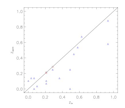
Figure 18: Redshift when each cluster last had a warm core versus the nearest redshift when it was irregular. Clusters that were regular (irregular) at $z_{\rm warm}$ are shown as triangles (squares). The solid line is $z_{\rm warm}=z_{\rm irr}$.

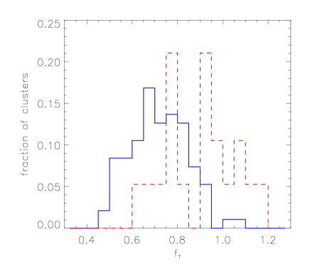
Figure 19: Distribution of $f_{\rm T}$ values at $z=0$ (solid histogram), compared to the observational sample of Sanderson, Ponman & O’Sullivan (2006).

Warm (or non-cool; $f_{\rm T}\geq 1$) cores exist but are rare in our simulation. Given the number of outputs available, only one quarter of the clusters were found to host a warm core since $z=1$, lasting at most around 1 Gyr. Interestingly, clusters with warm cores nearly always appear regular, even though the generation of a warm core appears linked to the merger process. This is shown in Fig. 18, where we see a clear correlation between the redshift when a cluster last had a warm core, $z_{\rm warm}$, against the nearest redshift when it was irregular ($S_{\rm X}>0.1$), $z_{\rm irr}$. It is unclear whether the cores are heated solely from the gravitational interaction of the merger, or a contribution comes from the feedback, which could also be triggered by a merger. Nevertheless, the paucity of warm cores is at odds with the observational data at low redshift. For example, Sanderson, Ponman & O’Sullivan (2006) recently studied a flux-limited sample of 20 clusters observed with Chandra, and found only half of them to contain cool cores, even though the core gas in the warm core clusters have cooling times significantly shorter than a Hubble time. The discrepancy is illustrated clearly in Fig. 19, where we compare the distribution of $f_{\rm T}$ values found in the CLEF simulation at $z=0$ with the observational data of Sanderson, Ponman & O’Sullivan (2006). Although based on a limited sample, the observations suggest there exists a bimodal distribution, not present in the simulation. This suggests that our simulation is still missing a heating mechanism that could produce a larger fraction of warm cores, which again could be linked to AGN activity.

5.3 Scatter in the L–T relation

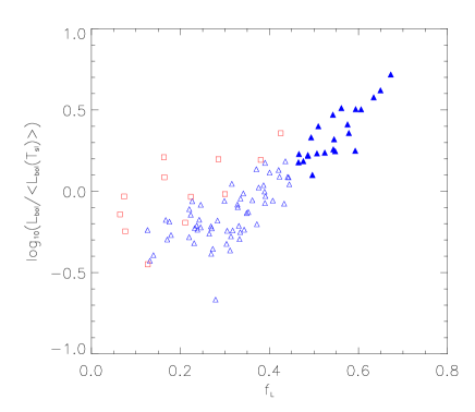
Figure 20: Offset in luminosity from the mean $L-T$ relation versus X-ray concentration for clusters at $z=0$. Triangles are regular clusters and squares irregular clusters. Solid triangles are clusters with the highest X-ray concentrations/X-ray-inferred mass deposition rates.

We now examine why there is a large scatter in the $L-T$ relation at low redshift. Classically, it is thought that the scatter is related to the dynamical histories of clusters. In particular, clusters with the strongest cooling flows (which lie above the mean $L-T$ relation) are believed to be in that state because they have not endured a major merger in the recent past. Our simulation supports this picture, as will be demonstrated in the following two figures. Firstly, Fig. 20 explicitly shows that the scatter in the $L-T$ relation is tightly correlated with the X-ray concentration (or mass deposition rate) of a cluster. For regular systems, clusters with higher X-ray concentrations lie above the mean relation, and those with low X-ray concentrations below. Irregular clusters lie off this correlation because $f_{\rm L}$ decreases due to the presence of a second object (which also boosts the luminosity).

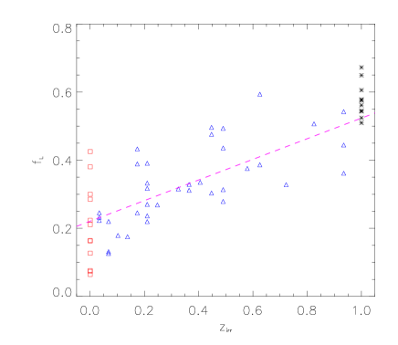
Figure 21: X-ray concentration at $z=0$ versus the lowest redshift when the cluster was irregular. Only clusters in our temperature-selected sample at all available redshifts, $z<z_{\rm irr}$, are plotted. Triangles are regular clusters today and squares irregular clusters ($z_{\rm irr}=0$). Asterisks are clusters with $z_{\rm irr}>1$, i.e. they did not experience a major merger between now and $z=1$. The dashed line is a best-fit relation to the regular clusters with $z_{\rm irr}<1$.

Secondly, in Fig. 21 we plot X-ray concentration at $z=0$ versus the lowest redshift when each cluster experienced a major merger. Clusters which are not present in our temperature-selected samples at all redshifts, $z<z_{\rm irr}$ are not plotted. Clearly there is a strongly-positive correlation, demonstrating that the most concentrated systems did not experience a major merger in the recent past (the asterisks are those clusters with $z_{\rm irr}>1$).

An alternative mechanism for generating the scatter was proposed by McCarthy et al. (2004), who used semi-analytic models of clusters with preheating and cooling (but the effects of accretion and merging of haloes were not included). They suggested that the position of a cluster on the luminosity–temperature relation was related to the level of preheating it received: clusters that experienced higher levels of preheating correspond to non-cooling-flow clusters (i.e. low X-ray concentrations, here) and vice-versa. Similarly to McCarthy et al. (2004), we tested whether the amount of feedback is correlated to the strength of the cooling core. Such an effect should be seen through a trend of stellar mass fraction with $f_{\rm L}$, as our feedback model injects energy approximately in proportion to the star-formation rate. No trend is seen in our simulation, i.e. stellar mass fractions are similar between clusters with low and high X-ray concentrations.

It is clear, therefore, that the strong cooling-flow population exists in our model at low redshift because of a lack of major merger activity in such systems at $z<1$. The absence of strong cooling-flow systems at higher redshift, responsible for the decrease in the $L-T$ scatter, can therefore be attributed to the increase in the merger rate with redshift.

The absence of strong cooling-flow clusters at high redshift in our model has important implications for cluster cosmology. Large samples of X-ray clusters at high redshift are still in their infancy, although will start to become available over the next few years, such as from the XMM-Newton Cluster Survey (Romer et al., 2001).

If our prediction is correct, it will have both positive and negative implications for cosmology. On the positive side, the smaller scatter will allow for a simpler survey selection function, with incompleteness effects being less of a problem. On the negative side, there is a lack of very luminous objects, so the number of high-redshift clusters above a given flux limit will be considerably less, reducing the overall power for specific surveys to constrain cosmological parameters. Interestingly, first observational results seem to support the lack of cooling-flow systems at high redshift (Vikhlinin et al., 2006b).

Another interesting point that our result throws up, is whether strong cooling-flow clusters would exist in a universe with $\Omega_{\rm m}=1$? In such a model, the merger rate would be expected to change very little with redshift, so clusters today may not have had the time to establish a strong cool core. In other words, the strongest cooling-flow clusters only exist because of the freeze-out of structure formation in a universe with sub-critical matter density.

6 Conclusions

In this paper, we presented the cluster population that forms within the CLEF simulation, an $N$-body/hydrodynamics simulation of the $\Lambda$CDM cosmology, with radiative cooling and energy feedback from galaxies. Our cluster sample, with nearly one hundred $kT>2$ keV objects at $z=0$ and sixty at $z=1$, is one of the largest drawn from a single simulation. In this paper, we studied the demographics of the cluster population out to $z=1$, focusing on the effects of dynamical activity and the strength of cooling cores, and how the X-ray properties of clusters depend on them. The Sunyaev–Zel’dovich properties of the clusters may be found in a companion paper (da Silva et al., in preparation). Our main conclusions are as follows:

• We quantified the amount of dynamical activity (major mergers) within the cluster population, using a simple projected substructure statistic, based on the observable X-ray surface-brightness distribution. While there is no significant dependence of this quantity, $S_{\rm X}$, with cluster temperature, it does increase with redshift. The fraction of irregular, $S_{\rm X}>0.1$ clusters, shown to be merging systems in the surface-brightness maps, increases from around 10 per cent at $z=0$ to 20 per cent at $z=1$, thus constituting a minority population at all redshifts.

• The projected ICM temperature profile of regular clusters has a generic shape at low and high redshift, decreasing in the centre (due to radiative cooling) and beyond $0.2R_{500}$, due to the intrinsic shape of the gravitational potential. Irregular clusters have flatter profiles at large radii due to the presence of a second object which compresses and heats the gas. The shape of the regular cluster profile at $z=0$ is in good agreement with the recent study of cool core clusters by Vikhlinin et al. (2005).

• To quantify the core properties of our clusters, we defined two simple (and observationally-measurable) structure parameters, $f_{\rm T}$, which measures the core to maximum temperature ratio, and $f_{\rm L}$ which measures the fraction of emission from within the core (the X-ray concentration of the cluster). We found that the vast majority of clusters contain cool cores ($f_{\rm T}<1$) at all redshifts. This is at odds with the observational data, at least at low redshift, where only half of clusters contain cool cores (Sanderson, Ponman & O’Sullivan, 2006). The X-ray concentration, $f_{\rm L}$, is anti-correlated with $f_{\rm T}$. The dispersion in $f_{\rm L}$ is large at $z=0$, but decreases with redshift due to the absence of clusters with the highest values (i.e. the strongest cooling cores).

• The scaled entropy profile has an outer logarithmic slope of 0.9 and decreases all the way into the centre, with no evidence of a flattened core. The ratio of the normalisation at large radii, for clusters at $z=1$ and $z=0$, is similar to that expected from the gravitational-heating model ($S(T)\propto E^{-4/3}(z)$), but the $z=1$ clusters have higher central entropy than at $z=0$. Irregular clusters have higher entropy profiles and regular clusters with strong cooling cores have lower entropy profiles. The profile at $z=0$ (in particular for the strong cooling core clusters) is in good agreement with the recent observational data of Pratt, Arnaud & Pointecouteau (2006).

• Mass estimates of X-ray clusters, based on the hydrostatic equilibrium equation, are around 20 per cent lower than the true masses, even when spatial density and temperature information of the ICM is known. As found by Rasia et al. (2006), the reasons for the discrepancy are X-ray temperature bias to low entropy gas and incomplete thermalisation of the gas.

• The estimated mass versus spectroscopic-like temperature relation at $z=0$ is only $\sim 10$ per cent higher than the observed relation for $R_{500}$. Splitting the regular cluster sample into those with weak and strong cooling cores makes little difference to the properties of the relation, when the temperature is measured outside the core. Thus, details of the mass–temperature relation should be insensitive to the cluster selection procedure.

• The mass–temperature relation evolves similarly to the gravitational-heating model prediction, $M(T)\propto E^{-1}(z)$. The scatter, $\Delta(\log M)\sim 0.08$, evolves very little with redshift.

• The luminosity–temperature relation has a large degree of scatter at $z=0$, reflecting the large dispersion in X-ray concentration of the clusters. Excising the core emission reduces the scatter considerably, although leads this to a relation that still has a higher normalisation than observed. Irregular clusters are not systematically offset from the main relation. The luminosity–temperature relation evolves negatively with redshift, contrary to the gravitational-heating expectation, where $L(T)\propto E(z)$. Excising the core reduces this negative evolution, with almost self-similar evolution at very low redshift.

• The scatter in the luminosity–temperature relation decreases strongly with redshift, again due to the lack of strong cooling core clusters at high redshift. There is a positive correlation between the X-ray concentration of the cluster and the redshift when it last had a major merger, but apparently not between the X-ray concentration and the level of feedback experienced by the cluster. Thus, our results indicate that the formation of a cooling-flow population of clusters at low redshift is tied to the slow down in dynamical activity in the $\Lambda$CDM model, allowing clusters in quieter environments to develop a strong cooling core.

Our simulation is one of the first of a new generation that is able to follow a substantial number of objects with reasonable resolution, while attempting to include the vital physical processes that alter the gravitationally-heated structure of the ICM: radiative cooling, star formation and feedback. While our particular model can reproduce many observed characteristic features of the cluster population, particularly those with cool cores, we acknowledge that it has its shortcomings. For example, it fails to completely quench the overcooling of baryons into stars, it does not predict enough clusters with warm cores, and it does not match the $L-T$ normalisation in detail (being too high).

All these problems point to the need for an even more efficient heating mechanism that reduces further the amount of cool gas in the clusters, without destroying the already good agreement in cool core clusters. It may be possible that the problems could be overcome by fine tuning the two feedback model parameters. However, it is desirable to incorporate a more realistic physical model for feedback, that is able to treat separately the effects from stars and black holes (in our current model, the heating rate directly follows the star-formation rate). The wealth of high-quality X-ray data that is becoming available will undoubtedly help constrain the feedback physics further, and thus allow more realistic cluster models to be constructed.

References

- Allen, Schmidt & Fabian (2001) Allen S.W., Schmidt R.W., Fabian A.C., 2001, MNRAS, 328, L37
- Arnaud & Evrard (1999) Arnaud M., Evrard A.E., 1999, MNRAS, 305, 631
- Arnaud, Pointecouteau & Pratt (2005) Arnaud M., Pointecouteau E., Pratt G.W., 2005, A&A, 441, 893
- Balogh et al. (2001) Balogh M.L., Pearce F.R., Bower R.G., Kay S.T., 2001, MNRAS, 326, 1228
- Balogh et al. (2006) Balogh M.L., Babul A., Voit G.M., McCarthy I.G., Jones L.R., Lewis G.F., Ebeling H., 2005, MNRAS, 366, 624
- Bauer et al. (2005) Bauer F.E., Fabian A.C., Sanders J.S., Allen S.W., Johnstone R.M., 2005, MNRAS, 359, 1481
- Bialek, Evrard & Mohr (2001) Bialek J.J., Evrard A.E., Mohr J.J., 2001, ApJ, 555, 597
- Blanchard & Bartlett (1998) Blanchard A., Bartlett J.G., 1998, A&A, 332, 49
- Borgani et al. (2002) Borgani S., Governato F., Wadsley J., Menci N., Tozzi P., Quinn T., Stadel J., Lake G., 2002, MNRAS, 336, 409
- Borgani et al. (2004) Borgani S., Murante G., Springel V., Diaferio A., Dolag K., Moscardini L., Tormen G., Tornatore L., Tozzi P., 2004, MNRAS, 348, 1078
- Bryan & Norman (1998) Bryan G.L., Norman, M., 1998, ApJ, 495, 80
- Buote & Tsai (1995) Buote D.A., Tsai J.C., 1995, ApJ, 452, 552
- Buote & Tsai (1996) Buote D.A., Tsai J.C., 1996, ApJ, 458, 27
- Crone, Evrard & Richstone (1996) Crone M.M., Evrard A.E., Richstone D.O., 1996, ApJ, 467, 489
- Davé, Katz & Weinberg (2002) Davé R., Katz N., Weinberg D.H., 2002, ApJ, 579, 23
- Davis et al. (1985) Davis M., Efstathiou G., Frenk C.S., White S.D.M., 1985, ApJ, 292, 371
- Edge & Stewart (1991) Edge A.C., Stewart G.C., 1991, MNRAS, 252, 414
- Eke, Navarro & Frenk (1998) Eke V.R., Navarro J.F., Frenk C.S., 1998, ApJ, 503, 569
- Eke et al. (1998) Eke V.R., Cole S.M., Frenk C.S., Henry J.P., 1998, MNRAS, 298, 1145
- Ettori et al. (2004) Ettori S., et al., 2004, MNRAS, 354, 111
- Ettori et al. (2006) Ettori S., Dolag K., Borgani S., Murante G., 2006, MNRAS, 365, 1021
- Evrard, Metzler & Navarro (1996) Evrard A.E., Metzler C.A., Navarro J.F., 1996, ApJ, 469, 494
- Fabian (2003) Fabian A.C., 2003, Cluster cores and cooling flows, Revista Mexicana de Astronomia y Astrofisica Conference Series, edited by V. Avila-Reese, C. Firmani and C. S. Frenk.
- Fabian et al. (1994) Fabian A.C., Crawford C.S., Edge A.C., Mushotzky R.F., 1994, MNRAS, 267, 779
- Finoguenov, Reiprich & Böhringer (2001) Finoguenov A., Reiprich T.H., Böhringer H., 2001, A&A, 368, 749
- Finoguenov, Böhringer & Zhang (2005) Finoguenov A., Böhringer H., Zhang Y.-Y., 2005, A&A, 442, 827
- Jeltema et al. (2005) Jeltema T.E., Canizares C.R., Bautz M.W., Buote D.A., 2005, ApJ, 624, 606
- Jones & Forman (1992) Jones C., Forman W., 1992, Clusters and Superclusters of Galaxies, Proceedings of NATO Advanced Study Institute, held at the Institute of Astronomy, July 1-10, 1991, Dordrecht: Kluwer, 1992, edited by A. C. Fabian. NATO Advanced Science Institutes (ASI) Series C, Volume 366, p.49
- Kaiser (1986) Kaiser N., 1986, MNRAS, 222, 323
- Kawahara et al. (2007) Kawahara H., Suto Y., Kitayama T., Sasaki S., Shimizu M., Rasia E., Dolag K., 2007, ApJ, in press (astro-ph/0611018)
- Kay, Thomas & Theuns (2003) Kay S.T., Thomas P.A., Theuns T., 2003, MNRAS, 343, 608
- Kay (2004) Kay S.T., 2004, MNRAS, 347, L13 (K2004a)
- Kay et al. (2004) Kay S.T., Thomas P.A., Jenkins A., Pearce F.R., 2004, MNRAS, 355, 1091 (K2004b)
- Kay et al. (2005) Kay S.T., et al. (the CLEF-SSH collaboration), 2005, Adv. Sp. Res., 36, 694 (Paper I)
- Kravtsov, Nagai & Vikhlinin (2005) Kravtsov A.V., Nagai D., Vikhlinin A.A., 2005, ApJ, 625, 588
- Lin, Mohr & Stanford (2003) Lin Y.-T., Mohr J.J., Stanford S.A., 2003, ApJ, 591, 749
- Markevitch (1998) Markevitch M., 1998, ApJ, 504, 27
- Mazzotta et al. (2004) Mazzotta P., Rasia E., Moscardini L., Tormen G., 2004, MNRAS, 354, 10
- McCarthy et al. (2004) McCarthy I.G., Balogh M.L., Babul A., Poole G.B., Horner D.J., 2004, ApJ, 613, 811
- Mohr, Fabricant & Geller (1993) Mohr J.J., Fabricant D.G., Geller M.J., 1993, ApJ, 413, 492
- Motl et al. (2004) Motl P.M., Burns J.O., Loken C., Norman M.L., Bryan G., 2004, ApJ, 606, 635
- Muanwong et al. (2001) Muanwong O., Thomas P.A., Kay S.T., Pearce F.R., Couchman H.M.P., 2001, ApJ, 552, L27
- Muanwong et al. (2002) Muanwong O., Thomas P.A., Kay S.T., Pearce F.R., 2002, MNRAS, 336, 527
- Muanwong, Kay & Thomas (2006) Muanwong O., Kay S.T., Thomas P.A., 2006, ApJ, 649, 640
- Navarro, Frenk & White (1995) Navarro J.F., Frenk C.S., White S.D.M., 1995, MNRAS, 275, 720
- O’Hara et al. (2006) O’Hara T.B., Mohr J.J., Bialek J.J., Evrard A.E., 2006, ApJ, 639, 640
- Onuora, Kay & Thomas (2003) Onuora L.I., Kay S.T., Thomas P.A., 2003, MNRAS, 341, 1246
- Pearce et al. (2000) Pearce F.R., Thomas P.A., Couchman H.M.P., Edge A.C., 2000, MNRAS, 317, 1029
- Piffaretti et al. (2005) Piffaretti R., Jetzer Ph., Kaastra J.S., Tamura T., 2005, A&A, 433, 101
- Ponman, Cannon & Navarro (1999) Ponman T.J., Cannon D.B., Navarro J.F., 1999, Nature, 397, 135
- Ponman, Sanderson & Finoguenov (2003) Ponman T.J., Sanderson A.J.R., Finoguenov A., 2003, MNRAS, 343, 331
- Poole et al. (2006) Poole G.B., Fardal M.A., Babul A., McCarthy I.G., Quinn T., Wadsley J., 2006, MNRAS, accepted (astro-ph/0608560)
- Pratt & Arnaud (2003) Pratt G.W., Arnaud M., 2003, A&A, 408,1
- Pratt, Arnaud & Pointecouteau (2006) Pratt G.W., Arnaud M., Pointecouteau E., 2006, A&A, 446, 429
- Pratt et al (2007) Pratt G.W., Böhringer H., Croston J.H., Arnaud M., Borgani S., Finoguenov A., Temple R.F., 2007, A&A, 461, 71
- Rasia et al. (2004) Rasia E., Tormen G., Moscardini L., 2004, MNRAS, 351, 237
- Rasia et al. (2005) Rasia E., Mazzotta P., Borgani S., Moscardini L., Dolag K., Tormen G., Diaferio A., Murante G., 2005, ApJ, 618, L1
- Rasia et al. (2006) Rasia E., Ettori S., Moscardini L., Mazzotta P., Borgani S., Dolag K., Tormen G., Cheng L.M., Diaferio A., 2006, MNRAS, 369, 201
- Romer et al. (2001) Romer A.K., Viana P.T.P., Liddle A.R., Mann R.G., 2001, ApJ, 547, 594
- Rowley, Thomas & Kay (2004) Rowley D.R., Thomas P.A., Kay S.T., 2004, MNRAS, 352, 508
- Sanderson, Ponman & O’Sullivan (2006) Sanderson A.J.R., Ponman T.J., O’Sullivan E., 2006, MNRAS, accepted (astro-ph/0608423)
- Schuecker et al. (2001) Schuecker P., Böhringer H., Reiprich T.H., Feretti L., 2001, A&A, 378, 408
- Seljak & Zaldarriaga (1996) Seljak U., Zaldarriaga M., 1996, ApJ, 469, 437
- Spergel et al. (2003) Spergel D.N. et al., 2003, ApJS, 148, 175
- Springel & Hernquist (2002) Springel V., Hernquist L., 2002, MNRAS, 333, 649
- Springel (2006) Springel V., 2006, MNRAS, 364, 1105
- Sutherland & Dopita (1993) Sutherland R., Dopita M.S., 1993, ApJS, 88, 253
- Thomas & Couchman (1992) Thomas P.A., Couchman H.M.P., 1992, MNRAS, 257, 11
- Thomas et al. (1998) Thomas P.A. et al., 1998, MNRAS, 296, 1061
- Tornatore et al. (2003) Tornatore L., Borgani S., Springel V., Matteucci F., Menci N., Murante G., 2003, MNRAS, 342,1025
- Tozzi et al. (2003) Tozzi P., Rosati P., Ettori S., Borgani S., Mainieri V., Norman C., 2003, ApJ, 593, 705
- Tozzi & Norman (2001) Tozzi P., Norman C., 2001, ApJ, 546, 63
- Valdarnini (2003) Valdarnini R., 2003, MNRAS, 339, 111
- Vikhlinin et al. (2005) Vikhlinin A., Markevitch M., Murray S. S., Jones C., Forman W., Van Speybroeck L., 2005, ApJ, 628, 655
- Vikhlinin et al. (2006a) Vikhlinin A., Kravtsov A., Forman W., Jones C., Markevitch M., Murray S. S., Van Speybroeck L., 2006a, ApJ, 640, 691
- Vikhlinin et al. (2006b) Vikhlinin A., Burenin R., Forman W.R., Jones C., Hornstrup A., Murray S.S., Quintana H., 2006b, to appear in proceedings of “Heating vs. Cooling in Galaxies and Clusters of Galaxies” (astro-ph/0611438)
- Voit (2005) Voit G.M., 2005, Rev. Mod. Phys., 77, 207
- Voit, Kay & Bryan (2005) Voit G.M., Kay S.T., Bryan G.L., 2005, MNRAS, 364, 909
- Zhang et al. (2006) Zhang Y.-Y., Böhringer H., Finoguenov A., Ikebe Y., Matsushita K., Schuecker P., Guzzo L., Collins C.A., 2006, A&A, 456, 55