Tracing the evolution in the iron content of the ICM

We present a Chandra analysis of the X-ray spectra of 56 clusters of galaxies at $z>0.3$, which cover a temperature range of $3>kT>15$ keV. Our analysis is aimed at measuring the iron abundance in the ICM out to the highest redshift probed to date. We find that the emission-weighted iron abundance measured within $(0.15-0.3)\,R_{vir}$ in clusters below 5 keV is, on average, a factor of $\sim 2$ higher than in hotter clusters, following $Z(T)\simeq 0.88\,T^{-0.47}\,Z_{\odot}$, which confirms the trend seen in local samples. We made use of combined spectral analysis performed over five redshift bins at $0.3>z>1.3$ to estimate the average emission weighted iron abundance. We find a constant average iron abundance $Z_{Fe}\simeq 0.25\,Z_{\odot}$ as a function of redshift, but only for clusters at $z>0.5$. The emission-weighted iron abundance is significantly higher ($Z_{Fe}\simeq 0.4\,Z_{\odot}$) in the redshift range $z\simeq 0.3-0.5$, approaching the value measured locally in the inner $0.15\,R_{vir}$ radii for a mix of cool-core and non cool-core clusters in the redshift range $0.1<z<0.3$. The decrease in $Z_{Fe}$ with $z$ can be parametrized by a power law of the form $\sim(1+z)^{-1.25}$. The observed evolution implies that the average iron content of the ICM at the present epoch is a factor of $\sim 2$ larger than at $z\simeq 1.2$. We confirm that the ICM is already significantly enriched ($Z_{Fe}\simeq 0.25\,Z_{\odot}$) at a look-back time of 9 Gyr. Our data provide significant constraints on the time scales and physical processes that drive the chemical enrichment of the ICM.

1 Properties of the sample and spectral analysis

The selected sample consists of all the public Chandra archived observations of clusters with $z\geq 0.4$ as of June 2004, including 9 clusters with $0.3<z<0.4$. We used the XMM-Newton data to boost the S/N only for the most distant clusters in our current sample, namely the clusters at $z>1$.

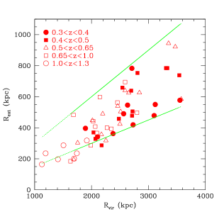
We performed a spectral analysis extracting the spectrum of each source from a region defined in order to maximize the S/N ratio. As shown in Fig. 1, in most cases the extraction radius $R_{ext}$ is between 0.15 and 0.3 virial radius $R_{vir}$. The spectra were analyzed with XSPEC v11.3.1 arn96 and fitted with a single-temperature mekal model kaa92 ; lie95 in which the ratio between the elements was fixed to the solar value as in and89 .

Figure 1: Left: extraction radius $R_{ext}$ versus $R_{vir}$. Lower and upper lines show $R_{ext}=0.15\,R_{vir}$ and $R_{ext}=0.3\,R_{vir}$, respectively. Right: temperature vs redshift. Shaded areas show the rms dispersion around the weighted mean in different redshift bins.

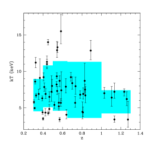
We show in Fig. 1 the distribution of temperatures in our sample as a function of redshifts (error bars are at the $1\sigma$ c.l.). The Spearman test shows no correlation between temperature and redshift ($r_{s}=-0.095$ for 54 d.o.f., probability of null correlation $p=0.48$). Fig. 1 shows that the range of temperatures in each redshift bin is about $6-7$ keV. Therefore, we are sampling a population of medium-hot clusters uniformly with $z$, with the hottest clusters preferentially in the range $0.4<z<0.6$.

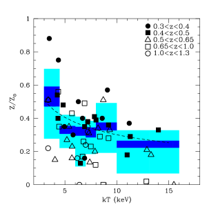
Our analysis suggests higher iron abundances at lower temperatures in all the redshift bins. This trend is somewhat blurred by the large scatter. We find a more than $2\sigma$ negative correlation for the whole sample, with $r_{s}=-0.31$ for 54 d.o.f. ($p=0.018$). The correlation is more evident when we compute the weighted average of $Z_{Fe}$ in six temperature intervals, as shown by the shaded areas in Fig. 2.

Figure 2: Left: scatter plot of best-fit $Z_{Fe}$ values versus $kT$. The dashed line represents the best-fit $Z-T$ relation ($Z/Z_{\odot}\simeq 0.88\,T^{-0.47}$). Shaded areas show the weighted mean (blue) and average $Z_{Fe}$ with rms dispersion (cyan) in 6 temperature bins. Right: mean $Z_{Fe}$ from combined fits (red circles) and weighted average of single-source measurements (black squares) within 6 redshift bins. The triangles at $z\simeq 0.2$ are based on the low-z sample described in Sect. 2. Error bars refer to the $1\sigma$ c.l.. Shaded areas show the rms dispersion. The dashed line indicates the best fit over the 6 redshift bins for a simple power law of the form $\langle Z_{Fe}\rangle=Z_{Fe}(0)\,(1+z)^{-1.25}$.

2 The evolution of the iron abundance with redshift

The single-cluster best-fit values of $Z_{Fe}$ decrease with redshift. We find a $\sim 3\sigma$ negative correlation between $Z_{Fe}$ and $z$, with $r_{s}=-0.40$ for 54 d.o.f. ($p=0.0023$). The decrease in $Z_{Fe}$ with $z$ becomes more evident by computing the average iron abundance as determined by a combined spectral fit in a given redshift bin. This technique is similar to the stacking analysis often performed in optical spectroscopy, where spectra from a homogeneous class of sources are averaged together to boost the S/N, thus allowing the study of otherwise undetected features. In our case, different X-ray spectra cannot be stacked due to their different shape (different temperatures). Therefore, we performed a simultaneous spectral fit leaving temperatures and normalizations free to vary, but using a unique metallicity for the clusters in a narrow $z$ range.

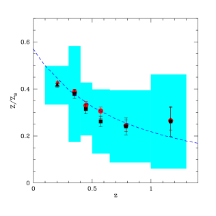
The $Z_{Fe}$ measured from the combined fits in 6 redshift bins is shown in Fig. 2. We also computed the weighted average from the single cluster fits in the same redshift bins. The best-fit values resulting from the combined fits are always consistent with the weighted means within $1\sigma$ (see Fig. 2). This allows us to measure the evolution of the average $Z_{Fe}$ as a function of redshift, which can be modelled with a power law of the form $\sim(1+z)^{-1.25}$.

Since the extrapolation of the average $Z_{Fe}$ at low-$z$ points towards $Z_{Fe}(0)\simeq 0.5\,Z_{\odot}$, we need to explain the apparent discrepancy with the oft-quoted canonical value $\langle Z_{Fe}\rangle\simeq 0.3\,Z_{\odot}$. The discrepancy is due to the fact that our average values are computed within $r\simeq 0.15\,R_{vir}$, where the iron abundance is boosted by the presence of metallicity peaks often associated to cool cores. The regions chosen for our spectral analysis, are larger than the typical size of the cool cores, but smaller than the typical regions adopted in studies of local samples. In order to take into account aperture effects, we selected a small subsample of 9 clusters at redshift $0.1<z<0.3$, including 7 cool-core and 2 non cool-core clusters, a mix that is representative of the low-$z$ population. These clusters are presently being analyzed for a separate project aimed at obtaining spatially-resolved spectroscopy (Baldi et al., in preparation). Here we analyze a region within $r=0.15\,R_{vir}$ in order to probe the same regions probed at high redshift. We used this small control sample to add a low-$z$ point in our Fig. 2, which extends the $Z_{Fe}$ evolutionary trend.

3 Discussion

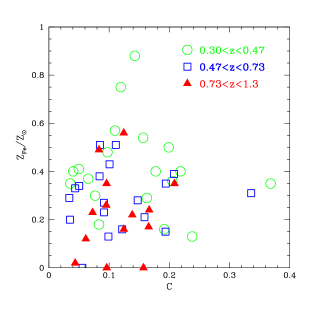
We investigate whether the evolution of $Z_{Fe}$ could be due to an evolving fraction of clusters with cool cores, which are known to be associated with iron-rich cores deg04 and which amount to more than 2/3 of the local clusters bau05 . In order to use a simple characterization of cool-core clusters in our high-z sample, we computed the ratio of the fluxes emitted within 50 and 500 kpc ($C=f(r<50\,kpc)/f(r<500\,kpc$) computed as the integral of the surface brightness in the $0.5-5$ keV band (observer frame). This quantity ranges between 0 and 1 and it represents the relative weight of the central surface brightness. Higher values of $C$ are expected if a cool core is present. If the decrease in $Z_{Fe}$ with redshift is associated to a decrease in the number of cool-core clusters for higher $z$, we would expect to observe a positive correlation between $Z_{Fe}$ and $C$ and a negative correlation between $C$ and $z$. In Fig. 3 we plot $Z_{Fe}$ as a function of $C$ for our sample. We find that in our sample there is no correlation between metallicity and $C$ with a Spearman’s coefficient of $r_{s}=0.02$ (significance of $\sim 0.2\sigma$) nor one between $C$ and $z$ ($r_{s}=-0.11$, a level of confidence of $0.8\sigma$).

The absence of strong correlations between $C$ and $Z_{Fe}$ or between $C$ and $z$ suggests that the mix of cool cores and non cool cores over the redshift range studied in the present work cannot justify the observed evolution in the iron abundance. We caution, however, that a possible evolution of the occurrence of cool-core clusters at high redshift may still partially contribute to the observed evolution of $Z_{Fe}$. In other words, whether the observed evolution of $Z_{Fe}$ is contributed entirely by the evolution of the mass of iron or is partially due to a redistribution of iron in the central regions of clusters is an open issue to be addressed with a proper and careful investigation of the surface brightness of the high-z sample.

Figure 3: Left: iron abundance plotted versus $C=f(r<50\,kpc)/f(r<500\,kpc)$. Clusters within different redshift bins are coded with different symbols. Right: iron abundance plotted versus the ratio $R_{ext}/R_{vir}$. Shaded areas show the rms dispersion around the average iron abundance in four bins.

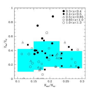
A final check is provided by the scatter plot of $Z_{Fe}$ versus $R_{ext}/R_{vir}$, shown in Fig. 3. We do not detect any dependence of $Z_{Fe}$ on the extraction radius adopted for the spectral analysis. In particular, we find that clusters with smaller extraction radii do not show higher $Z_{Fe}$ values.

4 Conclusions

We have presented the spectral analysis of 56 clusters of galaxies at intermediate-to-high redshifts observed by Chandra and XMM-Newton bal06 . This work improves our first analysis aimed at tracing the evolution of the iron content of the ICM out to $z>1$ toz03 , by substantially extending the sample. The main results of our work can be summarized as follows:

• We determine the average ICM iron abundance with a $\sim 20$% uncertainty at $z>1$ ($Z_{Fe}=0.27\pm 0.05\,Z_{\odot}$), thus confirming the presence of a significant amount of iron in high-$z$ clusters. $Z_{Fe}$ is constant above $z\simeq 0.5$, the largest variations being measured at lower redshifts.

• We find a significantly higher average iron abundance in clusters with $kT<5$ keV, in agreement with trends measured in local samples. For $kT>3$ keV, $Z_{Fe}$ scales with temperature as $Z_{Fe}(T)\simeq 0.88\,T^{-0.47}$.

• We find significant evidence of a decrease in $Z_{Fe}$ as a function of redshift, which can be parametrized by a power law $\langle Z_{Fe}\rangle\simeq Z_{Fe}(0)\,(1+z)^{-\alpha_{z}}$, with $Z_{Fe}(0)\simeq 0.54\pm 0.04$ and $\alpha_{z}\simeq 1.25\pm 0.15$. This implies an evolution of more than a factor of 2 from $z=0.4$ to $z=1.3$.

We carefully checked that the extrapolation towards $z\simeq 0.2$ of the measured trend, pointing to $Z_{Fe}\simeq 0.5\,Z_{\odot}$, is consistent with the values measured within a radius $r=0.15\,R_{vir}$ in local samples including a mix of cool-core and non cool-core clusters. We also investigated whether the observed evolution is driven by a negative evolution in the occurrence of cool-core clusters with strong metallicity gradients towards the center, but we do not find any clear evidence of this effect. We note, however, that a proper investigation of the thermal and chemical properties of the central regions of high-z clusters is necessary to confirm whether the observed evolution by a factor of $\sim 2$ between $z=0.4$ and $z=1.3$ is due entirely to physical processes associated with the production and release of iron into the ICM, or partially associated with a redistribution of metals connected to the evolution of cool cores.

Precise measurements of the metal content of clusters over large look-back times provide a useful fossil record for the past star formation history of cluster baryons. A significant iron abundance in the ICM up to $z\simeq 1.2$ is consistent with a peak in star formation for proto-cluster regions occurring at redshift $z\simeq 4-5$. On the other hand, a positive evolution of $Z_{Fe}$ with cosmic time in the last 5 Gyrs is expected on the basis of the observed cosmic star formation rate for a set of chemical enrichment models. Present constraints on the rates of SNae type Ia and core-collapse provide a total metal produciton in a typical X-ray galaxy cluster that well reproduce (i) the overall iron mass, (ii) the observed local abundance ratios, and (iii) the measured negative evolution in $Z_{Fe}$ up to $z\simeq 1.2$ ett06 .

References

- (1) Anders, E. & Grevesse, N. 1989, Geochim. Cosmochim. Acta, 53, 197
- (2) Arnaud, K. A. 1996, in ASP Conf. Ser. 101: Astronomical Data Analysis Software and Systems V, ed. G. H. Jacoby & J. Barnes, 17–+
- (3) Balestra, I., Tozzi, P., Ettori, S., et al. 2006, A&A, in press (astro-ph/0609664)
- (4) Bauer, F. E., Fabian, A. C., Sanders, J. S., et al. 2005, MNRAS, 359, 1481
- (5) De Grandi, S., Ettori, S., Longhetti, M., & Molendi, S. 2004, A&A, 419, 7
- (6) Ettori, S. 2006, in these proceedings (astro-ph/0610466)
- (7) Kaastra, J. S. 1992, (Internal SRON–Leiden Report, updated version 2.0)
- (8) Liedahl, D. A., Osterheld, A. L., & Goldstein, W. H. 1995, ApJl, 438, L115
- (9) Tozzi, P., Rosati, P., Ettori, S., et al. 2003, ApJ, 593, 705