The synthesis of the cosmic X-ray background
in the Chandra and XMM-Newton era

We present a detailed and self-consistent modeling of the cosmic X-ray background (XRB) based on the most up-to-date X-ray luminosity functions (XLF) and evolution of Active Galactic Nuclei (AGN). The large body of observational results collected by soft (0.5-2 keV) and hard (2-10 keV) X-ray surveys are used to constrain at best the properties of the Compton-thin AGN population and its contribution to the XRB emission. The number ratio $R$ between moderately obscured (Compton-thin) AGN and unobscured AGN is fixed by the comparison between the soft and hard XLFs, which suggests that $R$ decreases from 4 at low luminosities to 1 at high luminosities. From the same comparison there is no clear evidence of an evolution of the obscured AGN fraction with redshift. The distribution of the absorbing column densities in obscured AGN is determined by matching the soft and hard source counts. A distribution rising towards larger column densities is able to reproduce the soft and hard AGN counts over about 6 dex in flux. The model also reproduces with excellent accuracy the fraction of obscured objects in AGN samples selected at different X-ray fluxes. The integrated emission of the Compton-thin AGN population is found to underestimate the XRB flux at about 30 keV, calling for an additional population of extremely obscured (Compton-thick) AGN. Since the number of Compton-thick sources required to fit the 30 keV XRB emission strongly depends on the spectral templates assumed for unobscured and moderately obscured AGN, we explored the effects of varying the spectral templates. In particular, in addition to the column density distribution, we also considered a distribution in the intrinsic powerlaw spectral indices of variable width. In our baseline model a Gaussian distribution of photon indices with mean $\langle\Gamma\rangle=1.9$ and dispersion $\sigma_{\Gamma}=0.2$ is assumed. This increases the contribution of the Compton-thin AGN population to the 30 keV XRB intensity by $\sim 30\%$ with respect to the case of null dispersion (i.e. a single primary AGN powerlaw with $\Gamma=1.9$) but is not sufficient to match the 30 keV XRB emission. Therefore a population of heavily obscured -Compton-thick- AGN, as large as that of moderately obscured AGN, is required to fit the residual background emission. Remarkably, the fractions of Compton-thick AGN observed in the Chandra Deep Field South and in the first INTEGRAL and Swift catalogs of AGN selected above 10 keV are in excellent agreement with the model predictions.

1 Introduction

After more than 40 years since its discovery (Giacconi et al. 1962), it is by now clear that the cosmic X-ray background (XRB) is produced by the integrated emission of faint extragalactic point–like sources. In the deepest X-ray surveys to date, i.e. the 800 ksec XMM-Newton Lockman Hole (Hasinger 2004), the 1 Msec Chandra Deep Field South (CDFS, Giacconi et al. 2002) and the 2 Msec Chandra Deep Field North (CDFN, Alexander et al. 2003), the summed X-ray fluxes of the detected sources account for virtually the entire XRB emission around a few keV and for about half of that at higher (7–10 keV) energies (Worsley et al. 2005), the exact fraction depending on the absolute XRB flux which is still affected by rather large uncertainties. The measurements performed by the HEAO1–A2 experiment (Marshall et al. 1980), which provided the only broad band (3–100 keV) XRB spectrum available to date, has the lowest normalization. More recent values, obtained below 10 keV with imaging instruments, were found to be always higher, the highest one having been measured by BeppoSAX (Vecchi et al. 1999). The most recent determinations of the XRB flux by RXTE (Revnivtsev et al. 2003), XMM-Newton (Lumb et al. 2002; De Luca & Molendi 2004) and Chandra (Hickox & Markevitch 2006) as well as a reanalysis of the HEAO1–A2 data (Revnivtsev et al. 2005) have been found to lay in between the original HEAO1–A2 measure and the BeppoSAX one, comparable to those obtained a few years ago by ASCA (Gendreau et al. 1995; Kushino et al. 2002). It is worth mentioning that, on the basis of a careful determination of the unresolved X–ray background in Chandra deep fields, Hickox & Markevitch (2006) concluded that the contribution of resolved sources accounts for $\sim 80\%$ of the 0.5–8 keV Chandra flux which, in the 2–8 keV band, corresponds to the entire HEAO1–A2 flux. At energies $>$ 10 keV, where the bulk of the XRB energy resides, the only available measure is that of HEAO1. Whether the high energy flux should be renormalized upwards by $\sim 30\%$ (see e.g. Ueda et al. 2003) or the very shape of the broad band spectrum is different from that originally observed is still the subject of debate (see Gilli 2004 and Revnivtsev et al. 2005 for recent discussions). The issue of the XRB intensity, especially around its 30 keV peak, bears important consequences for the energy released through accretion onto supermassive black holes integrated over the cosmic history. Indeed, extensive optical follow–up programs have shown that the vast majority of the XRB sources are identified as Active Galactic Nuclei (AGN) with different degrees of obscuration (e.g. Szokoly et al. 2004, Barger et al. 2005) confirming early predictions by AGN synthesis models (Setti & Woltjer 1989, Comastri et al. 1995). Among the many issues which are currently subject of intense research activity there are: a complete census of the entire AGN population and especially of the most obscured objects; the space density of obscured sources as a function of redshift and intrinsic X–ray luminosity; the demography of high redshift ($z>$ 3) quasars; the black hole mass function; the average radiative efficiency and Eddington ratios of accreting supermassive black holes.

In order to properly address the above described scientific goals, the most efficient approach is to combine deep pencil beam Chandra and XMM–Newton pointings with shallower surveys over much larger sky areas (e.g. the ASCA Medium and Large Sensitivity Surveys; Ueda et al. 2001; the HELLAS and HELLAS2XMM surveys; Fiore et al. 2001, 2003). The extensive multiwavelength coverage available, though at different levels of sensitivity for the various X–ray surveys, allows to sample the X–ray sky source content over several orders of magnitude in the X–ray flux and has already provided statistically meaningful (several hundreds) samples of AGN across a wide range of redshifts, luminosities and obscuring column densities.

The redshift distribution of AGN selected both in the soft (0.5–2 keV) and hard (2–10 keV) X–ray band peaks at $z\simeq$ 0.7–1.0 and is dominated by low luminosity objects (log L_X=42–44 erg s^-1). The observed distribution is in contrast with the predictions by simple models based on pure luminosity evolution (PLE) or pure density evolution (PDE) of AGN through cosmic times, and has led to a more complicated scenario. Indeed, the evolution of the X–ray selected AGN luminosity function up to redshifts of $\sim$ 3–4 is described, both in the soft (Hasinger, Miyaji & Schmidt 2005) and hard (Ueda et al. 2003, La Franca et al. 2005, Barger et al. 2005) X–ray bands, by a luminosity dependent density evolution model (LDDE) whose best fit parameters imply a strong dependence of the AGN space density and evolution with X–ray luminosity. More specifically, a clear trend for an increase of the peak redshift for increasing X–ray luminosity of the AGN space density is present. The comoving space density of luminous (log $L_{X}>44$) quasars peaks at $z\simeq$ 2–2.5 and declines rapidly, by more than two orders of magnitude, towards $z=0$, in marked contrast with the behavior of lower luminosity AGN, whose space density increases by less than a factor 10 from $z=0$ to $z\simeq$ 0.7–1 and decreases thereafter.

Given that luminous quasars are on average expected to be powered by more massive black holes than lower luminosity AGN, the luminosity dependent evolution of AGN space density bears some similarities with the evolution of the star formation history and mass assembly of non-active galaxies and is often considered as a strong evidence of the co-evolution of supermassive black holes and their host galaxies. The cosmic downsizing of the AGN population can be explained assuming that rare, massive black holes powering high redshift luminous quasars are quickly formed and efficiently fed at early cosmic times in a gas and dust rich environment, which makes possible accretion at high Eddington ratios. The bulk of lower luminosity AGN population has to wait much longer to grow and/or to be activated, possibly due to the lack of large reservoir of gas which limits the accretion to a sub-Eddington regime (see e.g Hopkins et al. 2006 and references therein).

According to the above described theoretical framework a large population of obscured high redshift quasars is predicted. While it has been proposed that they could be associated with high-redshift submm sources (Alexander et al. 2005), the actual size of the obscured QSO population at high redshift is however still largely debated. The most recent results from the largest compilations of X-ray surveys and X-ray background synthesis models provide contradictory results, sometimes favoring an increase of the obscured AGN fraction with redshift (e.g. La Franca et al. 2005, Ballantyne et al. 2006), sometimes favoring a constant fraction (Ueda et al. 2003, Treister & Urry 2005). On the contrary, evidence for a dependence of the fraction of obscured AGN on the intrinsic source luminosity is rapidly growing, the fraction of obscured QSOs being significantly lower than the corresponding fraction of obscured Seyferts (Ueda et al. 2003, Hasinger 2004, La Franca et al. 2005, Georgakakis et al. 2006).

Another still open and challenging issue, strictly related with that of obscured high redshift quasars, concerns the number density of heavily obscured, Compton-thick sources. Although X–ray observations are the least biased against obscured AGN, nonetheless sensitive imaging surveys can be performed at present only at energies below 10 keV and are therefore expected to severely undersample the number of extremely obscured AGN with column densities above log$N_{H}=24$ (i.e. Compton-thick sources). In the local Universe Compton-thick AGN are found to be as numerous as moderately obscured AGN (Risaliti et al. 1999; Guainazzi et al. 2005) and are expected to provide a significant contribution to the 30 keV peak in the XRB spectrum (Comastri et al. 1995; Gilli et al. 2001). A full, self-consistent modeling of the XRB spectrum which takes into account all the available observational constraints appears to be, at present, the most effective way to characterize the population of heavily obscured Compton–thick AGN and thus to have a complete map of the AGN demography. The space density and redshift distribution of Compton-thick AGN is particularly relevant to properly estimate the supermassive black hole mass function and, by comparison with the relic black hole mass distribution of local galaxies, to constrain the average Eddington ratio and radiative efficiency averaged over the cosmic times (Marconi et al. 2004).

Throughout this paper a flat cosmological model with $\Omega_{m}=1-\Omega_{\Lambda}=0.3$, $H_{0}=70\,h_{70}$ km s^-1 Mpc^-1 is assumed.

2 Model outline

The wealth of X–ray data collected by sensitive imaging surveys in the 0.5–10 keV energy range, complemented by optical and near infrared photometric and spectroscopic identification programs which have reached a high degree of completeness, allows us to tightly constrain the contribution of unobscured and Compton-thin AGN to the XRB. Once the overall properties of these AGN are constrained at best of our present knowledge (e.g. source counts, luminosity functions and redshift distributions, resolved XRB fraction) it is possible to compute their contribution to the 0.5–300 keV XRB emission, for reasonable assumptions on their spectral shape above 10 keV, and then estimate the abundance of Compton-thick AGN by adding as many sources as required to fit the residual (i.e. not accounted for by unobscured and Compton-thin AGN) XRB intensity.

Given the well known discrepancies among different XRB measurements, which still have to be fully understood, we will not adopt the XRB emission below 10 keV as a primary model constraint. Rather, we rely on what we believe to be more robust observational data such as the 0.5-2 keV and 2-10 keV logN–logS and luminosity functions and verify a posteriori the resulting XRB spectrum. As far as the absolute intensity of the 30 keV peak is concerned we will adopt the only available HEAO1–A2 measurement (Marshall et al. 1980) as a reference value. We discuss in Section 9.3 the implications of a higher level of the $>$ 10 keV XRB

More specifically the adopted strategy is as follows:

The 0.5–2 keV type-1 AGN luminosity function recently computed by Hasinger, Miyaji & Schmidt (2005) is assumed as the XLF of X–ray unobscured AGN (log$N_{H}<21$), while the 2–10 keV AGN luminosity functions obtained by Ueda et al. (2003) and La Franca et al. (2005) are assumed to represent the total XLF of unobscured plus Compton-thin (log$N_{H}<24$) AGN.

The soft XLF of unobscured AGN is converted in the 2–10 keV band assuming a distribution for the X–ray spectral slopes of unobscured AGN. The average value and dispersion are chosen to match those observed for relatively bright X–ray selected type-1 AGN.

The difference between the observed 2–10 keV XLF and the one determined for unobscured AGN provides the total number of obscured Compton-thin AGN ($21<$log$N_{H}<24$). The comparison between the XLFs is also used to verify if there are variations in the ratio between obscured and unobscured AGN as a function of redshift and/or luminosity.

Once the total number of obscured Compton-thin AGN is determined, their absorption distribution is found by fitting the source counts in the 0.5–2 keV, 2–10 keV and 5–10 keV bands. When the absorption distribution is determined, the population of unobscured and Compton-thin AGN is fully characterized.

Assuming an accurate modeling of the X–ray spectra of Compton-thin AGN over the 0.5 - 400 keV energy range, including X–ray absorption, a reflection component and a high energy exponential cut–off, their contribution to the broad band XRB spectrum is computed.

The number of Compton-thick sources is then determined by adding as many sources as needed to fit the residual XRB intensity, in particular the XRB peak at 30 keV.

At this stage the model is checked for self-consistency by recomputing the source counts in the various bands and the fraction of obscured AGN as a function of the X–ray flux, taking into account the contribution of Compton-thick AGN. Finally, we compute the model predictions beyond the present observational limits and in particular the expected fraction of Compton-thick AGN as a function of the survey depth and energy range (i.e. below and above about 10 keV).

3 AGN X-ray spectra

3.1 Unobscured AGN

The average X–ray spectral properties of AGN are relatively well known over a broad range of luminosities and redshifts. The main spectral component is a power law with an exponential roll over at high (above 100 keV) energies. The average slope of the power law component as measured for large samples of low-luminosity Seyfert galaxies (i.e. Nandra & Pounds 1994) and bright QSOs (Reeves & Turner 2000, Piconcelli et al. 2005) is close to $\Gamma$=1.9 without any significant redshift dependence up to $z\lesssim 5$ (Vignali et al. 2005, Shemmer et al. 2006, Risaliti & Elvis 2006). The distribution of the power law indices around the mean is found to have a significant dispersion ($\sigma_{\Gamma}\simeq$ 0.2–0.3; Mainieri et al. 2002, Mateos et al. 2005, Tozzi et al. 2006) which has always been neglected in previous synthesis models. We will extensively discuss the effects of a distribution of power law slopes in Section 4. The shape of the continuum spectrum above a few tens of keV is only poorly determined due to the lack of sensitive observations at energies $>$ 10–20 keV. While it is well known that an exponential cut–off must be present around a few hundreds of keV in order not to violate the present level of the XRB above 100 keV, its characteristic energy $E_{c}$, if any, has been measured only for few nearby bright Seyfert galaxies (see e.g. Matt 2001 for a review of the BeppoSAX observations). The most recent results indicate a relatively large spread in $E_{c}$ from about 50 keV up to about 500 keV (Perola et al. 2002, Molina et al. 2006). In the following we adopted a value of 200 keV, which is well within the observed range. The impact of a different choice will be addressed in the Discussion section.

In addition to the primary powerlaw, a hardening of the spectrum above 8–10 keV, coupled with an iron emission line at 6.4 keV, is seen in AGN of Seyfert-like luminosity. Both are usually ascribed to reprocessing by a cold accretion disk of the primary power-law emission (Nandra & Pounds 1994). Following Comastri et al. (1995), we assumed a relative normalization of 1.3 for the reflected component in type-1 unobscured objects, which is appropriate for an angle averaged face–on reflecting slab covering a solid angle of $2\pi$ at the primary source. The shape of the reflection continuum as a function of the slope of the illuminating power law is self-consistently computed for the adopted distribution of spectral slopes (see Section 4). Following Gilli et al. (1999a), the 6.4 keV iron emission line was modeled by a broad Gaussian of width 0.4 keV and equivalent width 280 eV. Recent estimates of the average iron line profile in type-1 AGN from deep XMM–Newton (Streblyanska et al. 2004) and Chandra (Brusa, Gilli & Comastri 2005) observations suggest the presence of a red wing. The skewed profile is in agreement with emission from a relativistic accretion disk. Since the details of the iron line contribution to the XRB spectrum are beyond the scope of this paper and have been discussed elsewhere (e.g. Gilli et al. 1999a), we will simply adopt a Gaussian line parametrization. The reflection and iron line components are not included at high (QSO–like) luminosities since there are observational evidences against their presence (e.g. Nandra et al. 1997, Page et al. 2005).

We note here that the spectrum of AGN in the soft band often shows a higher degree of complexity with respect to that of a simple powerlaw. On the one hand, observations of bright nearby Seyferts and QSOs reveal a soft excess below 1–2 keV (Perola et al. 2002; Porquet et al. 2004; Piconcelli et al. 2005) in many objects, which has been interpreted either as the exponential tail of the thermal emission from the accretion disk (Czerny & Elvis 1987) or more recently as due to a mildly ionized reflection component including a blend of emission lines blurred by relativistic effects (Crummy et al. 2006). On the other hand, absorption edges below about 1 keV due to ionized gas (the warm absorber) are often present in a non negligible fraction of nearby Seyfert galaxies and QSOs (Reynolds 1997, Porquet et al. 2004, Piconcelli et al. 2005). Given this complex situation, where some objects show an excess and some others a deficit in the soft band, the adopted spectral template of unobscured sources is approximated with a single power law. The broad band 0.1–1000 keV spectrum of an unobscured Seyfert with $\Gamma=1.9$ is shown in Fig. 1.

We also note that, as far as the modelling of the broad band XRB spectrum is concerned, any spectral complexity below about 1 keV has little impact being shifted at very low energies by redshift integration. It should also be noted that a different prescription for the soft X–ray spectrum and in particular the presence of a soft excess in the 0.5–2 keV band would affect the conversion factor with the 2–10 keV band. We will investigate the effects of a different conversion factor in the Discussion.

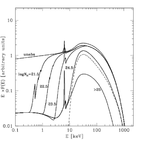
Figure 1: The AGN X-ray spectra with different absorptions assumed in the model. Solid lines from top to bottom: $N_{H}=0$ (i.e. unabsorbed AGN), log$N_{H}=21.5,22.5,23.5,24.5,>25$. A primary powerlaw with $\Gamma=1.9$ and cut off energy $E_{c}=200$ keV is assumed. A 3% soft scattered component is also added in the obscured AGN spectra. The spectrum of mildly Compton-thick AGN (log$N_{H}=24.5$) is obtained by summing a transmission component (dashed line) to the same reflection continuum used to model the spectrum of heavily ($logN_{H}>25$) Compton-thick AGN (see text). In each spectrum a 6.4 keV iron emission line is also added following Gilli et al. (1999a).

3.2 Obscured AGN

X–ray absorption by cold gas with column densities ranging from values ($N_{H}\lesssim 10^{21}$ cm^-2) barely detectable in the X–ray band to extremely large columns able to efficiently absorb the X–ray emission up to 10 keV ($N_{H}\gtrsim 10^{24}$ cm^-2) are routinely observed for both local (Risaliti et al. 1999) and distant AGN (Norman et al. 2002, Tozzi et al. 2006, Mainieri et al. 2005). For the sake of simplicity and following previous analysis (Comastri et al. 1995, Gilli et al. 2001) the absorbing column density distribution is parametrized with coarse, equally spaced, $\Delta logN_{H}$ = 1 bins centered at log$N_{H}$=21.5,22.5,23.5,24.5,25.5. The slope of the primary continuum is that of unobscured AGN with a lower reflection normalization (0.88 rather than 1.3). Indeed, if the accretion disk is aligned with the obscuring torus, the reflection efficiency for high inclination angles (expected for obscured AGN) is lower. A significant difference in the reflected component from the accretion disk in unobscured and obscured AGN is not yet seen in the data, however the typical values measured in samples of Seyfert 1s and Seyfert 2s are consistent with the assumed values (Risaliti 2002, Perola et al. 2002). As in the case of unobscured AGN, the disk reflection component was added only for sources at Seyfert-like luminosities.

The photoelectric absorption cut–off in Compton-thin AGN (log$N_{H}<24$) is computed using the Morrison & Mc Cammon (1983) cross sections for solar abundances, while absorption in the Compton-thick regime was computed with an upgraded version of a Monte Carlo code originally developed by Yaqoob (1997). As long as the absorption column density does not exceed values of the order of 10²⁵ cm^-2, the nuclear radiation above 10–15 keV is able to penetrate the obscuring gas. For higher column densities the X–ray spectrum is down-scattered by Compton recoil and hence depressed over the entire energy range. In the following we will refer to sources in the log$N_{H}=24.5$ and log$N_{H}=25.5$ absorption bins as “mildly Compton-thick”and “heavily Compton-thick” AGN, respectively. The broad band spectrum of mildly Compton-thick AGN is parametrized by two components: the transmitted one which dominates above 10 keV (dashed line in Fig. 1) and the reflected one which emerges at lower energies and is likely to be originated by reflection from the inner side of the obscuring torus. As for the relative normalization of the torus reflection component, which is only poorly known, we assumed a value of 0.37. This is such to produce a 2–10 keV reflected flux which is 2% of the intrinsic one and is consistent with the average ratio between the observed 2-10 keV luminosity of Compton-thick and Compton-thin AGN (see e.g. Maiolino et al. 1998a). A pure reflection continuum is assumed to be a good representation of the spectrum of heavily Compton-thick AGN over the entire energy range. As for the 6.4 keV iron emission line, a Gaussian with $\sigma=0.1$ keV was assumed for all obscured AGN, with equivalent width ranging from a few hundreds eV for moderately obscured sources to $\sim 2$ keV for Compton-thick objects (see details in Gilli et al. 1999a).

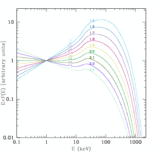
Figure 2: The spectral library assumed for unobscured Seyferts. Photon indices range from $\Gamma=1.5$ to $\Gamma=2.3$ in step of $\Delta\Gamma=0.1$. All the spectra are normalized at 1 keV.

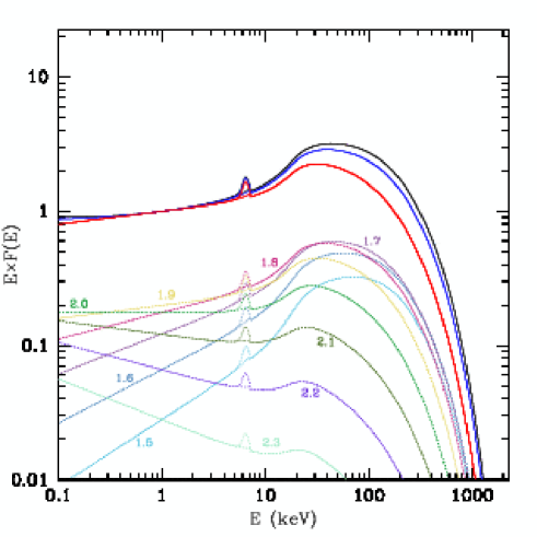
Figure 3: The effects of increasing the spectral dispersion $\sigma_{\Gamma}$ on the effective spectrum of unobscured AGN. The solid lines normalized at 1 keV correspond to the weighted sum over the assumed spectral distribution in the case of $\sigma_{\Gamma}$=0.0, 0.2 and 0.3 (from bottom to top curve, respectively). The case with null dispersion corresponds to assuming a single spectrum with $\Gamma=1.9$. The contribution of the individual spectra along the distribution (dotted lines with labeled photon index) is also shown for the $\sigma_{\Gamma}=0.2$ case. Note that at different energies the maximum contribution is provided by spectra with different slopes.

We finally added a soft component to the spectra of obscured AGN, since soft X-ray emission in excess of the absorbed powerlaw is common in the spectra of Seyfert 2 galaxies (e.g. Turner et al. 1997, Guainazzi & Bianchi 2006). The origin of this soft component has been proposed to be manifold: i) a circumnuclear starburst, which is often observed around the nuclei of Seyfert 2 galaxies (e.g. Maiolino et al. 1998b) ; ii) scattering of the primary powerlaw by hot gas (Matt et al. 1996); iii) leakage of a fraction of the primary radiation through an absorbing medium which covers only partially the nuclear source (Vignali et al. 1998, Malaguti et al. 1999); iv) sum of unresolved emission lines from photoionized gas (Bianchi et al. 2006a). Very recently Guainazzi & Bianchi (2006) have shown that, when observed with high spectral resolution, the soft X-ray emission of most Seyfert 2 galaxies can be explained as the sum of individual emission lines. However, since we are interested in the broad band properties of the X-ray spectrum, we keep a simple modeling of the soft X-ray spectrum by assuming a powerlaw with the same spectral index of the primary powerlaw. Following Gilli et al. (2001), the normalization of the scattered component was fixed to 3% of that of the primary powerlaw. This soft emission level is in agreement with the recent results mentioned above (Guainazzi & Bianchi 2006, see also Bianchi et al. 2006b).

The broad band spectral templates adopted in the calculations in the various absorption bins are shown in Fig. 1.

4 Dispersion of the photon indices

While it is well known since the first AGN spectral surveys (i.e. Maccacaro et al. 1988) that the distribution of X–ray spectral slopes is characterized by a not negligible intrinsic dispersion, this very observational fact has always been neglected in the synthesis of XRB spectrum. The most recent estimates (Mateos et al. 2005) from the analysis of relatively faint AGN in the Lockman Hole are consistent with an intrinsic dispersion of about 0.2–0.3 confirming previous results obtained for nearby bright Seyferts (Nandra & Pounds 1994). In the following we will discuss how the inclusion of a distribution of spectral slopes modifies the synthesis of the XRB spectrum with respect to the adoption of a single value.

It is easy to show that the spectrum obtained by averaging power law spectra with different slopes is different from that obtained computing the average slope :

$$\frac{1}{N}\sum_{i=1}^{N}\;E^{-\Gamma_{i}}\neq E^{-\langle\Gamma\rangle}.$$ (1)

We computed a set of unabsorbed AGN spectra with photon indices ranging from $\Gamma$=1.5 to 2.3, in step of $\Delta\Gamma=0.1$ to which we added the previously described (Section 3.1) spectral components. All the spectra are normalized at 1 keV and are shown in Fig. 2. We assumed that the spectral distribution is a Gaussian centered at $\Gamma=1.9$ and variable dispersion $\sigma_{\Gamma}$. Each spectrum with photon index $\Gamma_{i}$ was multiplied by the appropriate Gaussian weight $p_{i}$, i.e.:

$$p_{i}=\frac{1}{\sigma_{\Gamma}\sqrt{2\pi}}\int_{\Gamma_{i}-\Delta\Gamma/2}^{\Gamma_{i}+\Delta\Gamma/2}e^{-(\Gamma-\langle\Gamma\rangle)^{2}/2\sigma_{\Gamma}^{2}}{\rm d}\Gamma,$$ (2)

with

$$\sum_{i=1}^{N}\,p_{i}=1.$$ (3)

All the weigthed spectra were then summed together to produce an “effective” spectrum, which is shown in Fig. 3 as a function of the assumed dispersion $\sigma_{\Gamma}$.

The slope of the resulting spectrum hardens towards high energies for increasing values of the dispersion. By definition a null dispersion corresponds to a single power law with $\Gamma=1.9$. A dispersion of 0.2-0.3 produces an increase by 30-40% at energies above $\sim 30$ keV. Indeed, the relative contribution of the flatter slopes is higher at high energies, while the relative contribution of the steeper slopes is correspondingly increasing below 1 keV. As we will see later, the spectral hardening at high energies and especially around 30 keV due to the adopted dispersion has a significant impact on the XRB fit, affecting in turn the number of heavily obscured sources required to match the high energy XRB spectrum.

In addition to the distribution in the spectral indices we also considered the effects of a Gaussian distribution of the cut–off energy values, centered at $E_{c}=200$ keV and with variable dispersion encompassing the 50–500 keV energy range. The differences with respect to a single spectrum with zero dispersion are found to be very small, unless an extremely large dispersion corresponding to an almost flat distribution, is assumed. Even in that case, however, the deviations with respect to the zero dispersion case are observable only above 100–150 keV, and thus do not significantly alter our 30 keV XRB modeling. In the following we will therefore consider a single cut–off energy $E_{c}=200$ keV.

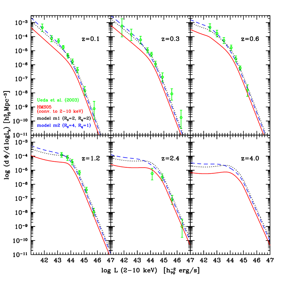
Figure 4: The Ueda et al. (2003) intrinsic hard XLF for the total Compton-thin AGN population (datapoints) compared with models m1 (dotted line) and m2 (dashed line). The soft XLF by HMS05 converted to the hard band is also shown (solid line). The XLF datapoints by Ueda et al. (2003) are limited to $z<3$.

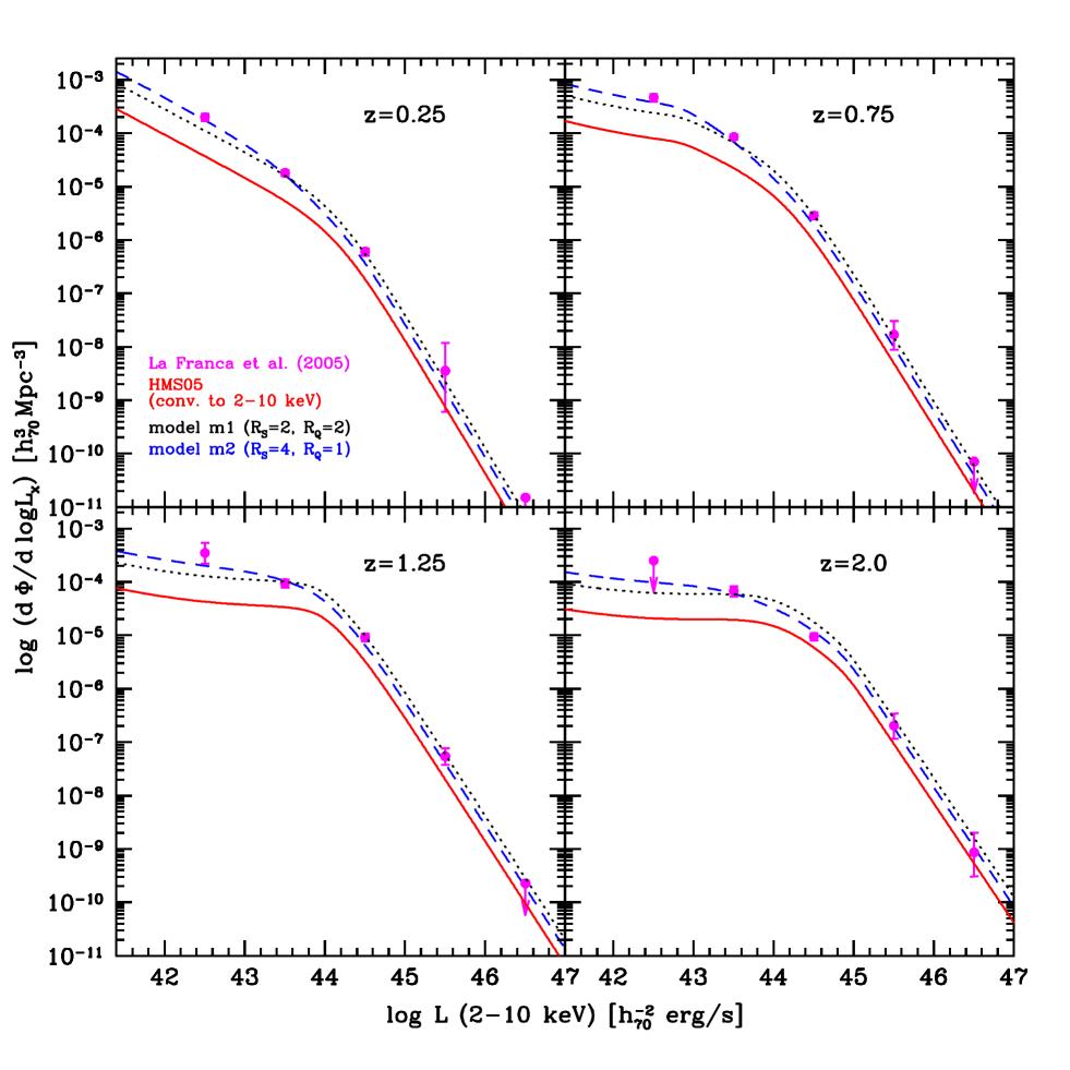
Figure 5: Same as the previous Figure but considering the hard XLF data of La Franca et al. (2005).

5 The XLFs and the obscured/unobscured AGN ratio

The accuracy in the determination of the AGN X-ray luminosity function parameters has significantly improved in the past few years, leading to a rather detailed knowledge of the AGN evolution up to redshifts of about 4. Besides the soft XLF, whose first reliable determinations date back to more than 10 years ago (Maccacaro et al. 1991; Boyle et al. 1994, Page et al. 1996), it has been recently possible to obtain a solid estimate of the AGN XLF also in the hard 2–10 keV band (Ueda et al. 2003, La Franca et al. 2005, Barger et al. 2005). It is worth noting that, although both the soft and hard X–ray selected sources are well described by a LDDE model, the dependence of the evolution rate with luminosity appears to be less extreme in the 2–10 keV band. This can already be regarded as an indication of a variable ratio between obscured and unobscured AGN as a function of luminosity and/or redshift as it will be shown later. Also, combining several AGN samples selected in the mid–infrared, optical blue band, soft and hard X–rays, Hopkins, Richards & Hernquist (2006) were able to compute the evolution of a ”bolometric” luminosity function (LF). A luminosity dependent density evolution (LDDE) model, where the evolution rate is higher for high-luminosity sources, combined with a decreasing fraction of obscured sources for increasing luminosities, provides a rather good description of AGN evolution over a wide range of frequencies, bolometric luminosities and redshifts.

As a reference XLF for our modeling we chose the most up-to-date calculation of Hasinger, Miyaji & Schmidt (2005, hereafter HMS05) in the 0.5–2 keV band, which is based on the largest number statistics (about 1000 objects) and spectroscopic completeness. It contains objects selected to have broad optical emission lines, or, when the quality of the optical spectra was poor, on the basis of their soft X-ray spectra (see HMS05 for details). It is known that about 10-20% of broad line AGN suffer from some X-ray absorption (e.g. Brusa et al. 2003, Georgantopoulos et al. 2004), as well as that soft X-ray spectra do not guarantee absence of absorption (especially for high-redshift objects, for which the absorption cut off may be shifted out of the observable X-ray band). Some contamination by obscured AGN is then likely to affect the soft XLF, but this cannot be easily sorted out and, at any rate, is not expected to alter significantly the LDDE parameters. In the following we will then consider the HMS05 XLF as a good approximation to the soft XLF of X-ray unobscured (log$N_{H}<21$) AGN.

While the soft XLF by HMS05 contains essentially unobscured AGN, the hard XLFs by Ueda et al. (2003) and La Franca et al. (2005) do not apply any pre-selection to the AGN included in their samples, which therefore contain both populations of obscured and unobscured AGN. Since both Ueda et al. (2003) and La Franca et al. (2005) measure the column density for each object in their sample (via a rough X-ray spectral analysis, often using hardness ratios), they can derive the intrinsic, de-absorbed luminosity for each source as well as the appropriate K-correction to the 2–10 keV rest frame band. They can therefore determine the intrinsic, rest frame 2–10 keV XLF, which is however dependent on the measured $N_{H}$ distributions, and may thus suffer from selection biases towards less obscured objects. We nonetheless consider the absorption corrections as a second order effect on the integral XLF, which in the following will be considered as independent on the measured $N_{H}$ distribution. The general agreement between the XLF by Ueda et al. (2003) and La Franca et al. (2003) despite the different $N_{H}$ distributions derived by these authors supports this assumption.

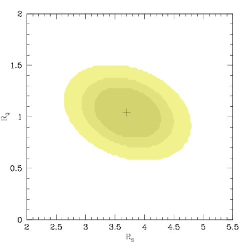
Figure 6: The 68,90,99% confidence contours on the best fit $R_{S}$ and $R_{Q}$ ratios computed for two interesting parameters ($\Delta\chi^{2}=2.3,4.61,9.21$, respectively).

While the population of Compton-thin AGN should have been sampled with a good accuracy level by the 2–10 keV surveys, heavily obscured Compton-thick sources, which, almost by definition, are extremely difficult to observe below 10 keV, should be essentially missing from the hard XLFs. We will therefore consider the 2-10 keV XLF by Ueda and La Franca as a good approximation to the 2-10 keV XLF of Compton-thin (log$N_{H}<24$) AGN. As a consequence, the XLF of moderately obscured AGN (21$<$log$N_{H}<$24) can be reasonably well estimated as the difference between the hard XLFs and the soft XLF by HMS05, once the latter is converted to the 2-10 keV band.

Since we assumed a distribution of spectra rather than a single powerlaw, we have to take into account different band corrections. We then split the soft XLF by HMS05 into 9 individual XLFs (as many as the considered spectral powerlaws). Each of them was then multiplied by the appropriate weight $p_{i}$ (see previous Section) and converted to the 2–10 keV band with the corresponding spectral index. The 2–10 keV converted individual XLFs were then summed together to produce the total hard XLF for unobscured sources. As shown in Fig. 4, this is not sufficient to match the XLF data by Ueda et al. (2003), and obscured AGN have to be added.

We introduce the ratio $R$ between obscured Compton-thin AGN and unobscured AGN (i.e. the number ratio between sources with $21<logN_{H}<24$ and with $logN_{H}<21$) defined as follows:

$$R(L)=R_{S}\;e^{-L/L_{c}}+R_{Q}\;(1-e^{-L/L_{c}}),\left\{\begin{array}[]{ll}R\rightarrow R_{S}\;\;\;(L<<L_{c})\\ R\rightarrow R_{Q}\;\;\;(L>>L_{c})\\ \end{array}\right.,$$ (4)

where $R_{S}$ is the ratio in the Seyfert (low-) luminosity regime and $R_{Q}$ is the ratio in the QSO (high-) luminosity regime, and $L_{c}$ is the 0.5–2 keV characteristic luminosity dividing the two regimes (we fixed $logL_{c}=43.5$). The total AGN hard XLF is simply obtained by converting the soft (unobscured) XLF to the hard band and then multiplying it by (1+$R(L)$).

We considered two hypotheses: first (model m1) a ratio independent of luminosity (i.e. $R_{Q}=R_{S}$); second (model m2), a variable ratio, where $R_{S}$ and $R_{Q}$ can vary independently.

We searched for the best fit $R_{S}$ and $R_{Q}$ values in model m1 and m2 by means of a $\chi^{2}$ test applied to the combined Ueda et al. (2003) and La Franca et al. (2005) datapoints. Model m1 is ruled out by the XLF comparison: the best fit ratio, $R_{S}=R_{Q}=1.6$ ($\chi^{2}/dof=94.8/50=1.9$) is rejected at $>99.99\%$ confidence level. On the contrary a model with a varying ratio, with best fit values $R_{S}=3.7$ and $R_{Q}=1.0$, provides a good match between the soft and hard XLF and is statistically acceptable ($\chi^{2}/dof=51.1/49=1.0$), strongly supporting previous observations of a declining ratio towards high intrinsic luminosities. We explored in some more detail the issue of a variable ratio, in particular trying to put some general constraints on the number of obscured QSOs. We checked if a model without obscured QSOs at all is a viable solution, by fixing $R_{Q}=0$ and leaving $R_{S}$ free to vary. The best fit solution ($\chi^{2}/dof=103/50=2.1$) is clearly unacceptable. Also, a large obscured QSOs fraction ($R_{Q}\geq 2$) does not provide an acceptable solution. In Fig. 6 we show the 68,90 and 99% confidence contours on $R_{S}$ and $R_{Q}$ computed for two interesting parameters ($\Delta\chi^{2}=2.3,4.61,9.21$, respectively; Avni 1976). In the following we will consider the 99% confidence intervals to quote uncertainties on the $R_{S}$ and $R_{Q}$ values. These rather conservative boundaries have been chosen to account for the uncertainties in the LDDE parametrization of the input XLF by HMS05, which should be also included in the error budget. The ratio $R_{Q}$ between obscured and unobscured QSOs is then constrained to be within 0.6 and 1.5. Similarly $R_{S}$ is constrained to be in the range 2.6-4.8. As we will show in the next Section a value of $R_{Q}\lesssim 1$ gives a better agreement with the obscured QSO fractions observed in different samples of 2-10 keV selected sources. In Fig. 4 and Fig. 5 we show the XLF comparison with model m1 (where we approximated $R_{S}=R_{Q}\sim 2$) and model m2 (where we approximated $R_{S}\sim 4$). We also verified if the $R_{S}$ and/or $R_{Q}$ values could increase with redshift, without finding any significant evidence. In the following we will consider model m2 with $R_{S}=4$ and $R_{Q}=1$ as our baseline model.

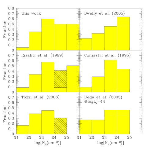
Figure 7: Comparison between the model $N_{H}$ distribution (upper left) and those obtained from previous works. The number of objects in each $N_{H}$ bin is normalized to the total number of Compton-thin ($21<{\rm log}N_{H}<24$) AGN, i.e. the sum of the first three $N_{H}$ bins is 1 (see Section 6 for details). The estimated fractions of Compton-thick objects are discussed in Sections 7 and 9. Shaded areas refer to lower limits to $N_{H}$.

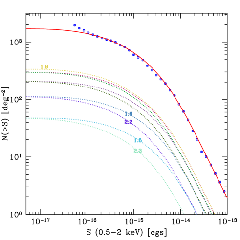
Figure 8: Cumulative soft AGN counts for unabsorbed AGN. An input distribution of photon indices with average=1.9 and dispersion=0.2 is assumed. The individual logN-logS for the different spectral classes (photon index is labeled for some of them), scaled by the corresponding weight along the distribution, are shown as dotted lines. The total logN-logS for unobscured AGN, resulting from the sum of the dotted lines, is shown as a solid line and is compared with the soft logN-logS measured for type-1 AGN by HMS05 (open circles).

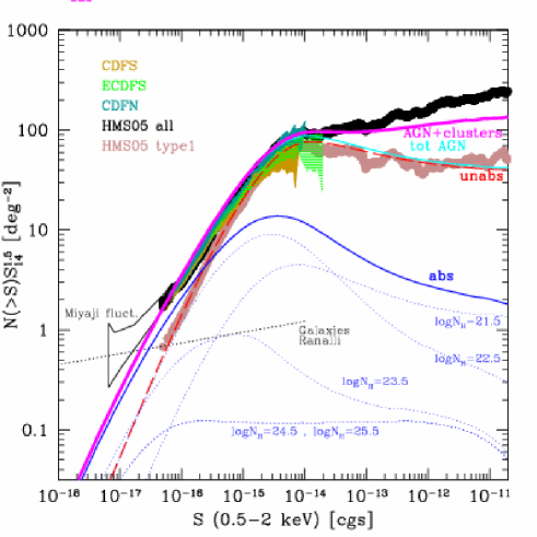
Figure 9: Cumulative soft AGN counts normalized to an Euclidean Universe. Datapoints are labeled on the top left: CDFS (Rosati et al. 2002); E-CDFS (Lehmer et al. 2005); CDFN (Alexander et al. 2003); compilation by Hasinger, Miyaji & Schmidt (2005) for all the 0.5-2 keV X-ray sources (HMS05 all) and type-1 AGN only (HMS05 type-1). The errorbox from the fluctuation analysis by Miyaji & Griffiths (2002) is also shown. The model curves for unabsorbed AGN, absorbed AGN, total AGN, and total AGN plus clusters are shown respectively with the following line styles: red long-dashed, blue solid, cyan solid, magenta solid. The logN-logS curves for individual $N_{H}$ classes are also shown as blue dotted lines. The curves for mildly (log$N_{H}=24.5$) and heavily (log$N_{H}=25.5$) Compton-thick AGN are fully described in Section 7. The total data by HMS05 are not cleaned by Galactic sources, thus producing an apparent discrepancy with respect to the total model prediction at bright fluxes. The logN-logS for normal galaxies by Ranalli et al. (2003) is also shown as a dotted straight line, which is expected to provide a significant contribution at very faint fluxes ($\lesssim 5\times 10^{-17}$ cgs).

6 Number counts and $N_{H}$ distribution

The comparison between the soft and hard XLF only constrains the total number of obscured Compton-thin AGN, but does not provide informations on their absorption distribution. The latter is estimated by considering the soft and hard cumulative number counts as explained below.

For each absorption class $j$ and slope $i$ individual logN-logS relations $N_{ij}(>S)$ were computed integrating the XLF of HMS05 in the $10^{42}-10^{48}$ erg s^-1 0.5-2 keV luminosity range and 0–5 redshift interval and taking into account the appropriate K-corrections. Besides the K-correction another correction has to be considered because of the shape of the effective area of X-ray imaging instruments, which is maximum at 1–2 keV and therefore favors the detection of sources with soft rather than hard spectral shapes. The correction method, described in detail in Gilli, Salvati & Hasinger (2001), is briefly recalled here. We considered the effective area of Chandra ACIS–I since many logN-logS, including the deepest ones, have been obtained with this instrument, and computed the count rate produced by sources with the same observed flux $S$ but different absorptions and redshifts $CR(N_{H},z)$. At any given flux $S$ the logN-logS relation for each absorption class was computed at an ”effective” flux $S(N_{H},z)=CR(\Gamma_{conv})/CR(N_{H},z)$, where $CR(\Gamma_{conv})$ is the count rate produced by a source with flux $S$ and with the X-ray spectrum originally used to derive the logN-logS measurement (i.e. to convert counts into fluxes). The net effect is then such that the number counts of obscured sources were computed at higher effective fluxes, thus mimicking the loss of instrumental sensitivity towards hard spectra.

Each individual logN-logS for unobscured AGN was then scaled by a factor $p_{i}$, where $p_{i}$ is the Gaussian weight for each spectral slope as defined in Eq. 2, while each individual logN-logS for obscured AGN was scaled by a factor

$$f_{ij}=p_{i}\,R(L)\,d_{j},$$ (5)

where $R(L)$ is the Compton-thin to unabsorbed AGN ratio defined in Eq. 4 and $d_{j}$ is the fraction of obscured AGN in each of the three Compton-thin classes log$N_{H}$=21.5,22.5,23.5, such that

$$\sum_{j=1}^{3}d_{j}=1$$ (6)

Since a flat $N_{H}$ distribution was found to overestimate the soft counts, we assumed that the factor $d_{j}$ is increasing with obscuration from $logN_{H}=21.5$ to $logN_{H}=23.5$. A similar increase has been actually observed by several authors using different data-sets (e.g. Risaliti et al. 1999, Dwelly et al. 2005, Tozzi et al. 2006) and already assumed in previous synthesis models (Comastri et al. 1995, Gilli et al. 2001).

The considered $N_{H}$ distribution is shown in Fig. 7, together with other $N_{H}$ distributions from the literature. It is worth noting that all of these distributions are intrinsic, i.e. those which would be observed at extremely low (formally zero) limiting fluxes.

With such an approach our model provides quantitative and accurate predictions on both the $N_{H}$ and $\Gamma$ distribution to be observed at any given limiting flux, thus allowing comparisons with the numerous results obtained by recent X-ray surveys as discussed in Section 8.

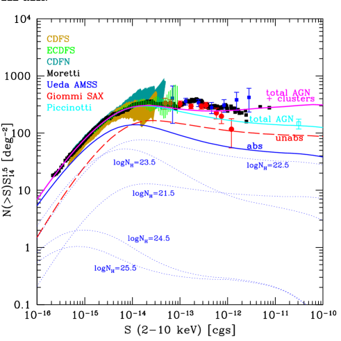
Figure 10: Cumulative 2-10 keV AGN counts normalized to an Euclidean Universe. The model curves and corresponding line styles are the same as in Fig. 9 and are compared with datapoints from different surveys: CDFS (Rosati et al. 2002); E-CDFS (Lehmer et al. 2005); CDFN (Alexander et al. 2003); the Moretti et al. (2004) compilation; ASCA Medium Sensitivity Survey (AMSS, Ueda et al. 2001); BeppoSAX 2-10 keV survey (Giommi et al. 2002); HEAO-1 A2 all sky survey (Piccinotti et al. 1982). The logN-logS curves for mildly (log$N_{H}=24.5$) and heavily (log$N_{H}=25.5$) Compton-thick AGN are fully described in Section 7.

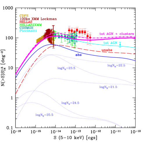
Figure 11: Cumulative 5-10 keV AGN counts normalized to an Euclidean Universe. The model curves and corresponding line styles are the same as in the previous figures and are compared with datapoints from different surveys: CDFS (Rosati et al. 2002); 100 ks Lockman Hole (Hasinger et al. 2001); BeppoSAX HELLAS (Fiore et al. 2003); HELLAS2XMM (Baldi et al. 2002); COSMOS (Cappelluti et al. 2006); HEAO-1 A2 all sky survey (Piccinotti et al. 1982) converted to the 5-10 keV band. The logN-logS curves for mildly (log$N_{H}=24.5$) and heavily (log$N_{H}=25.5$) Compton-thick AGN are fully described in Section 7. The dot-dashed line is the total model prediction when assuming an average spectral index of $\langle\Gamma\rangle=1.8$ (see the Discussion).

As shown in Fig. 7 the $N_{H}$ distribution considered in this work contains a very low fraction of AGN obscured by column densities in the range $21<logN_{H}<22$. While this may appear unrealistic, it should be noted that about 10% to 20% of the sources in the HMS05 type-1 AGN catalog, which here are assumed to be unobscured, may belong to the class of mildly obscured 21$<logN_{H}<$22 AGN. Absorbing column densities in this range may well have escaped detection especially if at moderate to high redshifts. These AGN would mostly “fill in” the $logN_{H}=21.5$ bin, thus making the steep rising towards high columns less extreme than that shown in Fig. 7. If this is the case, the ratio between obscured and unobscured AGN determined in the previous Section would increase by $\sim 20-30\%$.

In Fig. 8 we show the individual 0.5-2 keV logN-logS for the unobscured AGN population, each scaled by the appropriate factor $p_{i}$ as a function of different spectral slope, where the effects of the different K-corrections for the different slopes can be fully appreciated. As an example, sources with $\Gamma=1.5$ and $\Gamma=2.3$, which are weighted by the same factor $p_{i}$ for a Gaussian distribution centered at $\langle\Gamma\rangle$=1.9, provide an equal contribution at very faint fluxes (as it should be expected since at very faint fluxes all the sources in the XLF can be detected), while at bright fluxes objects with $\Gamma=1.5$ are observed more easily due to their stronger K–correction.

The 0.5–2 keV AGN counts resulting from our baseline model m2 are shown in Fig. 9, where we plot the logN-logS relation scaled by $S_{14}^{1.5}$ (where $S_{14}$ is the flux in units of $10^{-14}$ erg cm^-2 s^-1) to expand the scale on the y-axis and facilitate the evaluation of any difference between the data and the model. The source counts for unobscured and Compton-thin AGN as well as the total are shown. In addition, we also computed the contribution from galaxy clusters following Gilli et al. (1999b). From an observational point of view, the logN-logS relation in the soft band is now measured over a flux range encompassing more than 6 orders of magnitude (HMS05). A compilation from surveys at different limiting fluxes is shown in Fig. 9. The model logN-logS is found to reproduce with excellent accuracy the source counts over the whole flux range with the exception of very bright and very faint fluxes. This has however to be expected since X–ray sources other than AGN contribute in those regimes: at bright fluxes ($S>10^{-13}$ cgs) the total logN-logS by HMS05 includes also galactic sources (therefore the total model logN-logS – AGN plus clusters – underestimates the observed counts); at very faint fluxes ($\lesssim 5\,10^{-17}$ cgs) a population of normal and star forming galaxies is expected to contribute significantly to the total counts (see e.g. Ranalli et al. 2003). The galaxy logN-logS predicted by Ranalli et al. (2003) is also plotted in Fig. 9

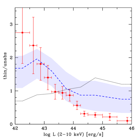
Figure 12: The observed ratio between optical type-2 and type-1 AGN in the Hasinger (2006) sample as a function of intrinsic 2-10 keV luminosity compared with ratio between obscured (log$N_{H}>21$) and unobscured (log$N_{H}<21$) AGN as predicted by model m2 (dashed line) and m1 (dotted line) after folding with the appropriate selection effects of the observed sample. The shaded area represent the uncertainties on model m2. Model m1 (constant intrinsic ratio) appears strongly disfavored.

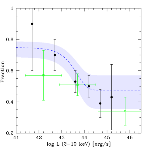
Figure 13: The intrinsic fraction of AGN with log$N_{H}>22$ vs intrinsic 2-10 keV luminosity as determined by Akylas et al. (2006, filled circles) and Ueda et al. (2003, open squares) compared with the corresponding fraction assumed in model m2 (dashed line). Uncertainties on model m2 are shown by the shaded area.

We then checked the model expectations against the source counts in the harder 2–10 keV and 5–10 keV bands. The results are shown in Fig 10 and Fig 11, respectively, where we also plot the individual curves for absorbed and unabsorbed AGN, total AGN and total AGN plus galaxy clusters. At fluxes above $\sim 10^{-13}$ cgs galaxy clusters provide a significant contribution both in the 2-10 keV and 5-10 keV bands. The datapoint at $\sim 3\,10^{-11}$ cgs represents the surface density of AGN in the Piccinotti et al. (1982) sample, which is well matched by the model curve representing AGN alone. While both the 0.5–2 keV and the 2–10 keV source counts are well reproduced over several orders of magnitude in flux, in the 5–10 keV band the model predictions appear in good agreement with the observations in the flux range covered by the HELLAS2XMM (Baldi et al. 2002) and COSMOS (Cappelluti et al. 2006) surveys, but, on average, lay slightly below the available measurements (although within 1-2$\sigma$). The very hard 5–10 keV counts are almost perfectly fitted assuming a slightly harder average spectrum ($\langle\Gamma\rangle=1.8$; see Fig. 11). However, it is likely that non-negligible systematic uncertainties affect the logN–logS of sources detected in the narrow 5–10 keV band where the instrumental sensitivity rapidly falls off. We will return on this point in the Discussion.

Once the total number and $N_{H}$ distribution of the Compton-thin AGN population have been fixed, we can now predict the fraction of obscured AGN at different fluxes and in different luminosity bins and compare it with the observations. In particular we considered the compilation of 2–10 keV selected AGN by Hasinger (2006 in preparation; see also Hasinger 2004), who combined the data from surveys of different areas and limiting fluxes to get a sample of $\sim 700$ objects. In Fig.12 we show the ratio between optical type-2 and type-1 AGN as a function of their intrinsic 2–10 keV luminosity as obtained by Hasinger (2006), compared with the expectations of models m1 and m2 folded with an appropriate sensitivity curve to account for the selection effects in the observed sample. In model m1, where the ratio between obscured and unobscured sources is constant, the $observed$ ratio appears to increase towards higher luminosities, since obscured sources of low intrinsic luminosity are the first to be missed in flux limited samples. In model m2 the observed trend is reversed with respect to model m1 because the above mentioned effect is compensated by the intrinsically higher ratio at low luminosities. As it is evident, model m1 is in stark contrast with the observations, while model m2 produces a much better agreement, although the model predictions are on average slightly higher than the data. We note that several uncertainties affect the comparison shown in Fig. 12: first of all the sensitivity curve adopted to get the model predictions is just an approximation to the full sky coverage of the Hasinger (2006) sample; then comparing an optical type-2/type-1 ratio with an X-ray obscured to unobscured AGN ratio always suffers from limitations related to the AGN classification in different bands; finally a $\sim 20\%$ degree of spectroscopic incompleteness is present in the considered sample. Therefore, we do not try to accurately reproduce the observed fractions but we use this plot to further rule out model m1.

The decreasing obscured AGN fraction towards high luminosities assumed in model m2 is also in good agreement with the very recent determinations of Akylas et al. (2006) who combined a number of shallow XMM pointings with the Chandra Deep Field South data to derive the intrinsic fraction of obscured AGN as a function of their intrinsic 2–10 keV luminosity. As shown in Fig.13, the fraction of AGN with log$N_{H}<22$ found by Akylas et al. (2006) is well matched by our baseline model m2 (the same fraction as measured by Ueda et al. 2003 is also reported in the plot.)

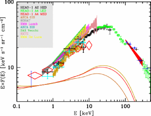
Figure 14: The integrated contribution of unobscured AGN to the XRB spectrum as a function of the dispersion in their spectral distribution ($\sigma_{\Gamma}$). From bottom to top curve: $\sigma_{\Gamma}$ = 0.0, 0.2, 0.3. The spectral distribution is centered at $\langle\Gamma\rangle=1.9$. Datapoints are explained in detail in the Caption of Fig. 15.

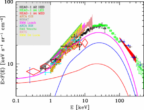
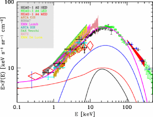
Figure 15: (a): The cosmic XRB spectrum and predicted contribution from the population of Compton-thin AGN. The different XRB measurements are explained on the top left: different instruments on board HEAO-1 (Gruber 1992, Gruber et al. 1999); ASCA GIS (Kushino et al. 2002); ROSAT PSPC (Georgantopoulos et al. 1996); two different measurements by XMM (Lumb et al. 2002, De Luca & Molendi 2003); ASCA SIS (Gendreau et al. 1995); BeppoSAX (Vecchi et al. 1999); RXTE (Revnivtsev et al. 2003). At $E>100$ keV the plotted datapoints are from HEAO-1 A4 MED (red triangles: Gruber 1992, Gruber et al. 1999; shaded area: Kinzer et al. 1997); balloon experiments (blue triangles, Fukada et al. 1975); SMM (green circles, Watanabe et al. 1997). The blue errorbar at 0.25 keV is from shadowing experiments by Warwick & Roberts (1998). Also shown are the XRB fractions resolved by Worsley et al. (2005) in the Lockman Hole (red diamonds), CDFS (cyan crosses) and CDFN (black crosses). The resolved fraction in the CDFS as measured by Tozzi et al. (2001a) is also shown (gold datapoints). Solid lines refer to the contribution of different AGN classes according to model m2. Unobscured AGN, obscured Compton-thin AGN, total AGN plus galaxy cluster are shown with a red, blue and magenta curve, respectively. (b): same as the previous panel but including also the contribution of Compton-thick AGN (black line).

7 The XRB spectrum

Having obtained a robust description of the unobscured and Compton-thin AGN properties – in particular of their relative ratio and absorption distribution – making use of the soft and hard XLF and logN–logS, their contribution to the XRB spectrum can be readily computed. As in the case of the logN-logS relations, we computed the contribution from each individual spectral and absorption class using the appropriate weight as given by Eq. 5, and then summed all of them together. Consistently with the computation of the source counts (see Section 6), the input XLF of HMS05 is integrated in the $10^{42}-10^{48}$ erg s^-1 0.5-2 keV luminosity range and 0–5 redshift interval.

In order to quantify the effects of an intrinsic dispersion in the spectral slope distribution we show in Fig. 14 the contribution of only unobscured AGN. Increasing the dispersion from zero to 0.2 and 0.3, the contribution at 30–40 keV is increased by 30–40%. This has the obvious consequence of reducing the number of obscured sources required to match the XRB peak intensity.

The effects of the dispersion in the photon indices is considered also when computing the contribution of the absorbed Compton-thin population. In Fig. 15a we show the separate contribution to the XRB spectrum from unobscured and obscured Compton-thin AGN as well as their summed contribution. The total curve also includes the contribution from galaxy clusters (which is at most $\sim 10\%$ at 1 keV; see Gilli et al. 1999b).

The integrated emission from the considered populations reproduces the entire resolved XRB flux (e.g. Worsley et al. 2005) up to 5–6 keV, while in the 6–10 keV range it is slightly above it. In other words, the deepest X–ray surveys have already sampled the whole unobscured and most of the obscured Compton-thin population. Also, Compton-thin AGN are found to explain most of the XRB below 10 keV as measured by HEAO-1 A2, but fail to reproduce the 30 keV bump, calling for an additional population of Compton-thick objects. We then added as many Compton-thick AGN as required to match the XRB intensity above 30 keV, under the assumptions that the number of mildly Compton-thick objects (log$N_{H}$=24.5) is equal to that of heavily Compton-thick objects (log$N_{H}$=25.5), as observed in the local Universe (Risaliti et al. 1999), and that they have the same cosmological evolution of Compton-thin AGN. The fit requires a population of Compton-thick AGN as numerous as that of Compton-thin ones, i.e. four times the number of unobscured AGN at low luminosities and an equal number at high luminosities. With Compton-thick AGN the total obscured to unobscured AGN ratio decreases from 8 at low luminosities to 2 at high luminosities. It is worth noting that the above ratio is estimated by fitting the XRB level at 30 keV as measured by HEAO1–A2. The global fit to the XRB spectrum is shown in Fig. 15b. Since the HEAO-1 A2 background is found to be lower by about 20% with respect the most recent determinations of the 2–10 keV background intensity (Kushino et al. 2002, Lumb et al. 2002, Hickox & Markevitch, 2006), our model does not account for the full XRB values measured by e.g. ASCA, XMM and Chandra. We will address the issue of the XRB spectral intensity in the Discussion.

Having constrained the space density of Compton-thick AGN with the fit to the XRB, the source counts in the 0.5–2 keV, 2–10 keV and 5–10 keV can be computed for the entire AGN population. Although Compton-thick AGN provide a measurable contribution only at very faint fluxes (see Figs 9,10,11), it is interesting to look at the behaviour of their logN-logS in more detail. In the soft band (see Fig.9) the curves for mildly and heavily Compton-thick AGN coincide since i) their space density is the same and ii) they have the same K-correction. Indeed, since the spectrum of mildly and heavily Compton-thick AGN is the same (reflection dominated) up to $\sim 10$ keV (see Fig.1), the 0.5-2 keV band is sampling an identical continuum even for sources at high redshift (up to $z\sim 4$). In the 2–10 keV and 5–10 keV band instead the curves for mildly Compton-thick and heavily Compton-thick sources show significant differences: at very bright fluxes, above $\sim 10^{-12}$ cgs, where only local sources are visible, the logN-logS curves of the two Compton-thick classes coincide because in the 2–10 keV rest frame band their spectrum is dominated by the same reflection continuum (Fig. 1). On the contrary, at fainter fluxes, $\sim 10^{-14}-10^{-15}$ cgs, where more distant sources can be detected, the surface density of mildly Compton-thick AGN appears about twice that of heavily Compton-thick AGN because of the stronger K-correction produced by the transmitted continuum (Fig .1).

8 Additional constraints

8.1 The observed fractions of obscured and Compton-thick AGN

There is strong evidence, obtained combining deep and shallow surveys over a broad range of fluxes, of an increasing fraction of obscured AGN towards faint fluxes (see e.g. Piconcelli et al. 2003). This general trend was expected and predicted by AGN synthesis models. However, the very steep increase in the observed ratio from bright to faint fluxes is poorly reproduced by models where the obscured to unobscured AGN ratio does not depend on X–ray luminosity (see Comastri 2004 for a review), while it is best fitted by assuming that the obscured AGN fraction increases towards low luminosity and/or high redshifts (La Franca et al. 2005).

We compare the observed fraction of AGN with log$N_{H}>22$ with the model predictions in Fig. 16. The choice of an absorption threshold at log$N_{H}>22$ rather than at log$N_{H}>21$ provides a more solid observational constraint, given the uncertainties in revealing mild absorption in sources at moderate to high redshift and/or with low photon statistics (Tozzi et al. 2006, Dwelly et al. 2005). The model curve is able to reproduce the steep increase of the absorbed AGN fraction from about 20–30% at $\lesssim 10^{-13}$ cgs, i.e. at the flux level of ASCA and BeppoSAX medium sensitivity surveys, to 70-80% as observed at $5\,10^{-15}$ cgs in the deep Chandra fields. Recently, Tozzi et al. (2006) performed a detailed X-ray spectral analysis of the CDFS sources, identifying 14 objects, i.e. about 5% of the sample, as likely Compton-thick candidates. As shown in Fig.16, this measurement is found to be in excellent agreement with the fraction of Compton-thick AGN predicted by our model at that limiting flux. These results confirm that below 10 keV the large population of Compton-thick sources is poorly sampled even by the deepest surveys.

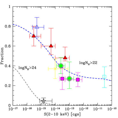
Figure 16: The fraction of obscured AGN observed in different X-ray surveys as a function of 2-10 keV limiting flux compared with the model predictions. The upper (lower) curve and datapoints refer to the fraction of obscured AGN with log$N_{H}>22$ (log$N_{H}>24$). Datapoints have been collected from the CDFS (open triangle and star, Tozzi et al. 2006), CDFN (filled triangles, Barger et al. 2005), XMM-Lockman Hole (cross, Mainieri et al. 2002), HELLAS2XMM (filled circles, Perola et al. 2004), Piconcelli et al. (2003) sample (filled squares), Piccinotti et al. (1982) sample (open square). The $N_{H}$ measurements for the Piccinotti et al. (1982) sample have been drawn from Shinozaki et al. (2006).

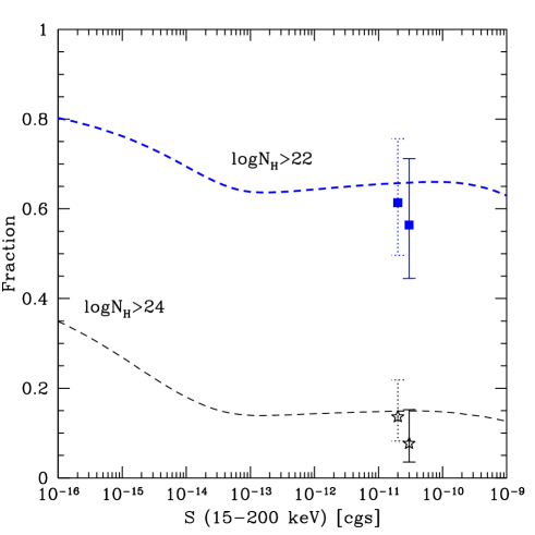
Figure 17: The fraction of obscured sources as a function of the 15-200 keV limiting flux predicted by the baseline model m2. The upper and lower curves refer to the fraction of objects with log$N_{H}>22$ and log$N_{H}>24$, respectively. Datapoints show the corresponding fractions found in the first Swift/BAT AGN catalog. While the datapoints with solid errorbars show the actually measured fraction, datapoints with dotted errorbars assume that most of the unidentified sources are obscured.

Very recently the first statistically well defined samples of AGN selected at energies above 10 keV have become available. The first release of AGN catalogs detected by the IBIS (20–100 keV band) and ISGRI (20–40 keV band) instruments on board INTEGRAL (Bird et al. 2006; Beckmann et al. 2006) includes about 40-60 objects. At the bright fluxes sampled by INTEGRAL (a few times $10^{-11}$ cgs in the 20-40 keV band), about two thirds of the identified AGN are absorbed by a column density in excess of log$N_{H}>22$ and about 10-15% have been found to be Compton-thick (Beckmann et al. 2006; Bassani et al. 2006). While the quoted fractions should be taken with the due care since the INTEGRAL AGN samples are still incomplete, they nonetheless are in good agreement with those measured at similar fluxes and for a similar waveband (15–200 keV) in the first Swift/BAT AGN catalog (Markwardt et al. 2006), which on the contrary is about 90% complete.

By considering the X-ray properties of the unidentified sources, the number of Compton-thick AGN in the first Swift/BAT catalog is estimated to be between 3 and 6, which translates into a fraction of 7-14%.

We computed the logN-logS relations expected from our baseline model m2 in the Swift/BAT band, as well as the expected fractions of obscured sources. At a limiting flux of $3\,10^{-11}$ cgs in the 15-200 keV band, i.e. the limiting flux of the BAT AGN catalog, about 65% of the AGN are obscured by log$N_{H}>22$ and about 15% are Compton-thick, in excellent agreement with the observations (see Fig. 17).

8.2 Spectral distribution

An interesting feature of having assumed a spectral index distribution is that the expected average spectral index is a function of the survey limiting flux. This can be easily understood by looking at Fig. 8, where the logN-logS for unobscured AGN with different spectral slope is plotted. Due to the different K-corrections, at bright X-ray fluxes sources with harder spectrum are detected more easily, while at fainter fluxes, where most of the sources in the XLF are being sampled, the observed distribution approaches the assumed, intrinsic one. In Fig. 18 we show the spectral distribution expected at different 2-10 keV fluxes for unobscured AGN. While at fluxes below $10^{-13}$ cgs the average expected slope is $\Gamma=1.7-1.8$, the spectral distribution progressively moves towards steeper values at fainter fluxes, until it exactly overlaps with the assumed input one at very faint fluxes $\sim 10^{-17}$ cgs.

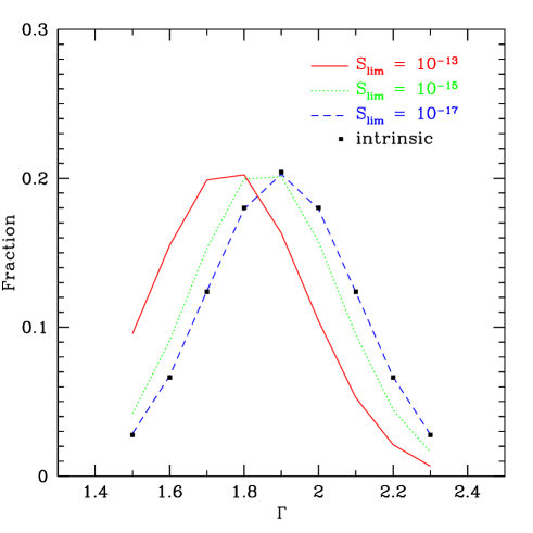
Figure 18: The spectral distribution of unobscured AGN to be observed at different 2-10 keV limiting fluxes as predicted by model m2. At very faint fluxes ($\sim 10^{-17}$ cgs) all the sources can be detected and the observed distribution coincides with the intrinsic one (filled squares) with $\langle\Gamma\rangle=1.9$ and $\sigma_{\Gamma}=0.2$.

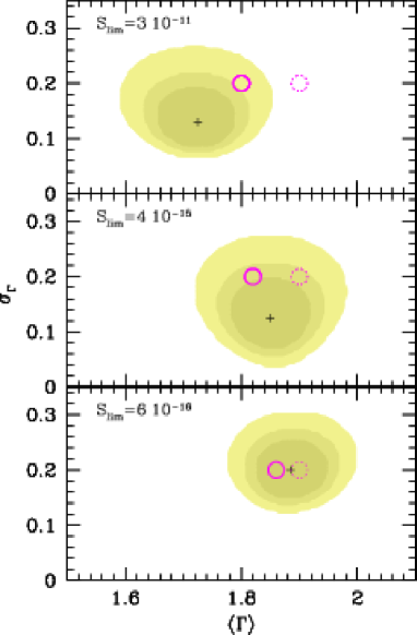
Figure 19: The average photon index and intrinsic dispersion measured in different samples of type-1 AGN (shaded areas; from top to bottom: Shinozaki et al. 2006, Tozzi et al. 2006, Mateos et al. 2005), compared with the model predictions for unobscured AGN (solid circles) at the corresponding 2-10 keV limiting fluxes (upper left labels). Only sources with good photon statistics have been considered. The different contours refer to the 68,90 and 99% confidence level for two interesting parameters ($\Delta\chi^{2}=2.3,4.61,9.21$, respectively) around the best fit values (crosses). Contours in the lower panel have been adapted from Mateos et al. (2005). The dotted circles represent the intrinsic (i.e. at zero flux) average photon index and dispersion assumed in the model.

This expected trend can be checked against the properties of sources detected in surveys at different limiting fluxes, provided that the photon statistics in the observed X-ray spectra is sufficiently high to provide a good estimate of the spectral slope. The X-ray spectral sample presented by Mateos et al. (2005) for AGN detected at 2-10 keV fluxes above $\sim 6\,10^{-16}$ cgs in the 800 ksec XMM-Lockman Hole satisfies this requirement since all AGN in their sample have been selected to have at least 500 X-ray counts in the 0.2-12 keV band. To reduce at minimum the uncertainties on the spectral slopes which, for sources with the same photon statistics, are larger for absorbed X-ray spectra due to the correlation between absorption and powerlaw index, we considered only the 46 type-1 AGN in Mateos et al. (2005), for which they measure an average spectral slope of $\Gamma=1.89\pm 0.06$ with an intrinsic dispersion of $\sigma_{\Gamma}=0.20\pm 0.04$ (see their Table 4) using the maximum likelihood method described by Maccacaro et al. (1988). We also considered two additional source samples at different fluxes. First we considered the CDFS sample by Tozzi et al. (2006), by selecting only spectroscopically confirmed type-1 AGN with more 500 X-ray counts. A total of 22 sources were selected in this way, with 2-10 keV fluxes above $4\,10^{-15}$ cgs. Then, at much brighter fluxes we considered the sample presented by Shinozaki et al. (2006) who analyzed the X-ray spectra, mainly obtained with XMM, of the Piccinotti et al. (1982) sample. This includes 17 type-1 AGN detected by HEAO-1 A2 at 2-10 keV fluxes above $3\,10^{-11}$ cgs, for which even short XMM exposures provide good quality data and allow a careful spectral analysis. For both samples we computed the average photon index and dispersion using the same Maximum Likelihood method described by Maccacaro et al. (1988). The results, combined with those obtained by Mateos et al. (2005) and compared with the model predictions for unobscured AGN at the same limiting fluxes, are shown in Fig. 19. The average steepening of the unobscured AGN slope towards faint X-ray fluxes predicted by the model appears to be in good agreement with the observations. It is worth stressing that the above described steepening of the intrinsic source spectra towards faint fluxes is due to the assumption of an intrinsic dispersion of the average power law slopes and is by no means in contrast with the flattening of the average slope observed in deep fields (Tozzi et al. 2001b). The latter is the result of fitting with a single power law the spectra of obscured sources and is ruled by their increasing contribution towards faint fluxes.

9 Discussion

The results of the self-consistent XRB modelling presented in the previous sections have been obtained under several, though observationally justified, assumptions. In the following we will further explore the parameter space in order to strengthen the model predictive power especially for what concerns the population of Compton-thick AGN.

9.1 Exploring the parameter space

The choice of a distribution of AGN X–ray spectra with an average slope $\langle\Gamma\rangle=1.9$ and dispersion $\sigma_{\Gamma}$=0.2, though consistent with the observations of bright AGN, may not necessarily hold over the broad range of redshifts and luminosities here considered. In the following it will be shown that, within the basic model assumptions, the average photon index is tightly constrained to be in the range $1.8<\langle\Gamma\rangle<2.0$. As a first step we checked the effects of a different value for the average photon index. Since in soft X–ray surveys an average slope of $\langle\Gamma\rangle\sim 2$ is observed, we considered a distribution centered at $\langle\Gamma\rangle=2$ (still having dispersion 0.2). Since the average unobscured AGN spectrum is now softer, the flux ratio between the 2–10 keV and the 0.5–2 keV band is lower and, as a consequence, more obscured AGN have to be added to match the hard XLF of Ueda et al. (2003) and La Franca et al. (2005). In particular, the $R_{S}$ and $R_{Q}$ values have to be increased from 4 to 5 and from 1 to 2, respectively. This larger number of obscured Compton-thin sources, however, violates the limits imposed by the observed number counts in the 0.5–2 keV band. Indeed, beyond the limits of shallow soft X–ray surveys, these obscured sources emerge at faint fluxes due to the favorable K–correction overproducing the observed counts. On the contrary, a spectral distribution centered at $\langle\Gamma\rangle=1.8$ implies a lower number of obscured AGN required to match the hard XLF and the XRB spectrum, and turns out to be in agreement with the source counts in all the considered bands. In particular, as shown in Fig. 11, assuming $\langle\Gamma\rangle=1.8$ would help in matching the 5–10 keV counts as observed in the HELLAS and CDFS surveys, which are otherwise slightly underestimated when $\langle\Gamma\rangle=1.9$. While improving the fit of the very hard counts, the choice of an harder ($\langle\Gamma\rangle=1.8$) spectrum brings a drawback: the average spectrum at various limiting fluxes does not match the observed one anymore (e.g. Mateos et al. 2005). One may then wonder whether the model should better reproduce the very hard 5–10 keV counts or the average spectra at faint X–ray fluxes. In this respect we note that the source detection in the 5–10 keV band and the corresponding logN–logS determination suffer from systematic calibration uncertainties much larger than those affecting the broader and softer 0.5–2 keV and 2–10 keV bands, mainly because the XMM-Newton, Chandra and BeppoSAX effective areas above 5 keV are rapidly decreasing. It is also worth mentioning that keeping the dispersion at $\sigma_{\Gamma}$=0.2 the harder average spectrum implies that the 30 keV XRB peak intensity (as measured by HEAO1) can be successfully reproduced without including any contribution from Compton-thick AGN. On the basis of what discussed above we feel that the slight underprediction of the very hard counts in the baseline model with $\langle\Gamma\rangle=1.9$ and $\sigma_{\Gamma}$=0.2 should not be considered a major inconsistency.

Then the effects of varying the width $\sigma_{\Gamma}$ of the spectral distribution were considered. If we assume a very narrow distribution, for instance $\sigma_{\Gamma}$=0, corresponding to a single $\Gamma=1.9$ photon index, the model predictions for the 0.5–2 keV and 2–10 keV observational constraints are essentially the same as those of the baseline model m2. Indeed, as shown in Figs. 3 and 14, the effects introduced by a distribution of spectral slopes increase towards high energies: the wider is the slope distribution the larger is the contribution to the XRB at say 30 keV (see Fig. 14). Therefore, the spectral dispersion $\sigma_{\Gamma}$ and the space density of Compton-thick sources are tightly correlated quantities. Assuming a distribution with $\sigma_{\Gamma}$=0, the contribution of Compton-thin sources to the 30 keV is lower than in our baseline model m2 and a larger number of Compton-thick sources has to be added to match the XRB broad band spectrum. More specifically one has to add twice as many Compton-thick sources as in model m2. This possibility appears to already overestimate the number of Compton-thick objects in the first BAT and INTEGRAL AGN surveys above 20 keV.

The high energy cut–off in the AGN spectra is very poorly constrained by present observations. The choice of $E_{c}$=200 keV in the adopted spectral templates for both unobscured and obscured AGN is basically driven by the intensity and the shape of the XRB spectrum above the peak, which cannot be exceeded. Assuming a cut off energy $E_{c}=300$ keV, leaving the mean and dispersion of the photon index distribution unchanged (1.9 and 0.2, respectively), the contribution of unobscured and Compton-thin AGN saturate the XRB emission at 100 keV but underestimate the 30 keV peak by about 20%. When trying to add Compton-thick sources to fit the 30 keV emission, the XRB at 100 keV is then overestimated. A global fit to the XRB spectrum using $E_{c}=300$ keV can still be achieved but, in order to reduce the model prediction at 100 keV with respect to that at 30 keV, one has to assume a null dispersion in the photon index distribution, which appears at variance with what discussed above. It is concluded that the average cut-off energy cannot be much higher than $E_{c}=200$ keV especially if AGN X–ray spectral slopes are characterized by some intrinsic dispersion. More detailed considerations on the average value of $E_{c}$ and the XRB constraints will be subject of future work and will not be addressed here.

Very recently Hao et al. (2005) derived the optical luminosity function of local low luminosity Seyferts, showing that their number density is still increasing down to absolute magnitudes $M_{B}\simeq$ –16 to –14, which roughly correspond to log$L_{x}\lesssim 41$ assuming standard AGN spectral energy distributions (e.g. Vignali et al. 2005). We then explored the effects of extrapolating the HMS05 XLF faint end slope down to log$L_{x}=41$, i.e. below the observational limit of log$L_{x}=42$ which has been assumed in our calculations. The predicted 0.5–2 keV counts of unabsorbed AGN exceed those observed by HMS05 for type-1 AGN at faint fluxes ($<10^{-16}$ cgs). This suggests that at low luminosities the slope of the AGN XLF should be flatter than that observed at log$L_{X}>42$.

9.2 The evolution of the fraction of obscured AGN with luminosity and redshift

The evidence for a decrease in the fraction of obscured objects at high X–ray luminosities is rapidly growing (Ueda et al. 2003, Hasinger 2004, La Franca et al. 2005, Akylas et al. 2006), confirming the early suggestion of Lawrence & Elvis (1982). Further evidences supporting a decreasing fraction of obscured AGN towards high luminosities is provided by the comparison between the soft and hard X–ray luminosity functions. In Section 6 we showed that the m2 model predictions, once folded with the appropriate sensitivity curves, nicely fit the observed obscured to unobscured ratio in different surveys. Any selection effect that could reconcile a constant intrinsic ratio (i.e. Treister et al. 2004) is therefore ruled out.

In model m2 the ratio $R$ between Compton-thin and unobscured AGN is constrained to be in the range 2.6–4.8 at low luminosities ($R\sim R_{S}$ for log$L_{x}\sim 42$) and in the range 0.6–1.5 at high luminosities ($R\sim R_{Q}$ for log$L_{x}\sim 45$). The population of obscured quasars has then to be significantly smaller than that of obscured Seyferts. However, it is worth mentioning that a model without obscured QSOs at all ($R_{Q}=0$) is ruled out by the XLF comparison (see Section 5).

Additional evidences of a luminosity dependent ratio between obscured type-2 AGN and unobscured broad line AGN were discussed by Barger et al. (2005). We note that their findings, at the face value, imply extremely high(low) ratios at low(high) luminosities. As an example, in the redshift range $z$=0.8–1.2 and at log$L_{x}$=42, the space density of type-2 AGN is about 300 times higher than that of type-1 AGN. These extremely high values for the type-2 to type-1 ratio have been folded in some recent XRB models (Treister & Urry 2005; Ballantyne et al. 2006). More specifically Treister & Urry (2005) assume that all the AGN are obscured at log$L_{x}$=42, while none is obscured at log$L_{x}$=46 clearly at variance with our findings. While the total (including both type-1 and type-2 objects) AGN XLF obtained by Barger et al. (2005) is in good agreement with those measured by Ueda et al. (2003) and La Franca et al. (2005), their type-1 XLF appears to be in contrast with that measured by HMS05 especially at low luminosities. We believe that such a discrepancy is due to some unaccounted for selection effect which makes the Barger et al. (2005) type-1 AGN sample incomplete. Indeed only objects with a significant detection of broad emission lines are considered as type-1 AGN by Barger et al. (2005). It may well be that low luminosity, broad line AGN with faint emission lines are misidentified in low signal to noise optical spectra and thus not included in the type-1 sample. The extremely high space density of objects classified as optically normal galaxies by Barger et al. (2005) would support this hypothesis. Indeed, the space density of optically normal galaxies appear higher than that of AGN up to log$L_{x}$=43.5, again suggesting that several X–ray sources classified as “normal galaxies” may host an AGN. In order to overcome such identification problems, HMS05 used the X-ray plus optical classification scheme developed by Szokoly et al. (2004) to efficiently identify AGN even with low signal to noise optical spectra. Not surprisingly the HMS05 type-1 AGN XLF at log$L_{x}$=42 is about two orders of magnitude higher than that of Barger et al. (2005). We refer to Szokoly et al. (2004) for a detailed discussion on the incompleteness affecting type-1 AGN samples selected only by means of moderate quality optical spectroscopy.

The dependence of the obscured AGN fraction with redshift is still debated. Synthesis models based on pre-Chandra and XMM results (e.g. Gilli et al. 2001) were favoring an increasing fraction of obscured sources with redshift. This hypothesis was also put forward by Fabian (1999), who postulated the existence of a large number of obscured QSOs at high redshift. More recently, some evidence for an increasing fraction towards high–z was discussed by La Franca et al. (2005), while other authors (Ueda et al. 2003, Akylas et al. 2006) did not find a statistically significant variation of obscured sources with redshift. In particular Akylas et al. (2006) suggested that the apparent increase in the obscured AGN fraction with redshift is due to a systematic overestimate of the column densities measured in high redshift sources where the absorption cut–off is shifted towards low energies (see also Tozzi et al. 2006). The comparison between the soft and hard XLF presented in the previous Sections leaves little room for any significant evolution of the obscured AGN fraction with redshift. Similar results are also obtained by Hasinger (2006). We note however that at high redshift, where the absorption cut-off is redshifted out of the soft band, some mildly obscured AGN may incorrectly be classified as unobscured and included in the soft XLF. The obscured to unobscured AGN ratio $R$ could then be biased towards lower values and any weak redshift dependence of the obscured AGN fraction would then be missed by our approach. Determining the exact behaviour of $R$ with redshift would require an extensive investigation of the biases affecting the various estimates appeared in the literature, which is beyond the scope of this paper. For the time being we can safely state that the strongest observed dependence of the obscured AGN fraction is on luminosity. We stress that the number of high redshift obscured QSOs predicted by the current modeling appears to be in good agreement with recent estimates based on mid to near infrared (Spitzer) selection (Martinez-Sansigre et al. 2005), which should efficiently detect even heavily obscured objects. The intrinsic ratio between obscured and unobscured QSOs at $z\sim 2$ as measured by Spitzer is in the range $\sim 1-3$ (Martinez-Sansigre et al. 2005,2006). The corresponding best fit ratio of model m2 is 1 when only Compton-thin obscured QSOs are considered and 2 when Compton-thick QSOs are included.

9.3 The XRB normalization

As stated in the previous Sections, we did not consider the XRB intensity as a primary constraint, rather we make an extensive use of the soft and hard XLF and source counts to get a complete census of moderately obscured AGN and then add Compton-thick sources to fit the XRB flux as measured by HEAO1. Since all the recent XRB measurements performed by imaging instruments at $E<10$ keV appear to have the same slope as the one measured by HEAO-1 but higher normalization, it has become a common practice in recent literature (Ueda et al. 2003, Treister & Urry 2005) to renormalize upward by $\sim 30-40\%$ the entire broad band 3–400 keV XRB spectrum measured by HEAO-1 and then fit this higher background. In our view, this renormalization it is not fully justified. Even assuming that a calibration problem occurred in the low energy (3–40 keV) A2 experiment on board HEAO-1, this does not necessarily imply that the 15–100 keV XRB measurements by the A4 detector is also wrong (incidentally, the A4 flux appears to be higher by $\sim 5-10\%$ than that of A2 in the overlapping energy range). The XRB flux at 30 keV measured by HEAO-1, has been indeed recently confirmed (within the statistical errors) by INTEGRAL (Churazov et al. 2006) and BeppoSAX/PDS (Frontera et al. 2006). It is also important to point out that in order to match the 1–10 keV XRB flux as measured by BeppoSAX and XMM the XLF should be integrated down to very low luminosities (log$L_{X}\simeq$ 40). Such a solution is ruled out by the limits imposed by the source counts (see Section 9.1). A similar problem is present among those AGN synthesis models which rescale upwards by a factor 1.3 or 1.4 the entire HEAO-1 XRB spectrum (e.g. Treister & Urry 2005, Ballantyne et al. 2006). Indeed their predicted 0.5–2 keV and 2–10 keV logN-logS are largely inconsistent with the observations.

The total XRB flux estimated by Hickox & Markevitch (2006) combining an estimate of the “unresolved” background in the Chandra deep fields with that already resolved by surveys at brigther fluxes, settles in between the original HEAO1 measure and the BeppoSAX and XMM fluxes. In both the 0.5–2 keV and 2–8 keV bands the unresolved intensities cannot be explained by extrapolating to zero fluxes the observed logN–logS. This is especially true in the soft (0.5–2 keV) band suggesting a steepening of the X–ray counts below the present limits most likely due to “normal” and star forming galaxies (see Fig.9) as proposed by Ranalli et al. (2003) and Persic & Rephaeli (2003). At the face value the above described findings indicate that AGN synthesis models should not saturate the entire background flux around few keV in order to leave some room for the contribution of non-AGN sources. By fitting the HEAO1 background above 10 keV (see Fig. 15) our model predictions fall short the Hickox & Markevitch (2006) level by $\sim 20\%$ in the 1–2 keV band and thus the contribution of starforming galaxies could be easily accomodated. A higher intensity of the XRB around the 30 keV peak can be accounted for by increasing the contribution of Compton-thick AGN. More specifically should the high energy XRB be higher by $\sim 30-40\%$, the number density of Compton-thick AGN would increase by a factor of 2-3.

9.4 The number density of Compton-thick AGN

Since the cosmological properties of the Compton-thick AGN population are unknown, we had to rely on a few minimal assumptions in our approach. The first is that the XLF of Compton-thick AGN is the same as that of moderately obscured AGN. This for instance implies that the number of Compton-thick Seyfert 2s is similar to the number of obscured Compton-thin Seyfert 2s, in agreement with the observations in the local Universe (e.g. Risaliti et al. 1999), but also that the number of Compton-thick QSOs is similar to that of moderately obscured QSOs. Given the very small statistics on Compton-thick QSOs (Comastri 2004), their absolute space density remains unknown and cannot be efficiently constrained by the current modeling.

Another underlying assumption is that the number density of heavily Compton-thick AGN (log$N_{H}>$ 25) is the same as that of mildly Compton-thick AGN (24 $<{\rm log}N_{H}<$ 25). Since their spectrum is Compton down-scattered up to several hundreds of keV the space density of heavily Compton-thick AGN is essentially unconstrained by the currently available data. Had we neglected the contribution of heavily Compton-thick AGN the integrated XRB emission would decreases by only 5% at 30 keV, without modifying the predicted fraction of Compton Thick AGN which successfully match INTEGRAL, Swift and CDFS observations.

Finally, the estimated number density of Compton-thick AGN, especially that of heavily Compton-thick objects, critically depends on the normalization assumed for their pure reflection spectrum with respect to the intrinsic nuclear emission. In Section 3.2 the reflected spectrum was normalized such as to produce 2% of the 2-10 keV intrinsic emission, but the actual average value is highly uncertain. A reflected fraction of 1% or less, which is still in agreement with the observed X-ray spectra of Compton-thick AGN, would imply a number of heavily Compton-thick objects a factor of $>2$ higher than previously assumed to produce the same contribution to the high-energy XRB spectrum. It is however worth noting that the number of Compton-thick AGN cannot be increased arbitrarily without violating the limits imposed by the local black hole mass density (e.g. Marconi et al. 2004). A quantitative investigation is beyond the purposes of this paper and will be subject of future work.

10 Conclusions and future work

The most important results obtained in this work can be summarized as follows:

1) The ratio $R$ between moderately obscured and unobscured AGN is found to decrease from about 4 at log$L_{x}\lesssim 42$ to about 1 at log$L_{x}\gtrsim 45$. A constant $R$ value is ruled out by: i) the comparison between the soft and hard XLF and ii) the decreasing fraction of obscured sources as a function of luminosity in different surveys, which cannot be accounted for by selection effects. The XLF comparison leaves little room for any significant increase of the obscured AGN fraction towards high redshifts.

2) Although the fraction of obscured AGN is found to decrease with luminosity a non-negligible population of obscured QSOs is still required. In particular, the ratio between moderately obscured and unobscured QSOs is constrained to be in the range 0.6–1.5.

3) An intrinsic distribution in the AGN photon indices centered at $\langle\Gamma\rangle=1.9$ and with dispersion $\sigma_{\Gamma}$=0.2 has been assumed in our baseline model. The spectral dispersion enhances by 20–30% the contribution of Compton-thin AGN to the 30 keV XRB peak with respect to a single slope average spectrum, but still is not sufficient to match the XRB intensity, calling for a significant contribution from Compton-thick AGN.

4) A sizable population of Compton-thick AGN has to be assumed to match the high energy XRB spectrum as measured by HEAO-1. Their number density is estimated to be of the same order of that of moderately obscured AGN. The model predictions are in extremely good agreement with the fraction of Compton-thick objects observed in the Chandra Deep Field South and in the first Swift and INTEGRAL catalogs of AGN selected above 10 keV.

5) A detailed investigation of the parameter space suggests that the ”best fit” parameters of the baseline model are relatively well constrained in a global sense. This means that a small variation of a single parameter may easily violate one or more of the observational constraints. The model makes also quantitative predictions on the AGN properties beyond the present limits and especially above 10 keV.

6) The XRB intensity in the 2–10 keV energy range as measured by imaging detectors, cannot be easily accounted for by our model without violating a number of well constrained observational facts such as the source counts and the average spectra of X–ray selected AGN at various limiting fluxes. A higher normalization of the $<$ 10 keV XRB spectrum can still be reconciled with our findings assuming that non–AGN sources contribute to $\sim 10-20\%$ of the XRB around a few keV. Such a possibility appears to be supported by independent analyses. The issue of the XRB normalization above 10 keV is tightly linked with the space density of Compton-thick AGN. The higher is the 30 keV peak intensity the larger the number of Compton-thick sources.

The approach discussed in this paper will constitute a solid reference framework which we will use for future investigations of the obscured AGN population. In particular the model predicted space density of Compton-thin and Compton-thick AGN will be compared with that obtained by infrared Spitzer surveys (i.e. Polletta et al. 2006). Also, the predictions about the AGN content of the X–ray sky at energies above 20 keV, especially for what concerns the Compton-thick AGN population, will be tested by the high-energy imaging instruments on board planned and/or proposed missions such as Symbol–X and NeXT.

- (1) Akylas, A., Georgantopoulos, I., Georgakakis, A., Kitsionas, S., Hatziminaoglu, E. 2006, A&A, in press (astro-ph/0606438)
- (2) Alexander, D.M., Bauer, F.E., Brandt, W.N., et al. 2003, AJ, 126, 539
- (3) Alexander, D.M., Bauer, F.E., Chapman, S.C., et al. 2005, ApJ, 632, 736
- (4) Avni, Y. 1976, ApJ, 210, 642
- (5) Ballantyne, D.R., Everett, J.E., Murray, N. 2006, ApJ, 639, 740
- (6) Baldi, A., Molendi, S., Comastri, A., et al. 2002, ApJ, 564, 190
- (7) Barger, A.J., Cowie, L.L., Capak, P., et al. 2005, AJ, 129, 578
- (8) Bassani, L., Molina, M., Malizia, A., et al. 2006, ApJ, 636, L65
- (9) Beckmann, V., Gehrels, N., Schrader, C.R., Soldi, S. 2006, ApJ, 638, 624
- (10) Bianchi, S., Guainazzi, M., Chiaberge, M. 2006, A&A, 448, 499
- (11) Bianchi, S., et al. 2006b, submitted
- (12) Bird, A.J., Barlow, E.J., Bassani, L., et al. 2006, ApJ, 636, 765
- (13) Boyle, B. J., Shanks, T., Georgantopoulos, I., Stewart, G. C., Griffiths, R. E. 1994, MNRAS, 271, 639
- (14) Brusa, M., Comastri, A., Mignoli, M., et al. 2003, A&A, 409, 65
- (15) Brusa, M., Gilli, R., Comastri, A. 2005, ApJ, 621, L5
- (16) Cappelluti, N., Hasinger, G., Brusa, M., et al. 2006, ApJS submitted
- (17) Churazov, E., Sunyaev, R., Revnivtsev, M., et al. 2006, A&A, submitted (astro-ph/0608250)
- (18) Comastri, A., Setti, G., Zamorani, G., Hasinger, G. 1995, A&A, 296, 1
- (19) Comastri, A. 2004, in Supermassive Black Holes in the Distant Universe, A.J Barger (ed.), Kluwer, Dordrecht, Ap&SS Library Vol. 308, p. 245
- (20) Crummy, J., Fabian, A.C., Gallo, L., Ross, R.R. 2006, MNRAS, 365, 1067
- (21) Czerny, B., Elvis, M. 1987, ApJ, 321, 305
- (22) De Luca, A., Molendi, S. 2004, A&A, 419, 837
- (23) Dwelly, T., et al. 2005, MNRAS, 360, 1462
- (24) Kinzer, R.L., et al. 1997, ApJ, 467, 361
- (25) Kushino, A., Ishisaki, Y., Morita, U., et al. 2002, PASJ, 54, 327
- (26) Fabian, A.C., 1999, MNRAS, 308, L39
- (27) Fiore, F., Giommi, P., Vignali, C., Comastri, A., et al. 2001, MNRAS, 327, 771
- (28) Fiore, F., Brusa, M., Cocchia, F., et al. 2003, A&A, 409, 79
- (29) Frontera, F., Orlandini, M., Landi, R., et al. 2006, submitted
- (30) Fukada, Y., et al. 1975, Nature, 254, 398
- (31) Gendreau, K.C., Mushotzky, R.F., Fabian, A.C., et al. 1995, PASJ, 47, L5
- (32) Georgakakis, A. et al. 2006, MNRAS, 371, 221
- (33) Georgantopoulos, I., et al. 1996, MNRAS, 280, 276
- (34) Georgantopoulos, I., et al. 2004, MNRAS, 352, 91
- (35) Giacconi, R., Gursky, H., Paolini, F.R., Rossi, B.B. 1962, Phys.Rev.Lett., 9, 439
- (36) Giacconi, R., Zirm, A., Wang, J., Rosati, P., Nonino, M., Tozzi, P., Gilli, R., Mainieri, V., Hasinger, G., Kewley, L., Bergeron, J., Borgani, S., Gilmozzi, R., Grogin, N., Koekemoer, A., Schreier, E., Zheng, W., Norman, C. 2002, ApJS, 139, 369
- (37) Gilli, R., Comastri, A., Brunetti, G., Setti, G., 1999a, New Astronomy, 4, 45
- (38) Gilli, R., Risaliti, G., Salvati, M., 1999b, A&A, 347, 424
- (39) Gilli, R., Salvati, M., & Hasinger, G. 2001, A&A, 366, 407
- (40) Gilli, R. 2004, Ad. Sp. Res., 34, 2470
- (41) Giommi, P., Perri, M., Fiore, F. 2002, A&A, 362, 799
- (42) Gruber, D.E. 1992, In: Barcons X., Fabian, A.C., (eds.) The Proceedings of : The X-ray background. Cambridge Univ. Press, Cambridge, p. 44
- (43) Gruber, D.E., et al. 1999, ApJ, 520, 124
- (44) Guainazzi, M., Matt, G., Perola, G.C. 2005, A&A, 444, 119
- (45) Guainazzi, M., Bianchi, S. 2006, MNRAS, in press (astro-ph/0610715)
- (46) Hao, L., et al. 2005, AJ, 129, 1795
- (47) Hasinger, G., et al. 2001, A&A, 365, L45
- (48) Hasinger, G. 2004, Nuc. Phys. B Proc. Supp., 132, 86
- (49) Hasinger, G., Miyaji, T., Schmidt, M. 2005, A&A, 441, 417 (HMS05)
- (50) Hickox, R.C. & Markevitch, M. 2006, ApJ, 645, 95
- (51) Hopkins, P.F. et al. 2006, ApJS, 163, 1
- (52) Hopkins, P.F., Richards, G.T., Hernquist, L. 2006, ApJ, submitted
- (53) La Franca, F., Fiore, F., Comastri, A., et al. 2005, ApJ, 635, 864
- (54) Lawrence, A., Elvis, M., ApJ, 256, 410
- (55) Lehmer, B., Brandt, W.N., Alexander, D.M., et al. 2005, ApJS, 161, 21
- (56) Lumb, D.H., et al. 2002, A&A, 389, 93
- (57) Maccacaro, T., et al. 1988, ApJ, 326, 680
- (58) Maccacaro, T., et al. 1991, ApJ, 374, 117
- (59) Mainieri, V., Bergeron, J., Hasinger, G., et al. 2002, A&A, 303, 425
- (60) Mainieri. V., et al. 2005, MNRAS, 356, 1571
- (61) Maiolino, R., Krabbe, A., Thatte, N., Genzel, R. 1998a, ApJ, 493, 650
- (62) Maiolino, R., Salvati, M., Bassani, L., et al. 1998b, A&A, 338, 781
- (63) Malaguti, P., Bassani, L., Cappi, M., et al. 1999, A&A, 342, L41
- (64) Marconi, A., Risaliti, G., Gilli, R., Hunt, L.K., Maiolino, R., Salvati, M. 2004, MNRAS, 351, 169
- (65) Markwardt, C.B., Tueller, J., Skinner, G.K., et al. 2005, ApJ, 633, L77
- (66) Marshall, F.E., et al. 1980, ApJ, 235, 4
- (67) Martinez-Sansigre, A., et al. 2005, Nature, 436, 666
- (68) Martinez-Sansigre, A., et al. 2006, MNRAS, in press (astro-ph/0604382)
- (69) Mateos, S., Barcons, X., Carrera, F.J., et al. 2005, A&A, 444, 79
- (70) Matt, G., Brandt, W.N., Fabian, A.C., 1996, MNRAS, 280, 823
- (71) Matt, G. 2001, in “X-ray astronomy, Stellar Endpoints, AGN and the diffuse X-ray background”, N. White, G. Malaguti and G.G.C. Palumbo Eds, Melville, NY, 2001, AIP Conference Proceedings, Vol. 599, p. 209
- (72) Miyaji, T., Griffiths, R.E. 2002, ApJ, 564, L5
- (73) Molina, M., Malizia, A., Bassani, L., 2006, astro-ph/0606488
- (74) Moretti, A., et al. 2004, ApJ, 588, 696
- (75) Morrison, R., McCammon, D. 1983, ApJ, 270, 119
- (76) Nandra, K., Pounds, K.A. 1994, MNRAS, 268, 405
- (77) Nandra, K., et al. 1997, ApJ, 488, L91
- (78) Norman, C.A., et al. 2002, ApJ, 571, 218
- (79) Page, K.L., Reeves, J.N., O’Brien, P.T., Turner, M.J.L. 2005, MNRAS, 364, 195
- (80) Page, M.J., Carrera F.J., Hasinger, G. et al. 1996, MNRAS, 281, 579
- (81) Perola, G.C., Matt, G., Cappi, M., et al. 2002, A&A, 389, 802
- (82) Perola, G.C., et al. 2004, A&A, 421, 491
- (83) Persic, M., Rephaeli, Y. 2003, A&A, 399, 9
- (84) Piccinotti, G., Mushotzky, R.F., Boldt, E.A., et al. 1982, ApJ, 253, 485
- (85) Piconcelli, E., Cappi, M., Bassani, L., Di Cocco, G., Dadina, M. 2003, A&A, 412, 689
- (86) Piconcelli, E., Jimenez-Bailon, E., Guainazzi, M., et al. 2005, A&A, 432, 15
- (87) Polletta, M., et al. 2006, ApJ, 642, 673
- (88) Porquet, D., Reeves, J.N., O’Brien, P., Brinkmann, W. 2004, A&A, 422, 85
- (89) Ranalli, P., Comastri, A., Setti, G. 2003, A&A, 399, 39
- (90) Reeves, J.N., Turner, M.J.L. 2000, MNRAS, 316, 234
- (91) Revnivtsev, M., et al. 2003, A&A, 411, 329
- (92) Revnivtsev, M., et al. 2005, A&A, 2005, 444, 381
- (93) Reynolds, C.S. 1997, MNRAS, 286, 513
- (94) Risaliti, G., Maiolino, R., Salvati, M. 1999, ApJ, 522, 157
- (95) Risaliti, G. 2002, A&A, 386, 379
- (96) Risaliti, G., Elvis, M., 2006, ApJ, 629, L17
- (97) Rosati, P., Giacconi, R., Gilli, R., Hasinger, G., Kewley, L., Mainieri, V., Nonino, M., Norman, C., Szokoly, G., Wang, J. X., Zirm, A., Bergeron, J., Borgani, S., Gilmozzi, R., Grogin, N., Koekemoer, A., Schreier, E., Zheng, W. 2002, ApJ, 566, 667
- (98) Setti, G., Woltjer, L. 1989, A&A, 224, L21
- (99) Shemmer, O., et al. 2006, ApJ, 644, 86
- (100) Shinozaki, K., et al. 2006, AJ, 131, 2843
- (101) Szokoly, G., Bergeron, J., Hasinger, G., et al. 2004, ApJS, 155, 271
- (102) Streblyanska, A., Hasinger, G., Finoguenov, A., et al. 2005, A&A, 432, 395
- (103) Tozzi, P., et al. 2001a, in: Clusters of galaxies and the high redshift universe observed in X-rays, Recent results of XMM-Newton and Chandra, XXXVIth Rencontres de Moriond, XXIst Moriond Astrophysics Meeting, March 10-17, 2001 Savoie, France. Edited by D.M. Neumann & J.T.T. Van.
- (104) Tozzi, P., Rosati, P., Nonino, M., Bergeron, J., Borgani, S., Gilli, R., Gilmozzi, G., Hasinger, G., Grogin, N., Kellerman, K., Kewley, L., Koekemoer, A., Norman, C., Schreier, E., Shaver, P., Wang, J.X., Zheng, W., Zirm, A. & Giacconi, R. 2001b, ApJ, 562, 42
- (105) Tozzi, P., Gilli, R., Mainieri, V., et al. 2006, A&A, 451, 457
- (106) Treister, E., et al. 2004, ApJ, 616, 123
- (107) Treister, E., Urry, C.M. 2005, ApJ, 630, 115
- (108) Turner, T.J., George, I.M., Nandra, K., Mushotzky, R.F. 1997, ApJS, 113, 23
- (109) Ueda, Y., et al. 2001, ApJS, 133, 1
- (110) Ueda, Y., Akiyama, M., Ohta, K., Miyaji,T. 2003, ApJ, 598, 886
- (111) Vecchi, A., Molendi, S., Guainazzi, M., Fiore, F., Parmar, A. 1999, A&A, 349, L73
- (112) Vignali, C., Comastri, A., Stirpe, G.M., et al. 1998, A&A, 333, 411
- (113) Vignali, C., Brandt, W.N., Schneider, D.P., Kaspi, S. 2005, AJ, 129, 2519
- (114) Warwick, R.S., Roberts, T.P. 1998, AN, 319, 59
- (115) Watanabe, K., et al. 1997, in AIP Conf. Proc. 410, The Fourth CGRO Symposium, ed. C.D. Dermer, M.S. Strickman & J.D. Durfess (New York:AIP), 1223
- (116) Worsley, M.A., Fabian, A.C., Bauer, F.E., et al. MNRAS, 2005, 357, 1281
- (117) Yaqoob, T. 1997, ApJ, 479, 184