Radio observations of comet 9P/Tempel 1 before and after Deep Impact

Abstract

Comet 9P/Tempel 1 was the target of a multi-wavelength worldwide investigation in 2005. The NASA Deep Impact mission reached the comet on 4.24 July 2005, delivering a 370 kg impactor which hit the comet at 10.3 km s^-1. Following this impact, a cloud of gas and dust was excavated from the comet nucleus. The comet was observed in 2005 prior to and after the impact, at 18-cm wavelength with the Nançay radio telescope, in the millimetre range with the IRAM and CSO radio telescopes, and at 557 GHz with the Odin satellite.

OH observations at Nançay provided a 4-month monitoring of the outgassing of the comet from March to June, followed by the observation of H₂O with Odin from June to August 2005. The peak of outgassing was found to be around $1\times 10^{28}$ molec. s^-1 between May and July. Observations conducted with the IRAM 30-m radio telescope in May and July 2005 resulted in detections of HCN, CH₃OH and H₂S with classical abundances relative to water (0.12, 2.7 and 0.5%, respectively). In addition, a variation of the HCN production rate with a period of $1.73\pm 0.10$ days was observed in May 2005, consistent with the 1.7-day rotation period of the nucleus. The phase of these variations, as well as those of CN seen in July by Jehin et al. (2006), is consistent with a rotation period of the nucleus of $1.715$ days and a strong variation of the outgassing activity by a factor 3 from minimum to maximum. This also implies that the impact took place on the rising phase of the “natural” outgassing which reached its maximum $\approx$4 h after the impact.

Post-impact observations at IRAM and CSO did not reveal a significant change of the outgassing rates and relative abundances, with the exception of CH₃OH which may have been more abundant by up to one order of magnitude in the ejecta. Most other variations are linked to the intrinsic variability of the comet. The Odin satellite monitored nearly continuously the H₂O line at 557 GHz during the 38 hours following the impact on the 4th of July, in addition to weekly monitoring. Once the periodic variations related to the nucleus rotation are removed, a small increase of outgassing related to the impact is present, which corresponds to the release of $\approx 5000\pm 2000$ tons of water. Two other bursts of activity, also observed at other wavelengths, were seen on 23 June and 7 July; they correspond to even larger releases of gas.

Number of pages: 24
Number of tables: 7
Number of figures: 18
Proposed Running Head:
Radio observations of the Deep Impact cometary target

Corresponding author:
Nicolas Biver
LESIA, Observatoire de Paris,
5 Place Jules Janssen
F-92190 Meudon
France

E-mail: nicolas.biver@obspm.fr
Tel. 33 1 45 07 78 09
Fax: 33 1 45 07 79 39

Keywords: Comets, composition; 9P/Tempel 1; Deep Impact; Radio observations.

1 Introduction

The investigation of the composition of cometary nuclei is crucial for understanding their origin. Short-period Jupiter-family comets may have accreted directly in the Kuiper Belt beyond Neptune. Having spent most of their time in a very cold environment, these objects may not have evolved very much since their formation. Thus, their composition might provide direct clues to the composition in the outer regions of the Solar Nebula where they formed.

However, after spending many decades in a warmer environment within 6 AU from the Sun, the upper layers of such cometary nuclei may have evolved, probably loosing their most volatile components, and one may wonder if material released in the coma at the time of perihelion is representative of the bulk composition of the comet. One key objective of the Deep Impact mission (A’Hearn et al. 2005a) was to excavate material from a depth of a few tens of metres in order to see the release of probably more pristine material. The target, comet 9P/Tempel 1, is on 5.5-year orbit and belongs to the Jupiter-family group of comets, like 19P/Borrelly that was investigated in 2001 (Bockelée-Morvan et al. 2004) when Deep Space 1 passed within 2300 km of its nucleus. The Deep Impact spacecraft released a 370 kg impactor which hit the comet nucleus at 10.3 km s^-1on 4.2445 July 2005 UT Earth-based time (A’Hearn et al. 2005b). Following this technological success, a large cloud of dust and icy particles flew out of the impact crater (at an average speed of 0.2 km s^-1; Keller et al. 2005) which was the target of spectroscopic investigations. The objective was to characterize the amount and composition of material excavated and to compare it with the chemical composition of the comet before the impact.

Observing comet 9P/Tempel 1 in support to the Deep Impact mission (Meech et al. 2005a) was a major objective of ground based radio observations and a major objective for the 2005 Odin space observatory program (Nordh et al. 2003). We report in the present paper our observations conducted with the Nançay radio telescope, the IRAM (Institut de radioastronomie millimétrique) 30-m telescope, the CSO (Caltech Submillimeter Observatory), and with the Odin satellite.

2 Observations

Comet 9P/Tempel 1 returned to the perihelion of its orbit on 5 July 2005, just one day after it was hit by the projectile released by the Deep Impact spacecraft. Our radio observing campaign started 4 months earlier, in March–May, when the comet was more favorably placed in the sky. Opposition was indeed on 4 April and perigee was on 4 May 2005 at 0.712 AU from the Earth. Comet 9P/Tempel 1 was also known to have a peak in activity about two months before perihelion (Lisse et al. 2005). The first IRAM observing campaign to characterize the comet activity and chemical composition was scheduled in May 2005. The OH maser inversion was maximum ($i<-0.20$) in March to May 2005, which made it the best observing window for observations at Nançay. On the other hand, solar elongation constraints (60^∘$<elong.<120$^∘) prevented Odin observations before 7 June 2005. The second observing campaign involving IRAM 30-m, CSO, Nançay and Odin observatories was scheduled around the time of the impact (early July 2005).

2.1 Nançay radio telescope

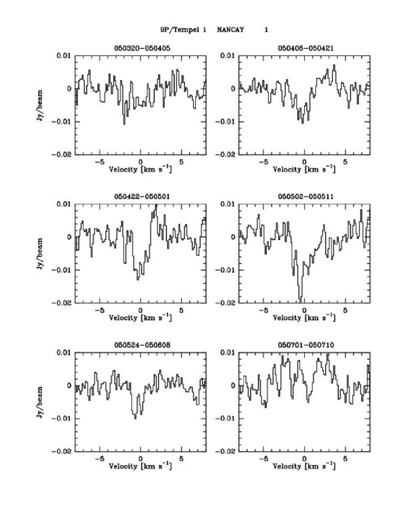
Figure 1: Selected spectra of the OH radical observed in comet 9P/Tempel 1 with the Nançay radio telescope.

The Nançay radio telescope is a meridian telescope with a fixed primary spherical mirror (35 $\times$ 300 m), a secondary plane mirror (40 $\times$ 200 m) tiltable on an horizontal axis and a focal system that can track the source during approximately one hour around time of transit. For the observations of comet 9P/Tempel 1, transiting at $51\mbox{${}^{\circ}$}$ to $32\mbox{${}^{\circ}$}$ elevation, the beam size at 18-cm wavelength is 3.5$\times$19’. Both polarizations of the two hyperfine transitions of the OH $\Lambda$-doublet at 1665 and 1667 MHz were observed every day in the comet from 4 March to 8 June and from 1 to 10 July 2005. The comet was too weak to be detected on a single day of observation but was detected on averages of about 10 days since 20 March (Crovisier et al. 2005). The observations are listed in Table 1 and examples of the observed spectra are shown in Fig. 1.

Observations were reduced and production rates calculated as has been regularly done for previous observations (Crovisier et al. 2002), assuming isotropic outgassing and taking into account collisional quenching of the maser (Table 4). The UV pumping by the solar radiation field is responsible for the population inversion $i$ of the ground state $\Lambda$-doublet of OH that makes the comet emission detectable (Despois et al. 1981; Schleicher & A’Hearn 1988). The Swings effect makes $i$ very sensitive to the heliocentric velocity of the comet. In July $i$ was close to zero (+0.03 or +0.08 on average, depending upon the inversion model). This partly explains why the comet was not detected at Nançay at that time. The Nançay upper limit is consistent with the water production rates observed by other means (see below) and with the OH signal detected with the Green Bank Telescope (Howell et al. 2005).

[Table 1]

[Fig. 1]

2.2 IRAM 30-m telescope

Comet 9P/Tempel 1 was first observed between 4.8 and 9.0 May 2005 with the IRAM 30-m radio telescope, around the time of its perigee. The weather was relatively good and stable, with higher sky opacity on the first night. On the last scheduled night (9.8–10.0 May) observations had to be stopped due to strong winds. In July, the comet was observed every evening from 2.7 to 10.8 July 2005: 6 to 8 hours of observations were scheduled per day, but in general the stability of the atmosphere was relatively poor during the first 3 hours, leading to a typical pointing uncertainty of 5–6” . Later in the evening pointing stability and atmospheric transmission usually improved. The best observing conditions were on 2 and 4 July evenings, while the weather on 6, 8, 9 and 10 July was relatively poor (7 to 12mm of precipitable water versus 2 to 5mm). Every night in May and July, Jupiter and the carbon star IRC+10216 were observed for calibration purpose. The beam sizes and main beam efficiencies ($\eta_{b}\approx 0.76$ to 0.40 depending on frequency) were checked on planets (Jupiter, Saturn or Venus). The calibration of the line intensity and pointing stability were evaluated from observation of the compact source IRC+10216. In addition, other pointing sources within 10–15^∘  of the comet were observed at least every hour.

The observations of the HCN $J$(3–2) line in IRC+10216 were especially useful to estimate the effect of atmospheric instability on the comet line intensity. Anomalous refraction (Altenhoff et al. 1987), which causes random pointing offsets, was the main cause of signal losses in July. Indeed, at this frequency the antenna half power beam width is 9.4”which makes observations very sensitive to pointing. In May, the mean standard deviation of the daily measurements of the intensity of the HCN $J$(3–2) line in both IRC+10216 and the Orion Molecular Cloud calibration sources was less than 7%. But a drop of 50% of the HCN $J$(3–2) line intensity of IRC+10216 was often observed in July at the beginning of the observations, while the losses decreased to less than 20% at the end of each evening shift. The effect on the HCN $J$(1–0) line intensity was much smaller (less than 10% variation) due to the larger beam. These variations could be well attributed to an average pointing offset – as provided in Table 2 – which was larger at the beginning of the observations.

HCN $J$(1–0) and HCN $J$(3–2) lines were detected both in May and July. Average spectra are shown in Figs. 2,5 and 6. Evidence of time variability in the HCN line intensities that could be attributed to the rotation of the nucleus was readily seen in May (Biver et al. 2005). H₂S (Fig. 3) and CH₃OH were also marginally detected in May. Up to three individual lines of CH₃OH lines at 145 GHz were detected in July (Fig. 4). Other species (CS, CO, H₂CO) were searched for both in May and July but not detected. Line intensities or 3-$\sigma$ upper limits are reported in Table 2.

[Fig. 2]

[Fig. 3]

[Figs. 4]

[Figs. 5 and  6]

2.3 CSO telescope

In contrary to IRAM 30-m, the CSO with 10.4-m telescope on top Mauna-Kea, Hawaii, was in direct viewing of comet 9P/Tempel 1 at the time of the encounter with Deep Impact. Although benefiting from a better sky transparency (average amount of precipitable water was 1–2 mm versus 3–4 mm at IRAM on 4–5 July), this 10.4-m radio telescope has a lower sensitivity than the IRAM 30-m and could only observe during 4 h between sunset and comet set. Observations were targeted on the day of the impact and the next one. The 345 GHz double-sideband receiver was used and tuned to the pair of methanol lines at 304.2 and 307.2 GHz, predicted to be among the strongest lines in this wavelength domain (e.g. Biver et al. 2000). In addition, they can provide precise information on the gas temperature. Observations started at 5 h UT on 4 July until 9 h UT and from 1.5 to 8 h UT on 5 July 2005 with tuning to the HCN $J$(4–3) line at 354.5 GHz after 6 UT. Jupiter was used as a pointing and beam efficiency calibration source ($\eta_{b}\approx 0.6$ at 305 GHz and 353 GHz).

A marginal detection of the CH₃OH lines at 304/307 GHz (4-$\sigma$, Fig 7) was obtained on the 4.3 July post-impact data after the two lines (expected to have similar intensities) were co-added. HCN was not detected. Line intensity and upper limits are given in Table 2.

[Figs. 7]

2.4 Odin satellite

The Odin satellite (Nordh et al. 2003, Frisk et al. 2003) houses a 1.1-m telescope equipped with 5 receivers at 119 GHz and covering the 486–504 GHz and 541–580 GHz domains that are in large part unobservable from the ground. Half of the time is dedicated to astronomical studies and the other half to aeronomical investigations. Comets are a major topic for Odin observations and the fundamental rotational line of water at 556.936 GHz has been detected in 11 comets between 2001 and 2005. In addition H${}_{2}^{18}$O at 547.476 GHz and NH₃ at 572.498 GHz were detected in some comets (Biver et al. 2006b).

Comet 9P/Tempel 1 was observed during the “eclipse period”, when part of Odin orbit lies in the Earth shadow, so that only one receiver at 557 GHz could be used due to power limitations. The single-side band receiver system temperature ($Tsys$), which is measured three times per orbit, was $3100\pm 30$ K in June, $3200\pm 60$ K in early July and about 3350 K at the end of July and beginning of August. Variations of $Tsys$ with time were smooth and the resulting calibration uncertainty was below 1%. Two spectrometers were used: the wide band Acousto-Optical Spectrometer (AOS) (1 GHz with 0.6 MHz channel spacing and 1 MHz resolution) and the high resolution AC2 autocorrelator (112 MHz bandwidth, 125 kHz channels, 333 kHz resolution after Hanning smoothing; Olberg et al. 2003). The high resolution corresponds to 180 m s^-1 at 557 GHz, well enough to resolve the $\approx$1.5 km s^-1  wide cometary line. 95 orbital revolutions of 1.6 h, in series of 4–5 consecutive “orbits”, were allocated to the 9P/Tempel 1 program. Due to orbital constraints the comet was observed only 45 to 55 min per revolution. The observations during the ten “orbits” scheduled on 7/8 June mostly failed due to an error in the setup of the spectrometers while three “orbits” on the 17 June and two on the 3rd of July were pointed too far from the target. A 2$\times$2’ map was obtained on 18 June, while on other dates the observations were aimed at the comet nucleus position. The residual pointing offset (checked on Jupiter maps) and uncertainty are estimated to be less than 20”. The beam size at 557 GHz is 127” and main-beam efficiency $\eta_{b}=0.85$. Due to the weakness of the comet, the signal was averaged over 4 to 6 “orbits”. This offers a time resolution (6–10 h) and sensitivity to the amount of gas released by the impact which are better than what the submillimeter wave satellite (SWAS) could achieve (Bensch et al. 2006). Due to standing waves and other interferences, several ripples were present in the spectra and removed with sinusoidal baseline fitting. The line intensities and velocity shifts given in Table 2 are the average of AC2 and AOS values.

[Table 2]

3 Data analysis

3.1 Molecular production rates

Intensities of millimetre and submillimetre lines were converted into production rates using the same modelling and codes as in previous papers (e.g. Biver et al. 1999, 2000, 2002, 2006a, 2006b). A Haser model with symmetric outgassing – unless specified (Section 4.2) – and constant radial expansion velocity are used to describe the density, as in our previous studies. The variation of the photo-dissociation lifetimes of H₂O and HCN due to solar activity is taken into account.

The expansion velocity ($v_{exp}$) is estimated from the line shapes of the spectra with highest signal-to-noise ratios. For May observations we use $v_{exp}=0.65$ km s^-1  (half widths at half maximum intensity, $HWHM=0.70\pm 0.05$ and $0.67\pm 0.13$ km s^-1 for the HCN $J$(3–2) blue and red-shifted sides). In June–July there is more scatter in the measurements: $HWHM=0.78$ and $0.69\pm 0.05$ km s^-1  for H₂O, $HWHM=1.00$ and $0.58\pm 0.15$ km s^-1  for HCN $J$(3–2) and $HWHM=0.75$ and $0.41\pm 0.11$ km s^-1  for HCN $J$(1–0), for blue and red-shifted sides of the lines, respectively, and we adopted an average value of $v_{exp}=0.75$ km s^-1. We used 0.65 km s^-1  for H₂O data obtained after mid-July when lines were narrower ($HWHM=0.77$ and $0.42\pm 0.07$ km s^-1  for H₂O). The variation of the line shape and expansion velocity will be discussed in Sections 4.2 and 4.3.

Our model of excitation of the rotational levels of the molecules takes into account collisions with neutrals at a constant gas temperature. Collisions with electrons also play a major role and are modelled according to Biver (1997) and Biver et al. (1999) with an electron density multiplying factor $x_{ne}$ set to 0.3 for all data. The electron density obtained with a factor $x_{ne}=0.2$–0.3 was found to provide the best match to the radial evolution of line intensities observed for several comets in extended Odin H₂O maps (Biver et al. 2006b). Interpretation of millimetre data (Biver et al. 2006a) usually requires a slightly higher factor, around 0.5. Data obtained in 9P/Tempel 1 cannot put stringent constraints on this free parameter, but the coarse map of H₂O($1_{10}-1_{01}$) obtained in June is as well matched with intensities computed with $x_{ne}$ from 0.1 to 1.0. We adopted the mean value of $x_{ne}=0.3$: using $x_{ne}=0.2$ would increase systematically all H₂O production rates by 7% and using $x_{ne}=0.5$ would decrease them by 10%. The optical thickness of the water rotational lines is taken into account into the excitation process using the Sobolev “escape probability” method (Bockelée-Morvan 1987). We have weak constraints on the gas temperature: in May, from simultaneous observations of the two HCN $J$(3–2) and $J$(1–0) lines, we infer a rotational temperature of $12.2\pm 1.1$ K. Given the assumed collision rate, this corresponds to kinetic temperature of $14^{+11}_{-8}$K. For July data we do not expect a much higher temperature (given that the generally observed trend in previous comets is $T\propto r_{h}^{-1}$ to $r_{h}^{-1.5}$) and assume $T=20$ K. This is slightly lower than the kinetic temperature estimated from infrared spectroscopy by Mumma et al. (2005) but this discrepancy has always been observed when comparing radio and infrared measurements, which are made with different instrumental fields of view. A temperature of only 18 K was measured in the more active comet C/1996 B2 (Hyakutake) at $r_{h}=1.55$ AU (Biver et al. 1999).

A radiative transfer code, taking into account line optical thickness, is used to compute line intensities and to simulate line profiles. The mean opacity of the 557 GHz water line is $<$ 1 and its line intensity is almost proportional to the water production rate for values in the range 5–12$\times 10^{27}$ molec. s^-1 . Other lines considered in this paper are optically thin.

3.2 Simulations of time-variable outgassing rates

A caveat of radio observations is their large field of view, which samples molecules released by the nucleus at different times. The smaller the beam, the more likely the signal will reflect the outgassing behavior of the nucleus in real time. Since we cannot retrieve time dependent information on the true nucleus outgassing rate directly or in a simple way, the best is to try to simulate the observations with a minimum number of free parameters. For all observations and simulations, unless specified, line intensities are converted into “apparent” production rates, i.e., the production rates which would give the observed line intensities assuming a stationary regime. Apparent production rates are computed following the description given in Sect. 3.1.

3.2.1 Simulation of periodic fluctuations

First, we investigate the effect of a periodic fluctuation in outgassing rate in order to interpret the periodicities observed in HCN line intensities in May and, more marginally, in H₂O measurements obtained in July (Sect. 4), both related to nucleus rotation. We assumed an outgassing rate with a sinusoidal periodicity of 1.7 days and an amplitude of 50% of the mean value. This periodic variation is accounted for when computing collisional excitation and radiation transfer. Isotropic outgassing, constant velocity and temperature are otherwise assumed. The expected line intensities for May and July observing conditions were computed for various phases. They were then converted into apparent production rates for direct comparison to the input true production rate. The result is a quasi sinusoidal variation of the apparent production rate which amplitude and phase are retrieved from the fit of a sinusoid. This provides us with information on the extent to which the amplitude of variation is reduced due to beam averaging, and the periodic variation is shifted in phase (the phase shift is hereafter called “beam delay”). As test cases, we studied the HCN $J$(1–0) and HCN $J$(3–2) lines observed at IRAM (which encompass the whole range of CSO and IRAM beam sizes (9.5–27”)) and H₂O observed with Odin.

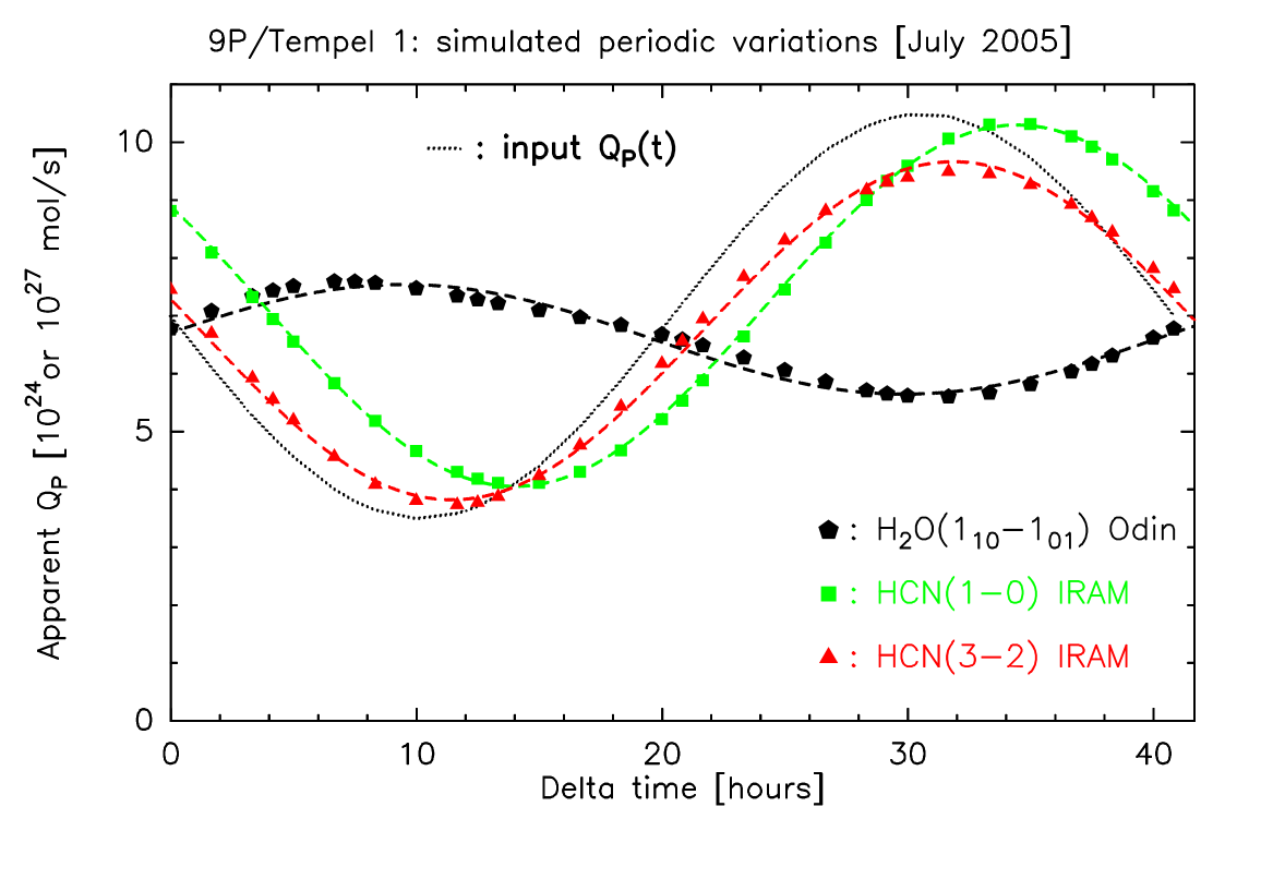
Figure 8: Simulation of the effect of a sinusoidal variation of the HCN and H₂O production rates (dotted line) on apparent production rates measured on different lines with Odin or IRAM for the July observing conditions. Dashed lines are the least squares sinusoidal fits to the computed values. This plot shows the phase shifts (“beam delay”) and amplitude attenuations due to the corresponding beam sizes of the instruments. The simulation for HCN observations in May yields very similar results.

Figure 8 shows the model line intensities converted into “apparent” production rates. The periodicity expected in signals observed at IRAM is delayed by 1.1 h (HCN $J$(3–2)) to 3.6 h (HCN $J$(1–0)), and the delay for H₂O observed by Odin in July is 19.7 h. The amplitude is reduced by 14% (HCN) to 70% (H₂O). Since observations are averaged over a few hours, the amplitude of variation is further reduced by a factor $\sin(x)/x$ with $x=2\pi t_{o}/T_{p}$, where $T_{p}=1.7$ days and $t_{o}$ is the observation duration (typically 0.2 day for HCN to 0.36 day for H₂O; Table 2). This effect is small for IRAM observations (amplitude typically reduced by 9%) but significant for Odin observations (27%). Overall, the amplitude of variation of apparent H₂O production rates measured by Odin can be expected to be 3.5 times smaller than the amplitude of variation of HCN apparent production rates, if H₂O and HCN productions presented similar periodic fluctuations at the nucleus surface.

For OH at Nançay, intensity variations related to nucleus rotation cannot be detected given the large beam size and the low signal-to-noise ratios obtained daily.

[Fig. 8]

3.2.2 Simulations of outgassing bursts

We investigate here the lines intensity response to an outburst. This study is focussed on the lines actually observed with radio facilities in July 2005 and “H₂O($1_{10}-1_{01}$)” refers to this line seen with Odin beam and “HCN $J$(3–2)” and “HCN $J$(1–0)” refer hereafter to those lines as observed with IRAM beams (9.4”and 26.9”respectively). The outburst is described by a sudden increase $\Delta Q$ of outgassing which then decreases following a half Gaussian with a characteristic time of half decay $\Delta t$. For the test cases, we assumed a total release of material during the outburst $N_{t}$ on the order of $1.3\times 10^{32}$ molecules. The background production rate of water used is $Q_{m\rm H_{2}O}=8\times 10^{27}$ molec. s^-1 .

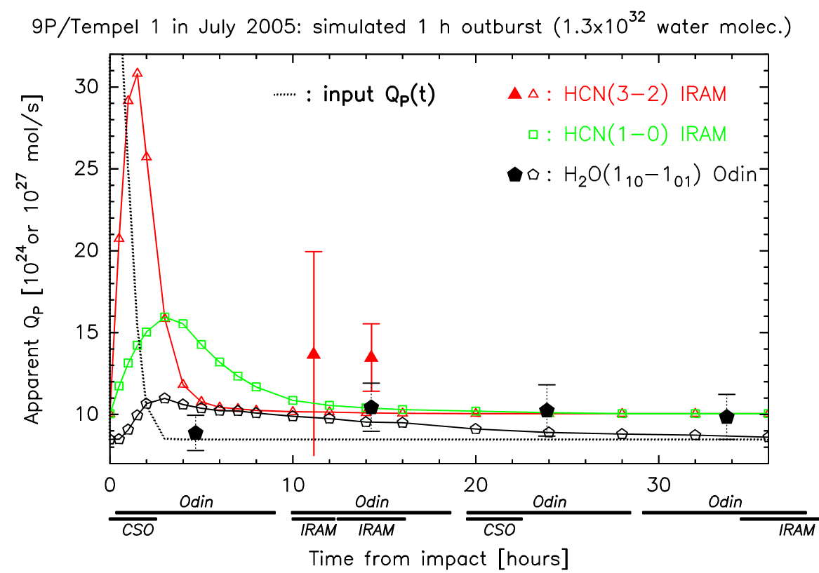
Figure 9: Simulation of the effect of an outburst of $1.3\times 10^{32}$ water molecules ($0.12\times 1.3\times 10^{30}$ for HCN) released isotropically in 1 h, at a velocity of 0.75 km s^-1(dotted line). Connected open symbols are the apparent simulated production rates, as in Fig. 8. The observing time intervals of Odin, IRAM and CSO after 4.244 July are depicted below the bottom axis with horizontal bars. Measurements ($8\times 10^{27}$ molec. s^-1 + excess of outgassing given in Table 7 for water) are plotted with filled symbols and error-bars.

Two kinds of outbursts were considered. In the first case, we assumed that the outburst results in an isotropic distribution of the material. Released HCN and CH₃OH molecules during the outburst are in 0.12% and 2.7% relative proportion with respect to water, respectively. We investigated the cases $\Delta t=1$ h (i.e., $\Delta Q/Q=4.24$) and $\Delta t=15$ h ($\Delta Q/Q=0.28$). The temperature and expansion velocity of the gas are supposed to remain constant with time and throughout the coma. For illustration purposes, the cases ($\Delta t=1$ and 15 h) for HCN and H₂O are shown in Fig. 9 and 10.

[Fig. 9 and 10]

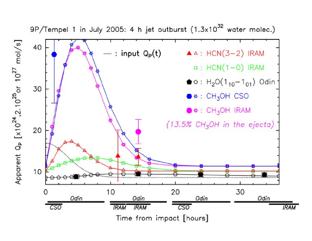
Figure 11: Simulation of the effect of an outburst of $1.3\times 10^{32}$ water molecules released in 4 h (dotted line). The release is limited to a jet in the plane of the sky with a $\pi/2$ steradians opening angle and a velocity of 0.35 km s^-1. The HCN abundance relative to water is 0.12%. For CH₃OH, the abundance relative to water inside the jet is 13.5%, versus 2.7% in the surrounding coma, as suggested by the observations. Measurements ($8\times 10^{27}$ molec. s^-1 + outgassing in a jet from Table 7 for water; mean value plus excess found for the other molecules) are plotted with filled symbols and error-bars.

In another simulation the outburst is restricted to a cone of $\pi/2$ steradians in the plane of the sky with molecules outflowing at a lower velocity ($v_{exp}=0.35$ km s^-1). This more extreme case will provide a better simulation of the observed H₂O line shapes (Section 5.1), and is more realistic since the centre of the cone of ejecta produced by the impact was indeed close to the plane of the sky (A’Hearn et al. 2005b). We also assume that the abundance of CH₃OH relative to water is 13.5%, i.e., 5 times the value in the surrounding coma for direct comparison with the observations (Sect. 5.2). The simulations for $\Delta t=4$ h and 10 h are shown in Figs. 11 and 12.

[Figs. 11 and 12]

[Table 3]

Table 3 summarizes the characteristics of the simulated bursts that would be observed for H₂O with the Odin beam and HCN $J$(3–2) with the IRAM 30-m beam. In summary, the following results are found:

1. Isotropic burst with $\Delta t$ = 1 h: the outburst is seen with a delay of 3–13 h for H₂O($1_{10}-1_{01}$), 1.5 h for HCN $J$(3–2) and about 4 h for HCN $J$(1–0);

2. Isotropic burst with $\Delta t$ = 15 h: the outburst is seen with a delay of $\approx$14 h for H₂O($1_{10}-1_{01}$), $\approx 3$ h for HCN $J$(3–2) and about 7 h for HCN $J$(1–0);

3. $\Delta t$ = 1 to 10 h in a jet of $\pi/2$ steradians in the plane of the sky ($Q_{\rm H_{2}O}=10^{27}$ molec. s^-1 in this cone before burst): the outburst is seen with a delay of about 1 day for H₂O($1_{10}-1_{01}$) and 3–4 h on average for HCN $J$(3–2). The maximum is also significantly attenuated for the H₂O line for the short duration burst due to opacity (at the beginning the local density is multiplied by 56 if $\Delta t=1$ h), (Figs. 11 and 12);

Because the time delay is 0.5 to 1 day for H₂O with Odin, continuous observations over nearly two days after the impact (as performed) are needed to possibly detect impact-related water excesses. On the other hand, a few (3–7) hours after the end of the outburst, we do not expect significant impact-related signal excesses in IRAM and CSO observations. A more continuous worldwide coverage would have been useful.

The simulations also show that, under the assumption of an isotropic outburst, the total number of molecules injected in the burst can be retrieved by integrating over time the apparent production rates. This is indeed expected for optically thin lines. There are only limited photon losses for H₂O (10% for the 1 h burst, much less for the 15 h duration burst) due to moderate opacity effects. Losses become important for water when considering a cone-restricted outburst, because of high local densities: 64, 32 and 18 % for 1, 4, 10 h bursts, respectively, for the geometry considered here.

4 Intrinsic variations of the outgassing and molecular abundances

Table 4 lists “apparent” production rates computed according to Section 3.1. In this section, we will present long-term trends and periodic variations observed in the data, a necessary step to determine relative molecular abundances and study the increase of molecular production due to the impact excavation.

[Table 4]

4.1 Long-term evolution of the outgassing

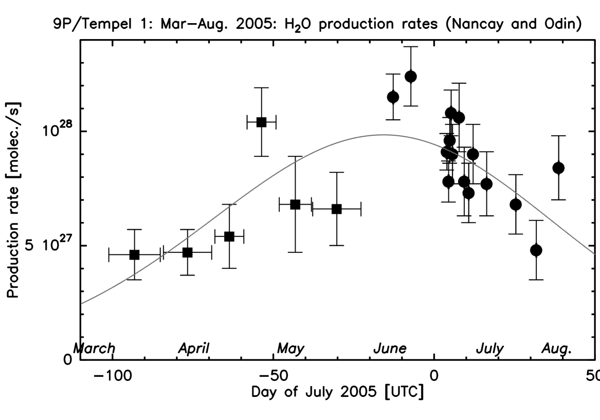
Figure 13: Water production rates based either on Nançay observations of the OH radical (squares) or Odin observations of the H₂O line at 557 GHz (circles). The continuous curve corresponds to Eq. (1) deduced from the least squares fitting.

Fig. 13 shows the evolution of the water production rate from March to August 2005. The least squares fitting of a Gaussian to the water production rates, taking into account a $r_{h}^{-2}$ heliocentric evolution due to increased solar irradiance as the comet gets close to the Sun, yields:

$$Q_{\rm H_{2}O}=10.0\times 10^{27}\exp\left(-\left(\frac{t+23}{88}\right)^{2}\right)\times\left(\frac{1.506}{r_{h}}\right)^{2},$$ (1)

where $t=$date$-T_{perihelion}$ in days. The 23 June data point is not included in this analysis (cf. Section 6). The fit is marginally significant ($\chi^{2}=27$ versus 41 for no variation), and might be biased by the inhomogeneity of the data (Nançay versus Odin). Indeed, H₂O production rates derived from Nançay and Odin simultaneous measurements show sometimes significant discrepancies (Colom et al. 2004). A peak of activity before perihelion is suggested. This is in agreement with previous perihelion passages, though the peak in production was near 2 months before perihelion rather than 3 weeks (see the review of Lisse et al. 2005). This pre/post perihelion asymmetry could be due to the presence of an active region close to the nucleus south pole which is no longer illuminated after May–June (a fan-shaped structure was indeed observed to the south of the comet in March–May optical images). This also suggests a mean production rate around the time of the impact of $9.3\times 10^{27}$ molec. s^-1 , in agreement with other measurements: $6\times 10^{27}$ (Schleicher et al. 2006), $7\times 10^{27}$ (Bensch et al. 2006) to $10\times 10^{27}$ molec. s^-1 (Mumma et al. 2005).

[Fig. 13]

4.2 Periodic variations of the HCN production rate

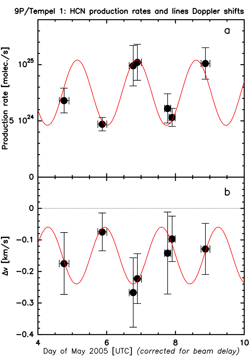
Figure 14: Top: HCN production rates based on IRAM 30-m observations in May 2005, based on isotropic outgassing. A sinusoidal fit to the data is plotted (Eq. (2)). Bottom: Doppler shifts of the HCN$J$(1–0) and HCN$J$(3–2) lines observed at IRAM 30-m in May 2005. The sinusoidal fit to the data (Eq. (3)) is plotted. All times were corrected for “beam delay” (cf. text).

Fig. 14a shows the HCN “apparent” production rate versus time observed in May. Data were split into two time intervals per night and the production rates based on HCN(1–0) and HCN(3–2) plotted separately (although the temperature is one fixed parameter that makes them not fully independent). Day-to-day variations with some periodicity are observed, as for the line intensities (Table 2).

We first searched for periodicity with the phase dispersion minimization (PDM) method (Stellingwerf 1978). This method is powerful in unveiling periodicities in a signal, especially when data are irregularly sampled and scarce (Colom and Gérard 1988). The result of the PDM method applied to the 14 data points shows a significant minimum of the variance ratio (around 0.23 which means a significance level of 99%) around 2 days with deeper peaks at 1.8 and 2.3 days. The two periods are the result of an aliasing ($1/T_{p}^{\prime}=1/T_{s}-1/T_{p}$ where $T_{s}\approx 1$ day is the the sampling period). The most significant peak is close to the $\approx 1.7$ day estimated rotation period of the nucleus (Belton et al. 2005, A’Hearn et al. 2005b).

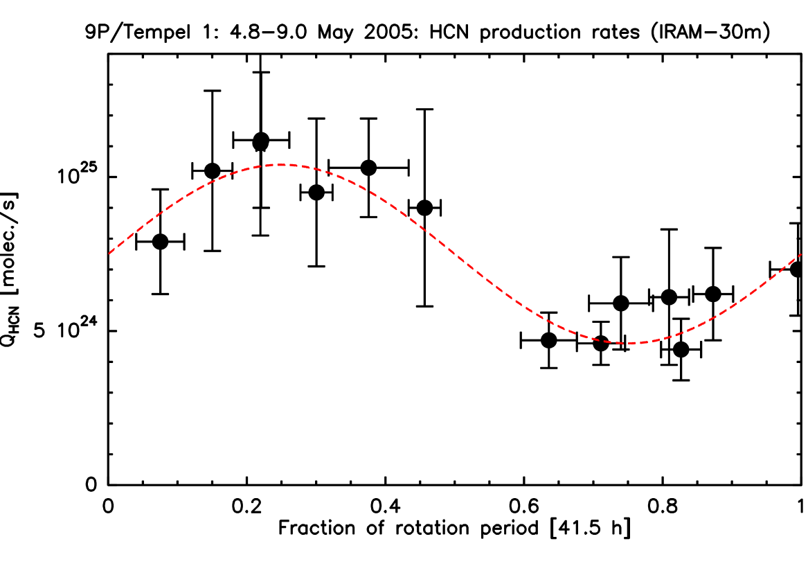
Figure 15: HCN production rates based on IRAM 30-m observations in May 2005 folded on the 1.73 rotation period (Fig. 14, Eq. (2). All the data points (2 per day per line) used in the sine adjustment are shown here. All times were corrected for “beam delay” (cf. text).

The second method was direct fitting of a sine curve to the data. A sine evolution was assumed since the signal-to-noise ratio is not high enough to determine the shape of a periodic variation. Indeed, folding all the 14 points (or 7 points if we average daily measurements as in Fig. 14 to increase the signal-to-noise) over one period cannot discriminate the variation of $Q_{\rm HCN}$ from a simple sine evolution (Fig. 15). A 4-parameter (period $T_{p}$, phase origin $T_{0}$, mean production rate $Q_{m\rm HCN}$ and amplitude $\Delta~{}Q_{\rm HCN}$) weighted least squares fitting over 14 points yields:

• $T_{p}=1.68$ days;

• $T_{0}=6.51$ May 2005;

• $Q_{m\rm HCN}=7.3\times 10^{24}$ molec. s^-1 ;

• $\Delta~{}Q_{\rm HCN}=3.0\times 10^{24}$ molec. s^-1 ;

• $\chi^{2}=3.8$ and the reduced chi-square is $\chi^{2}_{\nu=10}=0.38$.

After “beam delay” correction, we get (Sect. 3.2.1):

• $T_{p}=1.73\pm 0.10$ days;

• $T_{0}=6.44\pm 0.07$ May 2005;

• $Q_{m\rm HCN}=7.5\pm 0.5\times 10^{24}$ molec. s^-1 ;

• $\Delta~{}Q_{\rm HCN}=2.9\pm 0.7\times 10^{24}$ molec. s^-1 ;

• $\chi^{2}=3.1$ and the reduced chi-square is $\chi^{2}_{\nu=10}=0.31$.

which gives:

$$Q_{\rm HCN}=\left(7.5+2.9\times\sin\left[2\pi\frac{t-6.44{\rm~{}May~{}2005}}{1.73}\right]\right)\times 10^{24}\mbox{molec.~{}s${}^{-1}$~{}}.$$ (2)

This curve is plotted in Fig. 14a. The uncertainty on the fitted parameters is obtained by the projection of the 4-D ellipsoid $\Delta\chi^{2}=1$ on the four parameters axes.

[Fig. 14]

[Fig. 15]

The period of HCN variation is very close to the actual rotation period of the nucleus (1.701 days, A’Hearn et al. 2005b). A HCN production curve with two peaks per period, as observed for the nucleus lightcurve, seems excluded from our data. This suggests that one side of the nucleus might have been more productive than the other when illuminated by the Sun. Jehin et al. (2006) found a periodic variation of 1.709 days in the CN and NH fluxes measured in June and around the impact date. Two major peaks were observed in one rotational phase, which were interpreted by the presence of two active regions, the strongest one corresponding to a peak of outgassing taking place on July 4.32 UT equivalent date. A search for periodicity in the July HCN data, for direct comparison with CN data, is not possible given their poorer quality and low signal-to-noise ratios. If the strongest peak seen in CN by Jehin et al. (2006), assuming CN mainly comes from the photodissociation of HCN, corresponds to the maxima observed for HCN in May, then the observations are compatible with a “Tempel day” of 1.719 days (34 rotations between May 6.88 and July 4.32) or $T_{p}=1.715$ days for the sideral rotation period.

The strong variation in HCN production (a factor of $\approx$3) during nucleus rotation shows that “natural” variability of the comet activity must be taken into account when searching for impact-related production excesses.

4.3 Variation of line shapes

Periodic variations are also present in the HCN line shapes observed in May. Fig. 14b shows the evolution of the Doppler shift derived from daily averaged data (Table 2). The least squares sinusoidal fit adjustment yields :

$$\Delta~{}v=-0.15+0.09\sin\left[2\pi\frac{t-7.18{\rm~{}May~{}2005}}{1.65}\right]~{}\mbox{km~{}s${}^{-1}$},$$ (3)

with the date $t$ in days corrected for “beam delay”. The period of variation $T_{p}=1.65^{+0.31}_{-0.14}$ days is in agreement with previous findings. The reduced $\chi^{2}$ is $\chi^{2}_{4}=0.13$, versus $\chi^{2}_{6}=0.69$ for a straight line fit to the 7 data points with mean Doppler shift $\Delta v=-0.14$ km s^-1.

There is a correlation between line shapes and line intensities (Table 2, Fig. 2). The blueshift of the lines is at its maximum at the time of maximum outgassing. This can be explained by an active source which molecular production varies with solar illumination when the nucleus is rotating. A simple simulation with a broad ($\pi/2$ steradians) rotating HCN jet actually provides a good match to the observed line strengths and shapes.

4.4 Short-term variation of the water production rate

The evidence of periodic variation in outgassing seen in HCN May data or for several gaseous species in June–July (Jehin et al. 2006) convinced us to look for variation in H₂O production rates measured with Odin. But as explained in Sect. 3.2.1, we expect the amplitude of the variation of the H₂O($1_{10}-1_{01}$) line observed by Odin to be 3.5 times lower than that for HCN observed at IRAM. In Fig. 16 we have plotted the average $Q_{\rm H_{2}O}$ corrected for $1/r_{h}^{2}$ heliocentric evolution and excluding the July 4.4–7.8 post-impact data. The mean value is $Q_{m\rm H_{2}O}=8.0\times 10^{27}$ molec. s^-1 at perihelion, so that the apparent amplitude of periodic variation similar to those seen for HCN would be on the order of $0.9\times 10^{27}$ molec. s^-1 , similar to each individual measurement uncertainty.

Actually fitting a sine evolution with fixed phase ($T_{0}=3.90$ July + 0.82 day (cf. Sect. 4.2 and “Beam delay”) and period (1.71 days), yields:

$$Q_{\rm H_{2}O}=\left(8.1+0.7\times\sin\left[2\pi\frac{t-4.72}{1.71}\right]\right)\times\left(\frac{1.506}{r_{h}}\right)^{2}\times 10^{27}\mbox{molec.~{}s${}^{-1}$~{}}.$$ (4)

The reduced chi-square is $\chi^{2}_{6}=1.32$, to be compared to $\chi^{2}_{5}=1.29$ when fitting just the mean value $Q_{m\rm H_{2}O}\times(1.506/r_{h})^{2}$. Periodic variations cannot be reliably retrieved from Odin data, but the attempt to fit a sine variation to the data shows that a strong variation of outgassing with rotation phase of the nucleus is not excluded: the fitted amplitude is similar to the expected one (Sect. 3.2.1), about 1/3${\rm rd}$ of the amplitude of the CN variations seen by Jehin et al. (2006) to 1/4${}^{\rm th}ofQ$HCN variations in May. So, a variation in natural outgassing should be taken into account when looking for impact related effects. Indeed, as shown by Jehin et al. (2006), $T_{0}\approx 3.90$ July means that “natural” outgassing of the nucleus was in its rising phase at the impact time (4.244 July), peaking 3–4 h later.

[Fig. 16]

For the purpose of determining molecular abundances based on IRAM observations in May, we will use a reference water production rate:

$$Q_{\rm H_{2}O,ref}=\left(8+3\sin\left[2\pi\frac{t-0.1-({\rm 6.44~{}May~{}2005})}{1.72}\right]\right)\times\left(\frac{1.506}{r_{h}}\right)^{2}\times 10^{27}\mbox{molec.~{}s${}^{-1}$~{}}.$$ (5)

It matches the May periodicity of HCN and the April-May mean water production rate derived from Nançay observations ($7\pm 1\times 10^{27}$ molec. s^-1 ). $t$ is the number of days since 0.0 May 2005 UT with a 0.1 day shift added to take into account the “beam delay” for millimetre observations. The computed reference water production rates are given in column 5 of Table 4.

4.5 Mean molecular abundances

Molecular production rates were ratioed to the reference water production rate in order to derive the molecular abundances given in Table 5. The abundances did not vary significantly between May and July and the mean values (H₂O:CO:CH₃OH:H₂CO:H₂S:HCN:CS) = (100 : $<10$ : 2.7 : $<$1.5 : 0.5 : 0.12 : $<$0.13) fall well within the typical abundances measured in about 30 comets since 1986 (Biver et al. 2002, 2006a).

5 Amount of gas released by the impact

Cautiously taking into account intrinsic periodic variations of the outgassing rate, we can now estimate the contributions from the impact or outburst related activity. However, one problem is that the excess of signal will not only depend on the number of molecules released but also on their velocity and the duration of the burst in outgassing. The simplified simulations presented in Sect. 3.2 will guide our analysis.

5.1 Water

For H₂O data, the simplest way (model (1)) to evaluate the outgassing excess due to the impact is to compute the difference between the observed apparent production rates (Table 6, column 4) and a reference production rate. The reference production rates are taken from the last column of Table 6. The right part of this table provides lines characteristics and apparent production rates based on Odin observations between 7 July and 7 August binned according to the expected rotation phase (Column 1). Using the sine function of Eq. 4 would give very similar results.

[Table 6]

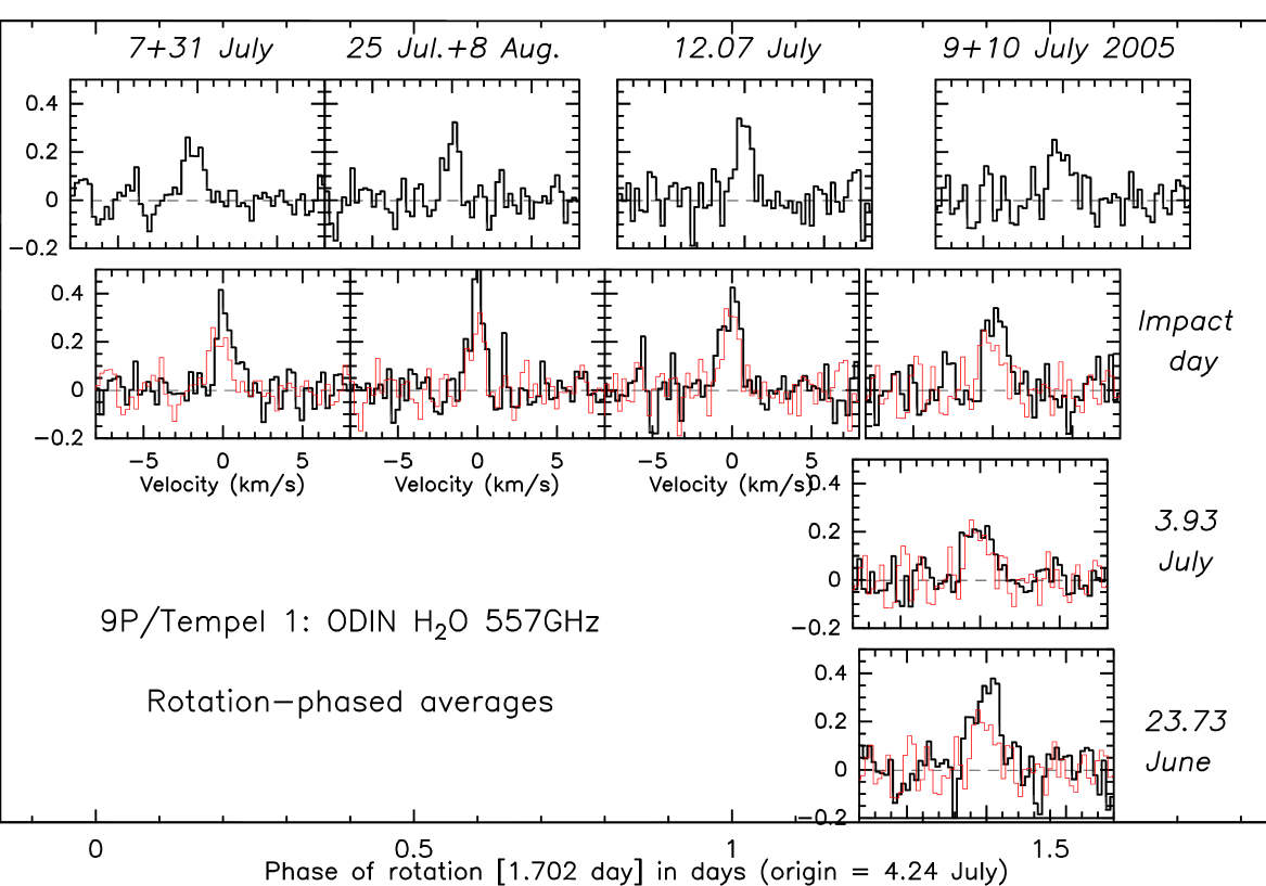
Figure 17: Spectra of H₂O obtained with Odin summed and ordered according to the phase of the comet rotation (1.7 day, horizontal scale) and time (vertical scale, from before the impact (bottom) to after the impact (top row)).

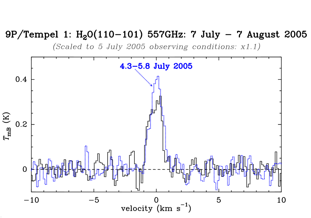
Figure 18: The 557 GHz H₂O line observed by Odin after the Deep Impact collision. Dotted line: an average of observations obtained during the first rotation just following the impact. Solid line: an average of observations obtained between 7.7 July and 7.7 August, after dissipation of the impact ejecta cloud. These observations were sampled and averaged to cover a full nucleus rotation. They were scaled to correct for the decrease of the signal due to the change in geocentric and heliocentric distances.

The main difference between the reference and impact spectra is a narrow spike around zero velocity which is superimposed on a broader component and is only seen on the 4.4–5.6 July high resolution spectra (Figs. 17 and 18). Correcting for the slightly different geometries at different dates, the line integrated intensity of this spike was estimated, as given in Table 7. It is close to the excess signal seen above $T_{mb}=0.25$ K. The conversion of this line intensity into a number of molecules is not straightforward since the H₂O line is optically thick: photons emitted by the cloud of ejecta responsible for this spike will be absorbed by the foreground H₂O coma. This process was not considered. We expect that the results are not affected by a large factor, since both the spike position ($v\approx 0.0$ km s^-1) and geometry of the ejecta suggest that this cloud was in the plane of the sky, minimizing line-of-sight opacity effects. The narrow width of the spike ($HWHM=0.22\pm 0.05$ km s^-1) also suggests a relatively low velocity of $v_{exp}\approx 0.35$ km s^-1, if we assume an opening angle of 90^∘ for the cloud of ejecta. This low velocity also minimizes photon absorption by the higher velocity surrounding gas. For this second estimate of the amount of gas inside the ejecta (model (2)), we run our radiative transfer code with the molecules distributed inside a cone of opening angle of 90^∘, and expanding at $0.35$ km s^-1.

[Figs. 17, 18]

Table 7 provides impact-related apparent production rates as a function of time, and corresponding total amounts of H₂O molecules, for the two different analyses. As discussed in Sect. 3.2, these numbers should be close to the total number of molecules released in the burst.

[Table 7]

Although based on the same data, models (1) and (2) give different results for the apparent production rate (line 5 in Table 7). This is because model (2) assumes a lower velocity in order to interpret the narrow spike. However, similar amounts of molecules are derived from the two models. Indeed, for model (2) we take into account that part of the emitted photons are lost by self-absorption effects, as discussed in Sect. 3.2. The time evolution of the apparent production rates derived from model (2), when compared to the simulations, provides a good agreement with a 4–10 h duration outburst (Figs. 11 and  12) and $N_{t}=1.3-2\times 10^{32}$ molecules. Mumma et al. (2005) found an excess of $10^{28}$ molec. s^-1 in water production in the 1–3 h following the impact, on the basis of infrared measurements inside a $\approx 1$”aperture for which beam dilution and beam delay can be neglected. The sublimation of 5000 tons of water ice at a rate of $\approx 10^{28}$ molec. s^-1 would take $\approx$ 4 h. Therefore, the observations of Mumma et al. (2005) are consistent with the simulation shown in Fig 11.

In summary, the two approaches yield consistent values for the amount of water released by the impact. We adopt a mean value of $5000\pm 2000$ tons ($N_{t}=1.7\times 10^{32}$ molecules), given that the increase of outgassing due to the impact is detected at the 3–4 $\sigma$ level (line 5, column 7 of Table 7 and Fig. 18) and that the uncertainty due to excitation parameters (e.g. electron density) can be on the order of 10% or slightly higher. This amount is also consistent with estimates based on near-UV observations of OH by Küppers et al. (2005) ($\approx 4500$ tons) and Schleicher et al. (2006) ($<13000$ tons).

5.2 Other molecules

Due to limited signal-to-noise ratios ($\approx 5$ for HCN and CH₃OH, versus 10 for H₂O), the millimetre lines do not show clear evidence of emission excesses related to the impact. Most of the observations took place more than 10 h after the impact, which implies that most of the material had already left the beams. From the various simulations discussed in Section 3.2, we can mainly note that the beam delays are on the order of 2 h (HCN $J$(3–2)), 4 h (CH₃OH) to 7 h (HCN $J$(1–0)). Therefore the millimetre molecular observations are much more sensitive to the time it took to the ejected icy grains to sublimate than are Odin H₂O observations.

Figs. 5 and  6 show the spectra of both the HCN $J$(1–0) and HCN $J$(3–2) lines at IRAM on the day of the impact (4.84 July 2005) and the averages before (2.8–3.8 July) and after (5.8 July) the impact. The lines appear to be stronger on 4.84 July (Table 2), which can be partly due to a larger intrinsic outgassing at that time (peak around 4.4 July). From May, 2–3 and 5–10 July data, we derive a mean abundance $Q_{\rm HCN}/Q_{\rm H_{2}O}=0.12\pm 0.03$% (Table 5). The excess observed at $t_{0}$+14 h on 4.84 July is then:

$$\Delta~{}Q_{\rm HCN}=(13.1-0.0012\times 8000)\pm 2.1\times 10^{24}\mbox{molec.~{}s${}^{-1}$~{}}=3.5\pm 2.1\times 10^{24}\mbox{molec.~{}s${}^{-1}$~{}}.$$ (6)

No significant impact-related excess of HCN is thus detected.

The average abundance of methanol relative to water is $2.7\pm 0.3$% (Table 5). Using this value as a reference, the excess of methanol on 4.30 July, just after the impact (assuming a background normal $Q_{\rm H_{2}O}\approx 11\times 10^{27}$ molec. s^-1 , close to its possible peak value at that time) is:

$$\Delta~{}Q_{\rm CH_{3}OH}=5.5\pm 2.4\times 10^{26}\mbox{molec.~{}s${}^{-1}$~{}}~{}~{}(t_{0}+{\rm 1.3~{}h,CSO~{}data)}$$ (7)

and on 4.84 July:

$$\Delta~{}Q_{\rm CH_{3}OH}=1.7\pm 0.6\times 10^{26}\mbox{molec.~{}s${}^{-1}$~{}}~{}~{}(t_{0}+{\rm 14~{}h,IRAM~{}data).}$$ (8)

The methanol excess is still marginal however (2–2.5$\sigma$).

These results are too marginal to derive any secure conclusion. We can only work on the hypothesis that 5000 tons of water were released in probably 4 hours or more. According to Beer et al. (2006), 1–10$\mu$m icy grains would sublimate in 0.5 h to more than 24 h at 1.5 AU, depending on their water ice fraction. Deep Impact observations and XMM-Newton observations (Schulz et al. 2006) actually detected icy grains in the coma of the comet at least during the first hour following the impact.

The excesses of outgassing found for HCN and CH₃OH are plotted in Figs. 11 and 12 which present the evolution of the “apparent” production rate expected from the simulations for H₂O:CH₃OH:HCN ratios of 100:2.7:0.12. The measurements are compatible with a normal abundance of HCN in the ejecta, while an overabundance of CH₃OH is suggested. Indeed, to explain both CSO and IRAM observations with the same total quantity $N_{t\rm CH_{3}OH}$ of methanol released in the ejecta, an outburst lasting around 4 h is required, with $N_{t\rm CH_{3}OH}=46\pm 18\times 10^{30}$ molecules. This implies a relative abundance CH₃OH/H₂O$=27\pm 11$% in the ejecta, i.e., one order of magnitude larger than the abundance measured for normal activity. However, the methanol impact spectra (Figs. 4 and 7) do not show any obvious feature such as the H₂O spike. So, it is not excluded that part of the excess signal (or loss on the other dates) is due to calibration or modelling uncertainties. Indeed Mumma et al. (2005) find that the CH₃OH/H₂O ratio in the ejecta was not significantly different from the background.

Only upper limits have been obtained for molecules observed far from the impact time. An upper limit of $22$% relative to water is measured for CO on the day of the impact. Even assuming that the CO abundance relative to water was 10% (maximum allowed by May observations) before the impact, the remaining 12% yield an upper limit on the CO quantity in the ejecta much larger than that of water. This result does not provide useful constraints.

6 Other outbursts of activity

Several bursts of activity were reported by the cameras of the Deep Impact spacecraft before the encounter (A’Hearn et al. 2005b), or by other observations in visible to X-ray wavelengths (e.g. on 8 July, Meech et al. 2005b). Comparing the observed production rates of water with the expected natural variations, we found significant differences on two dates with $\Delta Q_{\rm H_{2}O}=4.0\pm 1.2\times 10^{27}$ molec. s^-1 on 23.7 June and $\Delta Q_{\rm H_{2}O}=2.9\pm 1.4\times 10^{27}$ molec. s^-1 on 7.7 July (Table 4). The stationary regime assumption is of course not relevant to analyze these outbursts, and the $\Delta Q_{\rm H_{2}O}$ value given above (about +50%) are just indicative.

The July 7.7 outburst does not correspond to a very strong or long outburst. Indeed, given the $\approx$ 0.6 day phase delay with IRAM observations, the Odin H₂O data can be compared to HCN or CH₃OH observations on 6.9 and 7.8 July, but nothing significant is observed on these dates. For a half-day burst (cf. Section 4.1), the $\Delta Q_{\rm H_{2}O}$ given above corresponds to $N_{t}\approx 2\times 10^{32}$ molecules, i.e., 1/3 day of normal activity. We note, however, that this outburst is only detected at a 2-$\sigma$ level.

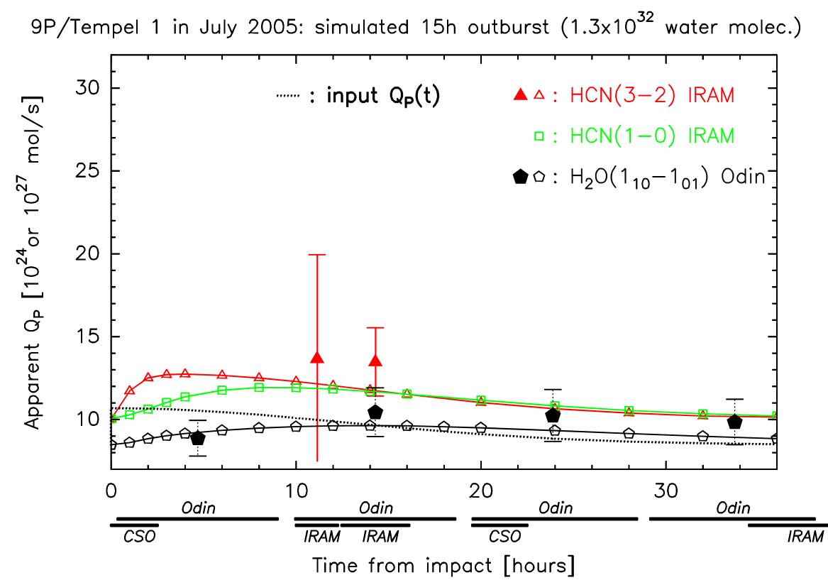
Figure 10: Same as in Fig. 9 but for molecules released in 15 h.

The Deep Impact team reported an outburst beginning on 22.38 June UT. The excess in H₂O emission that we observed 32 hours later is likely related to this outburst. In the spectrum, the extra signal due to this burst of molecules is broader than the impact-related spike (Fig. 17). From a simulation similar to the one shown in Fig. 10, we infer a total release of $N_{t}\approx 10^{33}$ molecules corresponding to 1.4 day of normal activity. This natural outburst surpassed significantly the one created by Deep Impact.

7 Conclusion

Comet 9P/Tempel 1 is certainly one of the weakest comets extensively studied at radio wavelengths, with a peak outgassing rate around $10^{28}$ molec. s^-1 . This investigation campaign puts into evidence several characteristics of the comet:

• The relative molecular abundances are “classical”, of the order of (H₂O:CO:CH₃OH: H₂CO:H₂S:HCN:CS) = (100:$<$10:2.7:$<$1.5:0.5:0.12:$<$0.13), comparable to mean values observed in many comets.

• A strong regular variation of the outgassing rate is clearly observed in HCN data obtained in May 2005 ($T_{p}=1.73\pm 0.10$ days). Its amplitude is a factor of 3 from minimum to maximum and its periodicity is likely related to a rotation period. Outgassing anisotropy is also evident. This suggests that one side of the nucleus was more active than the other when illuminated.

• The periodic variation of the outgassing of the comet must be carefully taken into account when analyzing the effects of the Deep Impact collision. It is not excluded that “natural” outgassing was still varying by $\pm 40$% in early July and that it was in a rising phase at the time of the impact.

• As regards to Deep Impact consequences, the total amount of water released is estimated to $5000\pm 2000$ tons, corresponding to the cumulated production of 0.2 day of normal activity. This water was most likely released in icy grains that took several hours to sublimate: our best guess, based on simulations, is around 4 h. It was not possible to assess precisely the composition of the ejecta, except for a possible increase in the abundance of CH₃OH; no large excess of HCN was seen.

• The comet also underwent significant natural outbursts of outgassing, possibly of larger amplitude than the Deep Impact related burst. One took place on 22–23 June and may have released as much water as 1.4 day of normal activity.

Although the signal was too weak to make a detailed compositional study of the impact ejecta, this observing campaign allowed us to observe in detail the behavior of a Jupiter-family comet, and to put into evidence periodicity and outbursts of outgassing poorly observed in any comet before.

Acknowledgments. Odin is a Swedish-led satellite project funded jointly by the Swedish National Space Board (SNSB), the Canadian Space Agency (CSA), the National Technology Agency of Finland (Tekes) and the Centre National d’Études Spatiales (CNES, France). The Swedish Space Corporation is the prime contractor, also responsible for Odin operations. The authors thanks the whole Odin team, including the engineers who have been very supportive to the difficult comet observations. Their help was essential in solving in near real time problems for such time critical observations. We are grateful to the IRAM and CSO staff and to other observers for their assistance during the observations. IRAM is an international institute co-funded by the Centre national de la recherche scientifique (CNRS), the Max Planck Gesellschaft and the Instituto Geográfico Nacional, Spain. The CSO is supported by National Science Foundation grant AST-0540882. The Nançay radio observatory is the unité scientifique de Nançay of the Observatoire de Paris, associated as Unité de Service et de Recherche (USR) 704 of the CNRS The Nançay observatory also gratefully acknowledges the financial support of the Conseil régional of the Région Centre in France.

Table 1: Observations of OH 18-cm lines in comet 9P/Tempel 1 at Nançay

UT date 2005	$<r_{h}>$	$<\Delta>$	Int. time	$\int T_{b}dv$	Velocity offset	$inversion$
[mm/dd.dd-dd.dd]	[AU]	[AU]	[days$\times$1 h]	[K km s-1]	[km s-1]	(1)	(2)
03/04.11–03/19.06	1.89	0.98	15	$+0.004\pm 0.003$		-0.23	-0.27
03/20.06–04/05.01	1.78	0.82	12	$-0.015\pm 0.003$	$-0.70\pm 0.69$	-0.28	-0.33
04/06.01–04/21.95	1.71	0.75	17	$-0.013\pm 0.002$	$-0.29\pm 0.16$	-0.31	-0.37
04/22.95–05/01.92	1.65	0.72	10	$-0.014\pm 0.003$	$-0.08\pm 0.14$	-0.30	-0.36
05/02.92–05/11.89	1.62	0.71	9	$-0.029\pm 0.004$	$-0.23\pm 0.14$	-0.28	-0.34
05/12.89–05/22.86	1.58	0.72	10	$-0.015\pm 0.004$	$+0.13\pm 0.20$	-0.25	-0.30
05/24.86–06/08.82	1.54	0.76	14	$-0.011\pm 0.002$	$-0.41\pm 0.17$	-0.19	-0.21
07/01.78–07/10.77	1.51	0.90	10	$+0.011\pm 0.004$		+0.03	+0.08

Note: Maser inversion values are from (1) model of Despois et al. (1981) or (2) Schleicher and A’Hearn (1988).

Table 2: Observations of comet 9P/Tempel 1

UT date 2005	$<r_{h}>$	$<\Delta>$	Int. time	Species (transition)	$\int T_{b}dv$	Velocity offset	Offset
[mm/dd.dd-dd.dd]	[AU]	[AU]	[min]		[K km s-1]	[km s-1]
Odin 1.1-m
06/18.06–18.43	1.516	0.818	70	H2O($1_{10}-1_{01}$)	$0.67\pm 0.10$	$-0.31\pm 0.13$	14”
			90	H2O($1_{10}-1_{01}$)	$0.37\pm 0.09$	$-0.08\pm 0.25$	63”
			68	H2O($1_{10}-1_{01}$)	$0.33\pm 0.10$	$+0.38\pm 0.32$	83”
06/23.61–23.85	1.511	0.842	179	H2O($1_{10}-1_{01}$)	$0.66\pm 0.07$	$-0.03\pm 0.11$	14”
07/03.65–04.22	1.506	0.892	375	H2O($1_{10}-1_{01}$)	$0.44\pm 0.04$	$-0.14\pm 0.08$	15”
07/04.26–04.62	1.506	0.895	248	H2O($1_{10}-1_{01}$)	$0.38\pm 0.04$	$+0.15\pm 0.10$	14”
07/04.66–05.02	1.506	0.897	250	H2O($1_{10}-1_{01}$)	$0.46\pm 0.05$	$-0.09\pm 0.10$	14”
07/05.06–05.43	1.506	0.899	250	H2O($1_{10}-1_{01}$)	$0.52\pm 0.05$	$-0.09\pm 0.07$	15”
07/05.46–05.83	1.506	0.901	252	H2O($1_{10}-1_{01}$)	$0.41\pm 0.05$	$+0.17\pm 0.13$	14”
07/07.57–07.84	1.506	0.912	218	H2O($1_{10}-1_{01}$)	$0.50\pm 0.07$	$-0.09\pm 0.13$	12”
07/09.22–09.45	1.507	0.921	165	H2O($1_{10}-1_{01}$)	$0.37\pm 0.07$	$-0.06\pm 0.19$	12”
07/10.57–10.85	1.507	0.929	167	H2O($1_{10}-1_{01}$)	$0.34\pm 0.06$	$-0.11\pm 0.15$	15”
07/11.95–12.19	1.508	0.937	166	H2O($1_{10}-1_{01}$)	$0.42\pm 0.06$	$-0.21\pm 0.16$	12”
07/16.17–16.41	1.510	0.962	206	H2O($1_{10}-1_{01}$)	$0.34\pm 0.06$	$-0.30\pm 0.21$	18”
07/25.21–25.49	1.519	1.020	242	H2O($1_{10}-1_{01}$)	$0.30\pm 0.06$	$+0.15\pm 0.15$	15”
07/31.59–31.87	1.529	1.064	207	H2O($1_{10}-1_{01}$)	$0.19\pm 0.05$	$-0.38\pm 0.22$	20”
08/07.55–07.82	1.543	1.116	201	H2O($1_{10}-1_{01}$)	$0.32\pm 0.05$	$-0.05\pm 0.13$	15”
IRAM 30-m
05/04.76–05.04	1.625	0.711	460	HCN(1–0)	$0.031\pm 0.005$	$-0.18\pm 0.10$	2.0”
05/05.78–06.04	1.622	0.712	418	HCN(3–2)	$0.097\pm 0.012$	$-0.08\pm 0.06$	2.3”
05/06.80–07.04	1.618	0.712	78	HCN(3–2)	$0.213\pm 0.034$	$-0.22\pm 0.08$	2.0”
			178	HCN(1–0)	$0.045\pm 0.008$	$-0.27\pm 0.11$	3.0”
05/07.79–08.04	1.615	0.713	150	HCN(3–2)	$0.112\pm 0.017$	$-0.09\pm 0.07$	2.0”
			200	HCN(1–0)	$0.028\pm 0.006$	$-0.14\pm 0.13$	2.0”
05/08.79–09.04	1.611	0.713	202	HCN(3–2)	$0.212\pm 0.019$	$-0.12\pm 0.08$	2.0”
05/05.78–07.04	1.621	0.712	287	H2S($1_{10}-1_{01}$)	$0.030\pm 0.008$	$-0.28\pm 0.13$	2.1”
05/05.78–09.04	1.615	0.713	818	CH3OH 157 GHz	$0.055\pm 0.008$	$-0.13\pm 0.08$	2.8”
05/04.76–08.04	1.619	0.712	508	CO(2–1)	$<0.025$		2.7”
05/08.79–09.04	1.611	0.713	202	CS(5–4)	$<0.045$		2.5”
05/04.76–05.04	1.625	0.711	230	H2CO($3_{12}-2_{11}$)	$<0.062$		2.0”
07/02.81–03.88	1.506	0.889	221	HCN(1–0)	$0.035\pm 0.008$	$-0.03\pm 0.14$	2”
			221	HCN(3–2)	$0.149\pm 0.036$	$-0.19\pm 0.18$	3”
07/04.66–04.76	1.506	0.897	76	HCN(1–0)	$0.023\pm 0.016$	$+0.04\pm 0.27$	6”
			76	HCN(3–2)	$0.147\pm 0.041$	$+0.18\pm 0.23$	6”
07/04.76–04.92	1.506	0.897	125	HCN(1–0)	$0.045\pm 0.012$	$+0.04\pm 0.27$	3”
			125	HCN(3–2)	$0.145\pm 0.026$	$-0.07\pm 0.10$	4”
07/05.68–05.92	1.506	0.902	200	HCN(1–0)	$0.037\pm 0.010$	$-0.38\pm 0.23$	2”
			190	HCN(3–2)	$0.147\pm 0.037$	$-0.40\pm 0.20$	4”
07/06.80–10.91	1.507	0.919	585	HCN(1–0)	$0.015\pm 0.005$	$-0.25\pm 0.20$	5”
			585	HCN(3–2)	$0.093\pm 0.035$	$+0.14\pm 0.23$	3”
07/02.81–03.88	1.506	0.889	161	CH3OH($3_{0}-2_{0}$)A+	$0.038\pm 0.009$	$-0.40\pm 0.15$	2”
				CH3OH($3_{-1}-2_{-1}$)E	$0.014\pm 0.009$
				CH3OH($3_{0}-2_{0}$)E	$0.015\pm 0.009$
07/04.76–04.92	1.506	0.897	125	CH3OH($3_{0}-2_{0}$)A+	$0.046\pm 0.009$	$-0.36\pm 0.18$	3”
				CH3OH($3_{-1}-2_{-1}$)E	$0.038\pm 0.009$	$-0.06\pm 0.19$
				CH3OH($3_{0}-2_{0}$)E	$0.019\pm 0.010$	$-0.52\pm 0.58$
07/05.68–05.92	1.506	0.902	190	CH3OH 145 GHz	$0.068\pm 0.018$	$-0.09\pm 0.15$	2.5”
07/06.80–09.89	1.506	0.917	320	CH3OH 145 GHz	$0.046\pm 0.019$	$-0.90\pm 0.50$	4”
07/02.81–03.87	1.506	0.889	221	CO(2–1)	$<0.066$		2”
07/04.76–04.92	1.506	0.897	125	CO(2–1)	$<0.051$		3”
07/06.80–08.91	1.506	0.913	265	CS(5–4)	$<0.095$		3”
07/05.68–10.91	1.506	0.914	305	H2CO($3_{12}-2_{11}$)	$<0.080$		3”
CSO 10.4-m
07/04.22–04.25	1.506	0.895	27	CH3OH 305 GHz	$<0.260$		3”
07/04.25–04.35	1.506	0.895	69	CH3OH 305 GHz	$0.252\pm 0.069$	$+0.23\pm 0.25$	3”
07/05.06–05.18	1.506	0.899	107	CH3OH 305 GHz	$<0.167$		3”
07/05.21–05.36	1.506	0.900	123	HCN(4–3)	$<0.141$		3”

CH₃OH 157 GHz: sum of the three ($3_{0}-3_{-1}$)E,($4_{0}-4_{-1}$)E and ($5_{0}-5_{-1}$)E lines of CH₃OH.
CH₃OH 145 GHz: sum of the three ($3_{0}-2_{0}$)A⁺,($3_{-1}-2_{-1}$)E and ($3_{0}-2_{0}$)E lines of CH₃OH.
CH₃OH 305 GHz: sum of the ($2_{1}-2_{0}$)A^-+ line at 304.2 GHz and ($4_{1}-4_{0}$)A^-+ line at 307.2 GHz

Table 3: Simulations of outburst: evolution of “apparent” production rates

Model:	1		2		3		4		5
$v_{exp}=$	0.75 km s-1		0.75 km s-1		0.35 km s-1		0.35 km s-1		0.35 km s-1
$\Delta t$:	1 h		15 h		1 h		4 h		10 h
Line	H2O	HCN(3–2)	H2O	HCN(3–2)	H2O	HCN(3–2)	H2O	HCN(3–2)	H2O	HCN(3–2)
$\Delta Q_{a}/Q$	0.32	2.21	0.15	0.29	0.06	1.25	0.11	0.76	0.12	0.40
$t_{-}-t_{0}$=	1.5 h	0.5 h	4 h	0.7 h	5 h	0.9 h	6 h	1.4 h	8 h	1.5 h
$t_{p}-t_{0}$=	3 h	1.5 h	14 h	4 h	14 h	2 h	15 h	3.5 h	20 h	5 h
$t_{+}-t_{0}$=	14 h	2.5 h	30 h	17 h	35 h	4 h	35 h	7 h	38 h	12.5 h

Note: $t_{p}$, $t_{-}$ and $t_{+}$ are the times at which the “apparent” increase of outgassing reaches its maximum ($\Delta Q_{a}$), $\Delta Q_{a}/2$ when rising and $\Delta Q_{a}/2$ when decreasing, respectively. $t_{0}$ is the beginning of the outburst, which will have decreased by a factor 2 after $\Delta t$.

Table 4: Molecular “apparent” production rates of comet 9P/Tempel 1

UT date	$<r_{h}>$	$<\Delta>$	$Q_{\rm app}$	$Q_{\rm H_{2}O,ref}^{1}$
[mm/dd.dd$\pm$d.dd]	[AU]	[AU]		[$10^{27}$s-1]
OH production rates (Nançay)			$[10^{27}$ molec. s-1 ]
03/11.6$\pm 7.5$	1.89	0.98	$<6.0$	5.0**
03/28.8$\pm 8.0$	1.78	0.82	$4.2\pm 1.0$	5.7**
04/14.3$\pm 7.5$	1.71	0.75	$4.3\pm 0.9$	6.2**
04/27.3$\pm 4.5$	1.65	0.72	$4.9\pm 1.3$	6.7**
05/07.3$\pm 4.5$	1.62	0.71	$9.5\pm 1.4$	6.9**
05/17.8$\pm 5.0$	1.58	0.72	$6.2\pm 1.9$	7.3**
06/01.3$\pm 7.5$	1.54	0.76	$6.0\pm 1.5$	7.7**
07/06.28$\pm 4.5$	1.51	0.90	$<37.0$	8.0**
H2O production rates (Odin)			$[10^{27}$ molec. s-1 ]
06/18.25$\pm 0.18$	1.516	0.818	$11.5\pm 1.0$	7.9**
06/23.73$\pm 0.12$	1.511	0.842	$12.4\pm 1.3$	8.0**
07/03.93$\pm 0.28$	1.506	0.892	$9.1\pm 0.8$	8.0**
07/04.44$\pm 0.18$	1.506	0.895	$7.8\pm 0.9$	8.0**
07/04.84$\pm 0.18$	1.506	0.897	$9.6\pm 1.0$	8.0**
07/05.24$\pm 0.18$	1.506	0.899	$10.8\pm 1.0$	8.0**
07/05.64$\pm 0.19$	1.506	0.901	$8.7\pm 1.1$	8.0**
07/07.70$\pm 0.14$	1.506	0.912	$10.6\pm 1.5$	8.0**
07/09.34$\pm 0.12$	1.507	0.921	$7.8\pm 1.5$	8.0**
07/10.71$\pm 0.14$	1.507	0.929	$7.3\pm 1.3$	8.0**
07/12.07$\pm 0.12$	1.508	0.937	$9.0\pm 1.3$	8.0**
07/16.29$\pm 0.12$	1.510	0.962	$7.7\pm 1.4$	8.0**
07/25.35$\pm 0.14$	1.519	1.020	$6.8\pm 1.3$	8.0**
07/31.73$\pm 0.14$	1.529	1.064	$4.8\pm 1.3$	7.8**
08/07.68$\pm 0.13$	1.543	1.116	$8.4\pm 1.4$	7.6**
HCN production rates			$[10^{24}$ molec. s-1 ]	[$10^{27}$s-1]
05/04.90$\pm 0.14$	1.625	0.711	$6.8\pm 1.1$	7.6*
05/05.91$\pm 0.13$	1.622	0.712	$4.7\pm 0.6$	5.0*
05/06.92$\pm 0.12$	1.618	0.712	$10.1\pm 1.2$	9.5*
05/07.92$\pm 0.13$	1.615	0.713	$5.6\pm 0.8$	4.5*
05/08.92$\pm 0.13$	1.611	0.713	$10.1\pm 1.4$	8.8*
07/03.34$\pm 0.53$	1.506	0.889	$11.1\pm 1.8$	8.0**
07/04.71$\pm 0.05$	1.506	0.897	$13.3\pm 6.4$	impact
07/04.84$\pm 0.08$	1.506	0.897	$13.1\pm 2.1$	impact
07/05.30$\pm 0.03$	1.506	0.899	$<84$	8.0**
07/05.80$\pm 0.12$	1.506	0.902	$12.3\pm 2.3$	8.0**
07/08.85$\pm 2.05$	1.507	0.919	$6.0\pm 1.8$	8.0**
CH3OH production rates			$[10^{25}$ molec. s-1 ]
05/07.7$\pm 1.6$	1.615	0.713	$18\pm 3$	6.5*
07/03.34$\pm 0.53$	1.506	0.889	$25\pm 6$	8.0**
07/04.23$\pm 0.02$	1.506	0.894	$<88$	impact
07/04.30$\pm 0.05$	1.506	0.895	$85\pm 24$	impact
07/04.84$\pm 0.08$	1.506	0.897	$39\pm 6$	impact
07/05.12$\pm 0.06$	1.506	0.899	$<56$	8.0**
07/05.80$\pm 0.12$	1.506	0.902	$20\pm 7$	8.0**
07/06.80–09.89	1.506	0.917	$18\pm 6$	8.0**
H2S production rate			$[10^{24}$ molec. s-1 ]
05/05.78–07.04	1.621	0.712	$32\pm 8$	6.5*
CS production rate upper limits			$[10^{24}$ molec. s-1 ]
05/08.92$\pm 0.13$	1.611	0.713	$<11.1$	8.8*
07/06.80–8.91	1.506	0.913	$<19.7$	8.0**
CO production rate upper limits			$[10^{26}$ molec. s-1 ]
05/04.76–8.04	1.619	0.712	$<7.4$	7.2*
07/03.34$\pm 0.53$	1.506	0.889	$<25.5$	8.0**
07/04.84$\pm 0.08$	1.506	0.897	$<20.0$	impact
H2CO production rates upper limits			$[10^{24}$ molec. s-1 ]
05/04.90$\pm 0.14$	1.625	0.711	$<115$	7.6*
07/05.68–10.91	1.506	0.914	$<184$	8.0**

¹ $Q_{\rm H_{2}O,ref}$ is from Eq. (5) (*), or from ($8\times 10^{27}\times(1.506/r_{h})^{2}$, cf. Sect. 4.4) for non IRAM May data (**) – which is also Eq. (5) removing the sine term (cf. Sect. 3.2). In case of several days averages, the given $Q_{\rm H_{2}O,ref}$ is also the weighted average of each day value.

Table 5: Molecular abundances of comet 9P/Tempel 1

Molecule	$Q_{\rm molec.}/Q_{\rm H_{2}O,ref}$	$Q_{\rm molec.}/Q_{\rm H_{2}O,ref}$
	May 2005	2–3 or 5–10 July 2005
HCN	$0.11\pm 0.01$ %	$0.12\pm 0.03$ %
CH3OH	$2.8\pm 0.9$ %	$2.7\pm 0.4$ %
H2S	$0.5\pm 0.1$ %
CS1	$<0.13$ %	$<0.25$ %
CO	$<10$ %	$<32$ %
H2CO2	$<1.5$ %	$<2.3$ %

¹ CS is assumed to come from CS₂ (600 km parent scalelength used here).
² H₂CO is assumed to come from a distributed source with a lifetime equals to 1.75 times the H₂CO lifetime (Biver et al. 1999).

Table 6: Rotationally phased H₂O production rates (July 2005)

Phase1	Data around impact			“Normal” activity 3 to 34 days after impact
	UT date	$\int T_{b}dv$	$Q_{\rm H_{2}O}$	Date	$<r_{h}>$	$<\Delta>$	$\int T_{b}dv$	dv	${Q_{\rm H_{2}O}}^{2}$
	[dd.dd]	[K km s-1]	[$10^{27}$s-1]	[dd.dd]	[AU]	[AU]	[K km s-1]	[km s-1]	[$10^{27}$s-1]
$-0.18$	03.93	$0.44\pm 0.04$	$9.1\pm 0.6$	09.33+10.71	1.507	0.925	$0.34\pm 0.04$	$-0.08\pm 0.10$	$7.3\pm 0.9$
$+0.12$	04.44	$0.38\pm 0.04$	$7.8\pm 0.9$	07.72+31.73	1.515	0.979	$0.32\pm 0.03$	$-0.19\pm 0.09$	$7.4\pm 0.7$
$+0.35$	04.84	$0.46\pm 0.05$	$9.6\pm 1.0$	25.37+38.68	1.531	1.068	$0.30\pm 0.04$	$-0.03\pm 0.12$	$7.6\pm 1.0$
$+0.58$	05.24	$0.52\pm 0.05$	$10.8\pm 1.0$	12.07	1.508	0.937	$0.42\pm 0.06$	$-0.21\pm 0.16$	$9.0\pm 1.3$
$+0.82$	05.65	$0.41\pm 0.05$	$8.7\pm 1.1$	09.33+10.71	1.507	0.925	$0.34\pm 0.04$	$-0.08\pm 0.10$	$7.3\pm 0.9$

¹ Rotation phase with reference time $t_{0}$= 4.244 July 2005 (impact date) and a 1.7 days period.
² Corrected for a priori $r_{h}^{-2}$ variation since impact day ($r_{h}=1.506$ AU).

Table 7: Impact residual H₂O production rate

UT date	$\Delta~{}Q_{\rm app.H_{2}O}$	“Spike” area	$(\Delta~{}Q_{\rm H_{2}O})_{\rm app}$
	model (1)	$\int T_{b}dv$	model (2)
[mm/dd.dd]	[$10^{27}$s-1]	[K km s-1]	[$10^{27}$s-1]
07/04.44	$0.4\pm 1.1$	$0.02\pm 0.05$	$0.2\pm 0.5$
07/04.84	$2.0\pm 1.5$	$0.10\pm 0.06$	$0.9\pm 0.5$
07/05.24	$1.8\pm 1.6$	$0.09\pm 0.07$	$0.8\pm 0.6$
07/05.65	$1.4\pm 1.4$	$0.07\pm 0.06$	$0.7\pm 0.5$
Average
07/05.04	$1.4\pm 0.7$	$0.08\pm 0.02$	$0.7\pm 0.2$
Integrated mass of water $[tons]$: 07/04.24–05.83
07/05.04	$5700\pm 2800$		$5300\pm 1800^{1}$

Notes:
Model (1): $Q_{\rm H_{2}O}$(Table 4) minus $Q_{\rm H_{2}O}$ (Table 6 for same phase).
Model (2): spike area based on the difference of line integrated intensities from Table 6 after corrections for all geometrical variation effects ($r_{h}$, $\Delta$, $v_{exp}$, photo-dissociation rates…) on line intensities.
¹ Integrated $\Delta~{}Q_{\rm H_{2}O}~{}dt$ has been multiplied by 2 since only 30–70% of the molecules are seen in the hypothesis of a low speed, 1–10 h duration jet (cf. Section 3.2).

Figure 2: Spectra of HCN obtained with IRAM in May 2005. These spectra are two-day averages corresponding to the minimum outgassing rate (HCN $J$(3–2), top), an intermediate case (HCN $J$(1–0), middle) and the maximum outgassing rate (HCN $J$(3–2), bottom).

Figure 3: IRAM 30-m telescope spectrum of H₂S $1_{10}-1_{01}$ line at 168.8 GHz observed in May 2005.

Figure 4: IRAM 30-m telescope spectra of methanol lines at 145.1 GHz on the impact day (4.84 July, bottom) and the average of other days not affected by the impact ejecta (top).

Figure 5: IRAM 30-m telescope spectra of the HCN $J$(1–0) line on the impact day (4.84 July, bottom), and the average of other days not affected by the impact ejecta (top).

Figure 6: IRAM 30-m telescope spectra of HCN $J$(3–2) line on the impact day (4.84 July, middle), on the day after (bottom) and average of the two previous days not affected by the impact ejecta (top).

Figure 7: CSO spectrum of the sum of the two methanol lines at 304.2 and 307.2 GHz. This spectrum is an average of 2.5 h of observations following the impact on 4.24 July 2005.

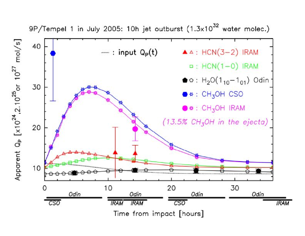
Figure 12: Same as in Fig. 11 for a release lasting 10 h.

Figure 16: Apparent H₂O production rates measured from Odin observations and the least squares fit of $Q/r_{h}^{2}$ to the data.

References

- [A’Hearn et al. 2005] A’Hearn, M. F., Belton, M. J. S., Delamere, W. A. and Blume, W. H., 2005a, Deep Impact: a large-scale active experiment on a cometary nucleus. Space Science Reviews, 117, 1–21
- [A’Hearn et al. 2005] A’Hearn, M. F., and 32 colleagues., 2005b, Deep Impact: Excavating Comet Tempel 1. Science, 310, 258–264
- [Altenhoff et al. 1987] Altenhoff, W. J., Baars, J. W. M., Wink, J. E. and Downes, D., 1987, Observations of anomalous refraction at radio wavelengths. Astron. Astrophys., 184, 381–385.
- [Beer et al. 2006] Beer, E.H., Podolak, M. and Prialnik, D., 2006, The contribution of icy grains to the activity of comets. I. Grain lifetime and distribution. Icarus, 180, 473–486
- [Belton et al.] Belton, M. J. S., and 15 colleages, 2005, Deep Impact: working properties for the target nucleus – comet 9P/Tempel 1. Space Science Reviews, 117, 137–160
- [Bensch et al. 2006] Bensch, F., Melnick, G.J., Neufeld, D.A., Harwit, M., Snell, R.L., Patten, B.M. and Tolls V., 2006, Submillimeter Wave Astronomy Satellite observations of Comet 9P/Tempel 1 and Deep Impact. Icarus, 184, 602–610
- [Biver (1997)] Biver, N., 1997, Molécules Mères cométaires: observations et modélisations. Ph.D. Thesis, Université Paris VII
- [Biver et al. 1999] Biver, N., and 13 colleagues, 1999, Spectroscopic Monitoring of Comet C/1996 B2 (Hyakutake) with the JCMT and IRAM Radio telescopes. Astron. J., 118, 1850–1872
- [Biver et al. 2000] Biver, N., and 12 colleagues, 2000, Spectroscopic observations of comet C/1999 H1 (Lee) with the SEST, JCMT, CSO, IRAM, and Nançay radio telescopes. Astron. J., 120, 1554–1570
- [Biver et al. 2002] Biver, N., Bockelée-Morvan, D., Croviser, J., Colom, P., Henry, F., Moreno, R., Paubert, G., Despois, D., and Lis, D. C., 2002, Chemical composition diversity among 24 comets observed at radio wavelengths. Earth Moon and Planets, 90, 323–333
- [Biver et al. 2005] Biver, N., Bockel e-Morvan, D., Colom, P., Crovisier, J., Lecacheux, A., and Paubert, G., 2005, Comet 9P/Tempel. IAU Circ. 8538
- [Biver et al. 2006a] Biver, N., Bockelée-Morvan, D., Crovisier, J., Lis, D.C., Moreno, R., Colom, P., Henry, F., Herpin, F., Paubert, G., and Womack, M., 2006a, Radio wavelength molecular observations of comets C/1999 T1 (McNaught-Hartley), C/2001 A2 (LINEAR), C/2000 WM1 (LINEAR) and 153P/Ikeya-Zhang. Astron. Astrophys., 449, 1255–1270
- [Biver et al. 2006b] Biver, N., Bockelée-Morvan, D., Crovisier, J., Lecacheux, A., Frisk, U., Hjalmarson, Å., Olberg, M., Florén, H. G., Sandqvist, Aa., and Kwok, S., 2006b, Submillimetre observations of comets with Odin: 2001–2005. Planet. Space Sci., In press
- [Bockelée-Morvan 1987] Bockelée-Morvan, D., 1987, A model for the excitation of water in comets. Astron. Astrophys., 181, 169–181
- [Bockelée-Morvan et al. 2004] Bockelée-Morvan, D., Biver, N., Colom, P., Crovisier, J., Henry, F., Lecacheux, A., Davies, J. K., Dent, W. R. F., and Weaver, H. A., 2004, The outgassing and composition of Comet 19P/Borrelly from radio observations. Icarus, 167, 113–128
- [Colom and Gérard 1988] Colom, P. and Gérard, E., 1988, A search for periodicities in the OH radio emission of comet P/Halley (1986 III). Astron. Astrophys., 204, 327–336
- [Colom et al. 2004] Colom, P., Biver, N., Crovisier, J., Lecacheux, A., and Bockelée-Morvan, D., 2004, Water outgassing rates in comets with ODIN and the Nançay Radio Telescope. In: SF2A-2004: Semaine de l’Astrophysique Francaise, EdP-Sciences, Conference Series, 69
- [Crovisier et al.] Crovisier, J., Colom, P., Gérard, E., Bockelée-Morvan, D., and Bourgois, G., 2002, Observations at Nançay of the 18-cm lines in comets The data base. Observations made from 1982 to 1999. Astron. Astrophys., 393, 1053–1064
- [Crovisier et al.] Crovisier, J., Colom, P., Biver, N., Bockelée-Morvan, D. and Lecacheux, A., 2005, Comet 9P/Tempel. IAU Circ. No 8512.
- [Despois et al.] Despois, D., Gérard, E., Crovisier, J. and Kazès, I, 1981, The OH radical in comets - Observation and analysis of the hyperfine microwave transitions at 1667 MHz and 1665 MHz. Astron. Astrophys., 99, 320–340
- [Frisk et al. 2003] Frisk, U., and 50 colleagues, 2003, The Odin satellite. I. Radiometer design and test. Astron. Astrophys., 402, L27–L34
- [Hjalmarson et al. 2003] Hjalmarson, Å., and 57 colleagues, 2003, Highlights from the first year of Odin observations. Astron. Astrophys., 402, L39–L46
- [Howell et al. 2005] Howell, E.S., Lovell, A.J., Butler, B. and Schloerb, F P., 2005, Radio OH observations of comet 9P/Tempel 1 before and after Deep Impact. Bull. Am. Astron. Soc. 37, 712
- [Jehin et al. 2006] Jehin, E., Manfroid, J., Hutsemékers, D., Cochran, A. L., Arpigny, C., Jackson, W. M., Rauer, H., Schulz, R., and Zucconi, J.-M., 2006, Deep Impact : High Resolution Optical Spectroscopy with the ESO VLT and the Keck 1 telescope. Astrophys. J. Letters, 641, L145–L148
- [Keller et al. 2005] Keller, H. U. Jorda, L., Küppers, M., Gutierrez, P. J., Hviid, S. F., Knollenberg, J., Lara, L.-M., Sierks, H., Barbieri, C., Lamy, P., Rickman, H., and Rodrigo, R., 2005, Deep Impact Observations by OSIRIS Onboard the Rosetta Spacecraft. Science, 310, 281–283
- [Küppers et al. 2005] Küppers, M., and 16 colleagues, 2005, A large dust/ice ratio in the nucleus of comet 9P/Tempel 1. Nature, 437, 987–990
- [Lisse et al.] Lisse, C. M., A’Hearn, M. F., Farnham, T. L., Groussin, O., Meech, K. J., Fink, U., and Schleicher, D. G., 2005, The coma of comet 9P/Tempel 1. Space Science Reviews, 117, 161–192
- [Meech et al. 2005a] Meech, K. J., A’Hearn, M. F., Fern ndez, Y. R., Lisse, C. M., Weaver, H. A., Biver, N., and Woodney, L. M., 2005a, The Deep Impact Earth-Based Campaign. Space Science Reviews, 117, 297–334
- [Meech et al. 2005b] Meech, K. J., and 208 colleagues, 2005b, Deep Impact: Observations from a Worlwide Earth-Based Campaign. Science, 310, 265–269
- [Mumma et al. 2005] Mumma, M. J., and 13 colleagues, 2005, Parent Volatiles in Comet 9P/Tempel 1: Before and After Impact. Science, 310, 270–274
- [Nordh et al. 2003] Nordh, H.L., and 17 colleagues, 2003, The Odin orbital observatory. Astron. Astrophys., 402, L21–L25
- [Olberg et al. 2003] Olberg, M., and 15 colleagues, 2003, The Odin satellite. II. Radiometer data processing and calibration. Astron. Astrophys., 402, L35–L38
- [Schleicher and A’Hearn 1988] Schleicher, D. G. and A’Hearn, M. F., 1988 The fluorescence of cometary OH. Astrophys. J., 331, 1058–1077,
- [Schleicher et al. 2006] Schleicher, D. G., Barnes, K. L. and Baugh, N. F., 2006 Photometry and imaging results for comet 9P/Tempel 1 and Deep Impact: gas production rates, postimpact light curves, and ejecta plume morphology. Astron. J., 131, 1130–1137,
- [Schulz et al. 2006] Schulz, R., Owens, A., Rodriguez-Pascual, P. M., Lumb, D., Erd, C., and Stüwe, J.A., 2006 Detection of water ice grains after the DEEP IMPACT onto Comet 9P/Tempel 1. Astron. Astrophys., 448, L53–L56
- [Stellingwerf 1978] Stellingwerf, R.F, 1978 Period determination using phase dispersion minimization. Astrophys. J., 224, 953–960,