Numerical Modeling of the Radio Nebula from the 2004 December 27 Giant Flare of SGR 1806-20

Abstract

We use the relativistic hydrodynamics code Cosmos++ to model the evolution of the radio nebula triggered by the Dec. 27, 2004 giant flare event of soft gamma repeater 1806-20. We primarily focus on the rebrightening and centroid motion occurring subsequent to day 20 following the flare event. We model this period as a mildly relativistic ($\gamma\sim 1.07-1.67$) jetted outflow expanding into the interstellar medium (ISM). We demonstrate that a jet with total energy $\sim 10^{46}$ ergs confined to a half opening angle $\sim 20^{\circ}$ fits the key observables of this event, e.g. the flux lightcurve, emission map centroid position, and aspect ratio. In particular, we find excellent agreement with observations if the rebrightening is due to the jet, moving at $0.5c$ and inclined $\sim 0^{\circ}-40^{\circ}$ toward the observer, colliding with a density discontinuity in the ISM at a radius of several $10^{16}$ cm. We also find that a jet with a higher velocity, $\gtrsim 0.7c$, and larger inclination, $\gtrsim 70^{\circ}$, moving into a uniform ISM can fit the observations in general, but tends to miss the details of rebrightening. The latter, uniform ISM model predicts an ISM density more than 100 times lower than that of the former model, and thus suggests an independent test which might discriminate between the two. One of the strongest constraints of both models is that the data seems to require a non-uniform jet in order to be well fit.

1 Introduction

On Dec. 27, 2004 a giant flare (GF) of $\gamma$-rays was observed from soft gamma repeater (SGR) 1806-20. This GF, the largest $\gamma$-ray transient event ever observed from within our galaxy, was comprised of a 0.2 s burst so bright that it briefly saturated all $\gamma$ and X-ray detectors in the solar system, followed by a several 100 s fading X-ray transient (Hurley et al., 2005). Such an outburst is thought to derive from a cataclysmic reorganization of the surface magnetic field of the magnetar, a neutron star distinguished by its exceptionally high surface magnetic field, $\sim 10^{15}$ G (Duncan & Thompson, 1992), which is the source of the SGR.

What is more, about one week after the GF a radio nebula was observed at the location of the SGR (Gaensler et al., 2005). Over the next couple of months this radio nebula was seen to expand and move across the sky (Taylor et al., 2005; Gelfand et al., 2005). The observations suggest two epochs of evolution. Epoch I spanned from the first detection of this radio afterglow about 7 days after the flare event to about 20 days post flare. This epoch was distinguished by a steep decay in observed flux ($\sim t^{-2.7}$), a slight motion of the flux centroid toward the West, and the detection of polarization of a few percent (Gaensler et al., 2005). Also, the nebula was observed to be elongated along the direction of motion with a roughly 2:1 aspect ratio. As pointed out by several authors, this epoch had interesting substructure, including a steepening of, or break in, the flux decay rate at $\sim 9$ days as well as variation in amplitude and pitch angle of observed polarization (Gelfand et al., 2005; Taylor et al., 2005; Cameron et al., 2005). The observation of polarization is indicative of some global order to the magnetic field hosting the synchrotron electrons.

Epoch II, commencing at about 20 days, was distinct from Epoch I in several ways. First, a rapid rebrightening occurred, followed by a shallower flux decay law ($\sim t^{-1.1}$) that persisted for the remainder of the reported observations, until $\sim 80$ days. Secondly the centroid of the flux began to move rapidly toward the Northwest. Also, polarization abruptly vanished, with no significant detections during this entire period, indicating a separate and distinct population of radiating electrons from that of Epoch I (Gelfand et al., 2005; Taylor et al., 2005).

The detection of proper motion of the emission source strongly suggests some sort of asymmetry. This asymmetry could be rooted in i) the ejected material having a particular direction, or ii) the surrounding environment having a particular shape. While nature might easily incorporate both components, the models proposed thus far, including the bulk of our work here, fall into the former category. We have, however, briefly explored the latter possibility by simulating a spherical isotropic mass ejection event centered in a cylindrical, evacuated cavity. This geometry mocks up the cavity that could be swept out by the SGR’s spin-down luminosity as it moves through the interstellar medium (ISM). In this model, the source of asymmetry would be the unhindered propagation of ejecta down the cylinder, in contrast to the ejecta colliding with its wall. Instead, the result we found was that the ejecta progressing down the cylinder, diminishing as $1/r^{2}$, is quickly dwarfed by the nearly isotropic external shock. Thus any early asymmetry is washed out. As such, this model makes the strong prediction that the flux centroid should return to the position of the SGR after some time. Since this has not been observed to happen for SGR 1806-20, such a model is disfavored.

The rest of the paper is organized into four sections. We begin by describing the models we wish to investigate and frame the parameter space to be explored with some theory, §2. In particular, we study two distinct models for the emission of Epoch II: collisional brightening, §2.1, in which this epoch commences when ejecta collides and shocks with a density step in the ISM, and doppler brightening, §2.2, for which the ejecta’s motion through a uniform ISM, and its progressive shocking and decelaration, is responsible for the Epoch II rebrightening. The latter model is most similar to that put forward by Granot et al. (2006), except that we assume Epoch I is independent of Epoch II (see §2). We also investigate structured jets §2.3 which we find to play a surprisingly important and interesting role in fitting the data. We then describe our numerical modeling method, §3, including our novel approach to post-processing observations from the data, §3.1. We describe our results in §4. While we find that both models studied are viable, the collisional brightening model, §4.1, does a better job than the doppler brightening model, §4.3, of fitting the data, particularly that of the lightcurve and centroid position. Of particular note, we find that structured jets, §4.2, rather than uniform jets, are required to fit the data for both models. Finally, we discuss our results and further ways these two models might be tested, §5.

2 The Models

In this paper we model the observations of the radio nebula from the Dec. 27, 2004 event. In particular we focus on Epoch II, defined by the rebrightening of radio flux and proper motion of its centroid and assume it to be distinct and independent of the emission of Epoch I. We adopt the natural hypothesis that Epoch II is the result of the interaction of material ejected during the GF event with an external, interstellar medium (ISM) (Gelfand et al., 2005; Taylor et al., 2005; Granot et al., 2006). Our goal is to understand and constrain how this interaction might have transpired. In particular, we attempt to address four key issues a) the rapid acceleration of the centroid motion, commencing at $\sim 20$ days, b) the rapid transition, $\Delta t_{pk}\sim 10$ days, from rise to decay of the rebrightening peak, c) the final decay slope $\propto t^{-1.1}$, and d) the observed 2:1 aspect ratio of the elongated emission ellipse, with major axis along the direction of centroid proper motion.

Figure 1: 4.8 GHz data (Gelfand et al., 2005) scaled to 8.5 GHz data (Taylor et al., 2005) by $F_{4.8}/F_{8.5}=1.5$, implying $F_{\nu}\propto\nu^{-0.6}$. This scaled 4.8 GHz is denoted with an asterisk (^∗) throughout this paper.

To address these issues we begin by assuming two independent flux components. The first gives rise to the Epoch I radio flux, independent of that of Epoch II, and can be described as a stationary point source at the location of the SGR, empirically parameterized as a decaying power-law

$$F_{\mathrm{I}}(t)\equiv 12\ \biggl{(}\frac{\nu}{8.5\mathrm{GHz}}\biggr{)}^{-0.6}\biggl{(}\frac{t}{\mathrm{day}}\biggr{)}^{-2.7}\quad\mathrm{Jy}~{},$$ (1)

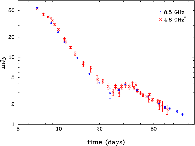
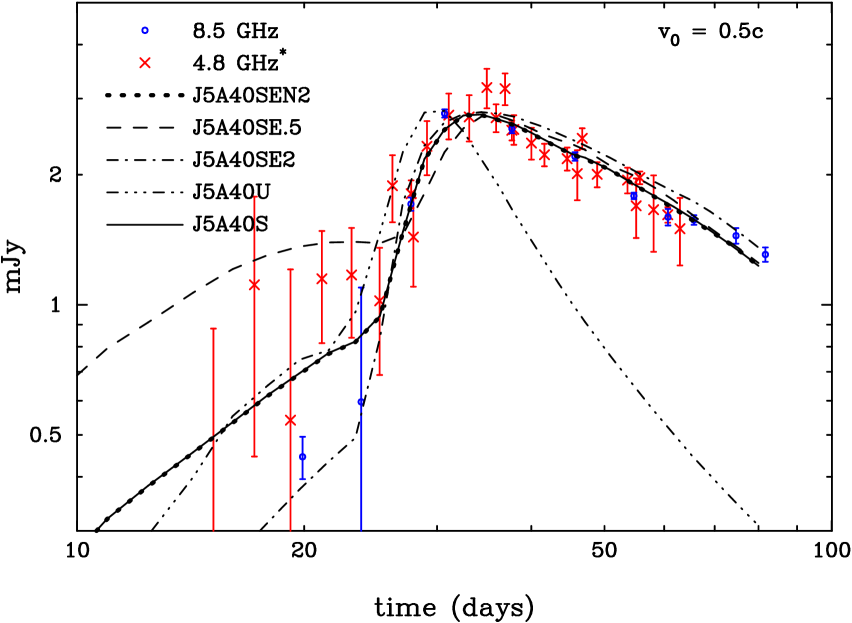
where the frequency dependence is motivated by Figure 1. We also assume that this flux component is present throughout all observations and both epochs, but will be referred to as the Epoch I flux component. While invoking equation 1 might gloss over the previously mentioned substructure evident at early times, we argue that this approximation is adequate and necessary to address its later interaction with Epoch II. For example, while there was a suggestion of proper motion of the radio nebula during Epoch I, it was not monotonic, but instead the centroid returned to effectively zero offset; nor was the motion in the same direction as the proper motion of Epoch II, and thus was not obviously directly related. The second flux component, designated Epoch II, is entirely derived from the shock interaction of ejecta emitted during the GF with the ISM. We wish to test the extent to which this simple two-component model can describe the data.

The assumption of a two-component model is a departure from that put forward by Granot et al. (2006), which proposes that the Epoch I emission component is due to the collision of the ejecta with the ISM at some time prior to the first observation at 6.9 days. For the reasons enumerated above, we interpret Epoch I to be physically distinct from Epoch II. This assumption is further bolstered by the observation that the distance the centroid has moved away from the location of the SGR is correlated with the size of the semi-major axis along the same direction, suggesting that the SGR continues to contribute to the flux throughout Epoch II.

Within this two flux component framework, our investigation forks into two branches. The first explores collisionally brightened flux in Epoch II, whereby the material ejected in the GF coasts largely unhindered until hitting a discontinuous jump or wall in the ISM, which induces a strong shock and rapid flux brightening. The second branch is Doppler brightening, whereby the GF ejecta is thought to have intercepted the ISM prior to the first observation ($\sim 7$ days) and thus will coast, brightening as it expands $\sim r^{2}$, until exhausting its initial kinetic energy to shocked internal energy, at which time it begins decelerating. This model is most like that proposed by Granot et al. (2006) except that they propose the shock due to the initial collision ($<7$ days) might account for Epoch I. Such a prediction does not naturally flow from our simulations; although we do model the ejecta colliding with the ISM at an early time, $r_{wall}/v_{0}\approx 6$ days (Table 1), and self-consistently calculate any flux deriving from that collision, we find any such flux to be negligible. Efforts to increase the ISM wall density, $n_{wall}$, were not successful in generating a non-negligible early flux component, but instead would significantly impact the ejecta mass and thus alter the conditions of the later evolution. Since the focus of this paper is on the later evolution of Epoch II, we assume the two flux components to be independent.

2.1 Collisional Brightening Model

Now we use the empirical emission model for Epoch I (equation 1) to place constraints on the size and shape of the emission of Epoch II. At the time of peak brightness of Epoch II, $t_{pk}\approx 30$ days, the flux centroid was offset from the SGR position by $d_{c}\approx 130$ mas. This is the mean position of both the flux with zero offset, $d_{I}=0$, from the SGR, $F_{I}(t)$, and the flux from the shocked, ejected material, $F_{II}$

$$d_{c}=\frac{d_{II}F_{II}}{F_{I}+F_{II}}\approx 130\biggl{(}\frac{Z_{\mathrm{obs}}}{15\mathrm{kpc}}\biggr{)}\ \mathrm{mas}~{}.$$ (2)

From equation 1, $F_{I}(t_{pk})=1.2$ mJy at 8.5 GHz and using the data by Taylor et al. (2005), the total flux was $F_{I}+F_{II}=3.9$ mJy. Thus we get an estimate for the observed position of the ejected shock at peak brightness (when it is beginning to decelerate)

$$d_{II}=\frac{F_{I}+F_{II}}{F_{II}}d_{c}=1.4\times 130\ \mathrm{mas}=0.52\biggl{(}\frac{Z_{\mathrm{obs}}}{15\mathrm{kpc}}\biggr{)}\ \mathrm{light-months}~{}.$$ (3)

Thus we estimate the projected velocity of the ejected material across the sky to be $d_{II}/t_{pk}\approx 0.5c$. The projected distance, $d$, moved by an object over an observer interval, $t_{obs}$, can be related to the material’s true initial velocity, $v_{0}$, and inclination angle, $\theta_{i}$, with respect to image plane ($\theta_{i}>0$ is inclined toward the observer) by

$$t_{obs}=(1-(v_{0}/c)\sin\theta_{i})\frac{d}{v_{0}\cos\theta_{i}}$$ (4)

and therefore a relationship between the true velocity and inclination is given by

$$v_{0}(\theta_{i})=\frac{c}{\sin\theta_{i}+(c/v_{\perp})\cos\theta_{i}}$$ (5)

where $v_{\perp}\equiv d/t_{obs}$. This equation suggests that if $v_{\perp}=d_{II}/t_{pk}\approx 0.5c$, then $v_{0}\sim v_{\perp}$ within $10\%$ for $0^{\circ}\lesssim\theta_{i}\lesssim 60^{\circ}$, but increases rapidly to $c$ for inclination angles approaching $90^{\circ}$. Finally, the characteristic true distance from the SGR at which the ejecta peaked in brightness was

$$R=\frac{d_{II}}{\cos\theta_{i}}~{}.$$ (6)

Another interesting constraint is the swiftness with which the Epoch II flux rebrightening increased, peaked, and began to decay. This entire transition happened within a time span of $\Delta t_{pk}\sim 10$ days $\sim t_{pk}/3$. If we assume that the peak of emission corresponds to a self-similar Sedov-Taylor blastwave reaching its deceleration radius, then we generally expect $\Delta t_{pk}\sim t_{pk}$, i.e. it is difficult to make temporal features shorter than the blastwave timescale. In our case we assume the emission derives from a jet with radial opening angle, $\theta_{0}$, measured from its axis. Thus we may estimate this timescale as simply the timespan between when the observer first sees the nearest (“front”) edge and the furthest (“back”) edge of the jet reach a characteristic radius, $R$. Using equation 4 gives

$$\Delta t_{pk}=t_{b}-t_{f}=\frac{R}{c}(\sin\theta_{f}-\sin\theta_{b})=2\frac{d_{II}}{c}\sin\theta_{0}$$ (7)

where $\theta_{f}\equiv\theta_{i}+\theta_{0}$ and $\theta_{b}\equiv\theta_{i}-\theta_{0}$. Surprisingly, this result is independent of the derived quantities $R$ and $\theta_{i}$ and allows one to solve for the opening angle as a function only of observed quantities

$$\theta_{0}=\arcsin\biggl{(}\frac{c\Delta t_{pk}}{2d_{II}}\biggr{)}\approx 20^{\circ}\biggl{(}\frac{0.5c}{v_{\perp}}\biggr{)}\biggl{(}\frac{15\mathrm{kpc}}{Z_{\mathrm{obs}}}\biggr{)}~{}.$$ (8)

If, as has been suggested (Taylor et al., 2005), the front of the jet moves at twice the velocity of the centroid, i.e. $v_{\perp}=2\times d_{c}/t_{pk}\sim 0.7c$, then we expect the opening angle to be $\theta_{0}\sim 14^{\circ}$.

2.2 Doppler Brightening Model

The rapid peaking of Epoch II can also provide a constraint on the angle of inclination and ejecta velocity if we assume that this transition is due only to the ejecta beginning to decelerate as it moves into, and sweeps up the interstellar medium. This is distinct from the model described in the previous section in which the rapid rise in flux of Epoch II is due to the collision of the ejecta with a discontinuous rise in external density. As previously mentioned, due to the self-similar nature of this expansion, we expect the time to peak $t_{pk}\propto r_{dec}/v_{0}\sim\Delta t_{pk}$, where the deceleration radius, at which the ejecta has expended its expansion energy by shocking the external medium, scales like $r_{dec}\propto[E_{0}/(n_{ext}v_{0}^{2})]^{1/3}$, where $E_{0}$ is the ejecta energy and $n_{ext}$ is the density of the external medium. If the observed temporal shortening is assumed to be due entirely to Doppler blue shift, then the observation $\Delta t_{pk}\sim t_{pk}/3$ implies $(1-v_{0}\sin\theta_{i})\sim 1/3$, where $t_{pk}=d/(v_{0}\cos\theta_{i})$. Then using equations 4 and 6 we have

$$t_{obs}=(1-v_{0}\sin\theta_{i})\biggl{(}\frac{r_{dec}}{v_{0}}\biggr{)}\approx\text@frac{1}{3}\biggl{(}\frac{r_{dec}}{v_{0}}\biggr{)}$$ (9)

and assuming the proper motion of the head of the jet is twice the value of the centroid

$$v_{\perp}=\frac{r_{dec}\cos\theta_{i}}{t_{pk}}=\frac{2d_{c}}{t_{pk}}\approx 0.7c$$ (10)

allows us to solve for the inclination and velocity uniquely

$$\theta_{i} = 70^{\circ}$$ (11)

$$v_{0} = 0.7c~{}.$$

This allows us to estimate the deceleration radius, $r_{dec}=2d_{c}/\cos\theta_{i}\approx 1.7\times 10^{17}$ cm (eqn. 10) at an observed distance $Z_{\mathrm{obs}}=15$ kpc. Using this information and the aforementioned estimate of opening angle, $\theta_{0}$, we can find the total energy of the ejecta as a function of external, interstellar density; $\rho_{ext}=n_{ext}m_{p}c^{2}$. To do so we note that at the deceleration radius the initial kinetic energy, $E_{k}$, of the ejecta has been exhausted by shocking the external medium

$$E_{k}\approx\frac{\pi\theta_{0}^{2}}{3}r^{3}_{dec}\rho_{ext}c^{2}(\gamma-1)(1+\Gamma(\gamma-1))$$ (12)

where the shocked medium is boosted by the Lorentz factor $\gamma\equiv(1-v_{0}^{2})^{-1/2}$ and the factor $(1+\Gamma(\gamma-1))$ is the specific enthalpy of the shocked external medium (e.g. Anninos et al., 2005) and here we take $\Gamma=5/3$. Since we assume the initial ejecta material is cold, the total energy is related to the mass as $E_{0}=\gamma M_{0}c^{2}$ and the kinetic energy as $E_{k}=(\gamma-1)M_{0}c^{2}$, so $E_{0}=E_{k}/(1-1/\gamma)$ and

$$E_{0}\approx 1\times 10^{48}\biggl{(}\frac{\theta_{0}}{14^{\circ}}\biggr{)}^{2}\biggl{(}\frac{n_{ext}}{1~{}\mathrm{cm}^{-3}}\biggr{)}~{}\mathrm{ergs}~{}.$$ (13)

This is a remarkably simple formula for the total energy of the GF ejecta and is determined entirely from kinematic arguments. It is independent of radiative efficiency factors which plague most energy estimations. We have numerically simulated a jet with the parameters of eqn. 11, iterating to find the best fit to the observations for our adopted radiation parameters (see §3.1.2). Our best fit is J7UHI (Table 1). From the table we find $\theta_{0}=12^{\circ}$ and $n_{ext}=0.003$ cm^-3, for which eqn. 13 gives $E_{0}=0.23\times 10^{46}$ ergs, which is about three times lower than the actual value from the table as taken from the simulation. Given the sensitive dependence of $r_{dec}$ on $\theta_{i}$, this difference in total energy measurements corrsponds to $\sim 6^{\circ}$ uncertainty in $\theta_{i}$. This uncertainty is significantly less than the jet opening angle, $\theta_{0}$, and thus is within the uncertainty of the location of maximum emission, due to Doppler effects, on the shock front. Therefore we find the simple eqn. 13 to be tolerably accurate and insightful expression for the Doppler brightening model.

2.3 Structured Jets

A key point of this study is to explore possible jet structures and their effects on observables. The physical motivation for this is clear; nature need not contrive that the material was ejected in the SGR as a uniform pancake with a distinct edge. The actual morphology of the ejecta is an open question and, as it pertains to gamma-ray burst afterglows, has been studied by several authors (Salmonson & Galama, 2002; Rossi et al., 2002; Kumar & Granot, 2003; Salmonson, 2003; Rossi et al., 2004).

We study three basic jet morphologies, all characterized by an opening angle $\theta_{0}$ measured from the jet axis. The “uniform” jet is the simplest, where the ejecta mass density, $\rho$, and initial velocity, $v_{0}$, are constants for the region $\theta<\theta_{0}$, but are both otherwise zero. The “power-law” jet is constructed by multiplying the ejecta mass density by the angle factor

$$\mathcal{A}_{P}(\theta)\equiv\frac{1}{1-(\theta/\theta_{0})^{2}}$$ (14)

and the velocity is $v(\theta)=v_{0}\mathcal{A}^{s}_{P}(\theta)$, where $s$ is typically between $0.5-1.0$. The “gaussian” jet multiplies the mass density by

$$\mathcal{A}_{G}(\theta)\equiv\exp\biggl{[}-\text@frac{1}{2}\biggl{(}\frac{\theta}{\theta_{0}}\biggr{)}^{2}\biggr{]}$$ (15)

and the velocity is $v(\theta)=v_{0}\mathcal{A}^{s}_{G}(\theta)$. These three jet types are indicated by a “U”, “P”, or “G” respectively in Table 1 and the power of the velocity factor, $s$, is unity unless otherwise given in parenthesis.

3 Numerical Modeling: Cosmos++ 

In this paper we report numerical simulations using Cosmos++ , a recently completed multidimensional, radiation-chemo-magnetohydrodynamic code for both Newtonian and (general) relativistic flows. The capabilities and tests of Cosmos++ are described in (Anninos et al., 2005). This code represents a significant advance over our previous numerical code (Cosmos; Anninos & Fragile, 2003), with improvements in ultra-relativistic shock-capturing capabilities, regularization of the symmetry axis, more accurate energy conserving methods, and adaptive mesh refinement (AMR). The mildly relativistic flows considered in this paper require accurate relativistic hydrodynamical capabilites and substantial resolution to resolve the narrow, length-contracted shock fronts and flow features. Thus this present work requires of all of these features and advances.

The simulations are performed using special relativistic hydrodynamics and are initialized with a cold shell of ejecta mass $M_{0}$, and total energy $E_{0}$ at radius $r_{0}$ from the SGR moving with an initial radial speed $v_{0}$. Since the ejecta exhibited motion in a particular direction, we take the shell to be an axisymmetric jet with a characteristic radial opening angle $\theta_{0}$ from the jet axis. This angle, $\theta_{0}$, is either a distinct edge to a uniform jet, or might be a characteristic angle over which density and/or velocity vary as a function of angle from a structured jet axis, as was discussed in detail in §2.3. The shell thickness is constrained to be $\sim 1$ light-hour, corresponding to the minimum zone size of the refined grid. If the ejecta is linked to the GF event it was likely ejected on a much shorter timescale, perhaps seconds, which is consistent with the idea that, since the ejecta appears to have a specific direction, it must have been ejected over a fraction of a rotation period, $7.6~{}s$, of the SGR unless it was ejected along the rotation axis. However, there was likely a dispersion to the ejecta velocity, or a temperature in the gas, so the shell would likely have expanded significantly over the ensuing days as it coasted. Thus our initial shell width is not unreasonable.

The simulations are initiated on a two-dimensional ($r$, $\theta$) base grid with a typical resolution: $108\times 24$. The grid covers the spatial domain $0.01\lesssim r\lesssim 0.4$ light-years, and $0\leq\theta\leq\pi/3,~{}\pi/4$ or $\pi/6$, with a reflective boundary at $\theta=0$. The resolution of the base grid is $\Delta r\approx 1$ light-day. Four to six levels of refinement are allowed on this base grid during the evolution. The refinement and derefinement criteria are described in Anninos et al. (2005) and use the magnitude, slope, and curvature of the density field to ensure that the Lorentz-contracted shell of the blast wave is always maximally resolved, while low density background regions in the flow are minimally resolved. At maximum refinement, the resolution is $\Delta r\approx 1$ light-hour or better. The simulations cover a time span from $t=5-10$ days to $t=75-200$ days.

3.1 Post Processing

A key step in assessing the merits of a particular simulation is the extraction of observable attributes which can be compared with actual observations. In this case we are interested in simulating observations at radio wavelengths. To do this we create synthetic radio intensity “images” for a specified frequency at several observer times. From these can be obtained an observed flux for that frequency and time as well as the position and shape of the emitting region; all of these data were observed for the radio afterglow of the 27 Dec 04 giant flare and can thus be compared.

3.1.1 Radiative Transfer

In Cosmos++ the relativistic hydrodynamic equations are integrated along parallel time slices, so that for a problem state at a given simulation (laboratory) time, $t$, all positions, $(x,y,z)$, on the mesh are simultaneous in time. In this case the laboratory frame is such that the SGR at the coordinate origin is stationary and so, to an excellent approximation, is the terrestrial observer. If, say, the observer is located at some large distance $Z_{\mathrm{obs}}$ along the $z$-axis, then he will observe light from the object that is essentially parallel to the $z$-axis. Thus the observer’s spatial coordinates $(x_{\mathrm{obs}},y_{\mathrm{obs}},z_{\mathrm{obs}})$ perceived simultaneously at time $t_{\mathrm{obs}}$ will transform from those of the simulation simply as

$$(t_{\mathrm{obs}},x_{\mathrm{obs}},y_{\mathrm{obs}},z_{\mathrm{obs}})=(t-z/c,x,y,z)-(Z_{\mathrm{obs}}/c,0,0,Z_{\mathrm{obs}})+(r_{0}/v_{0},0,0,0)~{},$$ (16)

where the last two terms are arbitrary, constant origin offsets. The middle term corresponds to look-back time from the Earth and will be neglected. The last term accounts for the fact that the simulation is started (at $t=0$) after the ejecta, moving at some velocity $v_{0}$, has moved a distance $r_{0}$ from the SGR.

To construct a flux map at a given observer frequency, $\nu$, and time, $t_{\mathrm{obs}}$, we integrate the radiative transfer equation through the simulation data, along the z-axis toward the observer

$$I_{\nu}(t_{\mathrm{obs}},x_{\mathrm{obs}},y_{\mathrm{obs}},Z_{\mathrm{obs}})=\int(j_{\nu}-\alpha_{\nu}I_{\nu})dz_{\mathrm{obs}}~{},$$ (17)

where $I_{\nu}$ is the intensity, $j_{\nu}$ the emissivity, and $\alpha_{\nu}$ the opacity of the material at a position $(t_{\mathrm{obs}},x_{\mathrm{obs}},y_{\mathrm{obs}},z_{\mathrm{obs}})$. Finally, the observed flux is given by

$$F_{\nu}(t_{\mathrm{obs}},Z_{\mathrm{obs}})=\int\int I_{\nu}(t_{\mathrm{obs}},x_{\mathrm{obs}},y_{\mathrm{obs}},Z_{\mathrm{obs}})\times\frac{dx_{\mathrm{obs}}dy_{\mathrm{obs}}}{Z^{2}_{\mathrm{obs}}}~{}.$$ (18)

Distance estimates to SGR 1806-20 have been in the range $12<Z_{\mathrm{obs}}<15$ kpc (Corbel & Eikenberry, 2004; Figer et al., 2005). See, however, the lower estimate of 9.8 kpc obtained from observations of absorption spectra of this GF event (Cameron et al., 2005). We take the high value of this range

$$Z_{\mathrm{obs}}\approx 15\mathrm{kpc}$$ (19)

as a worst case with respect to energy requirements, so that our reported flux and energy estimates might be relaxed by as much as a factor $~{}(9.8/15)^{2}\sim 0.4$, but are not likely to be tightened (see §3.2).

The emissivity and opacity, which are needed in the observer frame, are transformed from those calculated in the proper (rest) frame of the fluid, denoted by a prime, as (see eqns. 4.112 & 4.113 of Rybicki & Lightman, 1979)

$$\alpha_{\nu} \equiv \alpha(\nu)=\frac{\alpha^{\prime}(\nu^{\prime})}{\delta}=\frac{\alpha^{\prime}(\nu/\delta)}{\delta}~{},$$ (20)

$$j_{\nu} \equiv j(\nu)=\delta^{2}j^{\prime}(\nu^{\prime})=\delta^{2}j^{\prime}(\nu/\delta)~{}.$$

The proper frequency $\nu^{\prime}=\nu/\delta$ transforms with the Doppler factor defined as

$$\delta\equiv[\gamma(1-v_{z})]^{-1}~{},$$ (21)

where $v_{z}$ is the fluid velocity component along the z-axis (toward the observer), and $\gamma$ is the Lorentz factor

$$\gamma\equiv[1-\vec{v}\cdot\vec{v}]^{-1/2}~{}.$$ (22)

Thus we have a framework to simulate the observed intensity map and flux for any special relativistic simulation for which the proper radiation transport quantities $\alpha^{\prime}(\nu^{\prime})$ and $j^{\prime}(\nu^{\prime})$ can be determined locally from the state variables of the simulation. In the next section we describe this for the case of self-absorbed synchrotron radiation.

3.1.2 Self-Absorption Synchrotron Radiation

The observation of non-thermal (power-law) radio emission from the expanding nebula of this GF suggests synchrotron radiation from the electrons in the shocked material as the dominant emission mechanism. The standard theory of self-absorbed synchrotron emission has been presented in several works (e.g. Rybicki & Lightman, 1979; Chevalier, 1998; Li & Chevalier, 1999, and references therein). Our implementation of this basically standard model is presented here. The physical picture of this model is that hydrodynamic processes such as shocks will energize the plasma being simulated, thus accelerating its population of electrons into a power-law distribution as a function of Lorentz factor

$$n(\gamma)=C\gamma^{-p}~{},$$ (23)

starting from some minimum Lorentz factor $\gamma_{m}$. A key physical parameter is introduced by assuming that only a proportion, $\epsilon_{e}$, of the total proper energy density, $e^{\prime}=E/\gamma$ from the simulation, is represented in the electrons. Thus the fraction of energy in electrons is

$$\epsilon_{e}e^{\prime}=\int_{\gamma_{m}}^{\infty}(\gamma-1)m_{e}c^{2}n(\gamma)d\gamma~{}.$$ (24)

Plugging in equation 23, we can solve for the constant $C$

$$C=\frac{\epsilon_{e}e^{\prime}}{m_{e}c^{2}}\biggl{[}\frac{\gamma_{m}^{2-p}}{p-2}-\frac{\gamma_{m}^{1-p}}{p-1}\biggr{]}^{-1}~{}.$$ (25)

Another fundamental parameter of the model is the proportion, $\epsilon_{B}$, of the total energy density, $e^{\prime}$, manifest as magnetic field energy density, $B^{2}/8\pi$:

$$B=(8\pi\epsilon_{B}e^{\prime})^{1/2}~{}.$$ (26)

The synchrotron emission results from the population of electrons moving in, and being accelerated by the $B$-field. The relative orientation, or pitch angle, of an electron’s trajectory with respect to the $B$-field vector strongly effects the radiation. We treat this pitch angle in an average sense by following the treatment of Wijers & Galama (1999). They calculate scaling factors such that the characteristic frequency emitted by a distribution of electrons (equation 23) in a field $B$ scales like

$$\nu^{\prime}_{m}\propto\chi_{p}B~{},$$ (27)

and the isotropic emission at that characteristic frequency will be

$$j^{\prime}(\nu^{\prime}_{m})\propto\phi_{p}B~{}.$$ (28)

We parameterize their functions of electron index $p$ (see Fig. 1 of Wijers & Galama, 1999)

$$\chi_{p} \approx p^{-3/2}+0.267~{},$$ (29)

$$\phi_{p} \approx 0.53\arctan(p)~{},$$

which give values $\chi_{p}(p=2.5)=0.52$ and $\phi_{p}(p=2.5)=0.63$.

So finally, we get for the opacity

$$\alpha^{\prime}(\nu^{\prime})=(m_{e}c^{2})^{p-1}\frac{\sqrt{3}q^{3}}{8\pi m_{e}}\biggl{(}\frac{3q}{2\pi m_{e}^{3}c^{5}}\biggr{)}^{p/2}C\ (\phi_{p}B)(\chi_{p}B)^{p/2}\Gamma\biggl{(}\frac{3p+2}{12}\biggr{)}\Gamma\biggl{(}\frac{3p+22}{12}\biggr{)}{\nu^{\prime}}^{-(p+4)/2}~{},$$ (30)

where $\Gamma()$ is Euler’s gamma function, $q$ the electron charge, and we note the factor $(m_{e}c^{2})^{p-1}$ is required to correct the dimensional inconsistency of the expression in Rybicki & Lightman (1979). The emmissivity is given by

$$j^{\prime}(\nu^{\prime})=\frac{\sqrt{3}q^{3}C\phi_{p}B}{(4\pi)2\pi m_{e}c^{2}(p+1)}\Gamma\biggl{(}\frac{p}{4}+\frac{19}{12}\biggr{)}\Gamma\biggl{(}\frac{p}{4}-\frac{1}{12}\biggr{)}\biggl{(}\frac{2\pi m_{e}c\nu^{\prime}}{3q\chi_{p}B}\biggr{)}^{-(p-1)/2}~{}.$$ (31)

The radiative properties of a parcel of shocked material from a simulation depends on the proper energy and velocity state variables of the plasma in the simulation, $(e^{\prime},\vec{v})$, as well as the emission modeling parameters $(p,\gamma_{m},\epsilon_{e},\epsilon_{B})$. The minimum electron Lorentz factor, $\gamma_{m}$, is typically assumed to be a few. For the wavelengths primarily considered here we don’t find particular sensitivity to this parameter, and so deem it sufficient to set it to $\gamma_{m}\approx 2$.

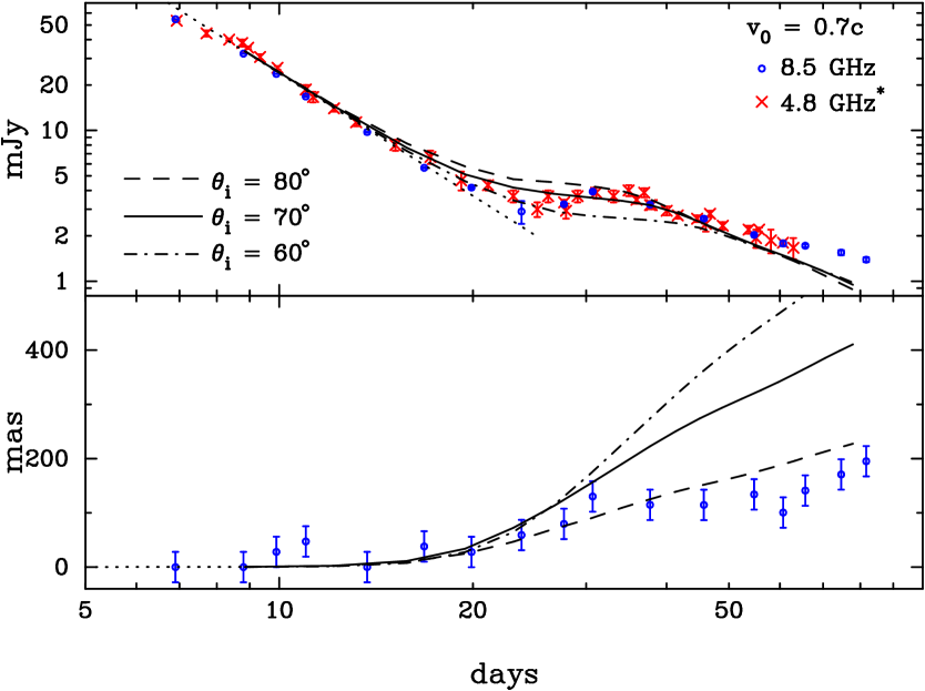
The electron index, $p$, impacts both the spectral and temporal decay slopes and therefore it is desireable to have an independent indication of its value. An intermediate result of this paper is that the 4.8 GHz (Gelfand et al., 2005) and 8.5 GHz data (Taylor et al., 2005) are consistent with $F_{4.8}/F_{8.5}\approx 1.5$ throughout the observational period (Figure 1). Furthermore, the single observation by Taylor et al. (2005) at 22.5 GHz at $\sim 23$ days is also consistent with the other points when scaled accordingly. This implies $F_{\nu}\propto\nu^{-0.6}\propto\nu^{-(p-1)/2}$ which, in turn implies

$$p\approx 2.2~{},$$ (32)

which is the value we use throughout this paper. While it is clear that detailed multiwavelength observations yield rich spectral substructure (Cameron et al., 2005) it is also the case that the shorter wavelengths, where we have the best chance at accurately modeling the emission, can be represented by a single electron index.

3.2 Comparison with Data

To fit the simulation to the data one must synchronize the simulation time and observer time by adding $r_{0}/v_{0}$ to the simulation time (equation 16) and then determine the normalization, $\mathcal{E}_{N}$ (Table 1), required to best match the flux magnitudes. In all of the models presented here and summarized in Table 1 (save the deliberate exceptions J5A40SE2, J5A40SE.5, J5A40SEN2) the simulations were calibrated to match the data as nearly as possible, so $\mathcal{E}_{N}$ can be thought of as a fine tuning parameter to match the data precisely.

Since we find the optical depth of these systems to be negligible, the magnitude of the flux has the dependence

$$F_{\nu}\propto j^{\prime}\propto\mathcal{E}_{N}\biggl{(}\frac{\epsilon_{e}}{0.1}\biggr{)}\biggl{(}\frac{\epsilon_{B}}{0.1}\biggr{)}^{(p+1)/4}\biggl{(}\frac{\nu}{\mathrm{8.5GHz}}\biggr{)}^{(1-p)/2}{e^{\prime}}^{(p+5)/4}~{},$$ (33)

where $e^{\prime}$ is the proper internal energy of the fluid in the simulation, $\epsilon_{e}$ and $\epsilon_{B}$ parameterize the amount of this energy in electrons and magnetic field respectively, and $\mathcal{E}_{N}$ is the final efficiency or normalization required to scale the simulated flux to that of the data. As denoted, throughout this paper we assume 10% of the energy is expressed in each the electrons and magnetic field.

A convenient and robust scaling can be applied to the interpretation of these simulation results. As discussed in §3, the initial ejecta energy, $E_{0}$, is deposited as a cold gas into a fixed volume (presumably constrained by the deposition timescale). Thus $E_{0}\propto\rho v_{0}^{2}$. Also, as the ejecta expands and shocks, it will heat according to $e^{\prime}\propto\rho v^{2}$. For a class of simulations in which a key hydrodynamic size scale is held fixed, i.e. the deceleration radius $r_{dec}\propto(E_{0}/n/v^{2}_{0})^{1/3}$, we have $n\propto E_{0}$ for a given $v_{0}$ and this enforces similar hydrodynamic evolution, $v\sim v_{0}(r_{dec}/r)^{-3/2}$. Thus for a given model, the shock heating scales with total energy; $e^{\prime}\propto E_{0}$. So the simulated flux scales as

$$F_{\nu} \propto j^{\prime}\propto\mathcal{E}_{N}\biggl{(}\frac{\epsilon_{e}}{0.1}\biggr{)}\biggl{(}\frac{\epsilon_{B}}{0.1}\biggr{)}^{(p+1)/4}\biggl{(}\frac{\nu}{\mathrm{8.5GHz}}\biggr{)}^{(1-p)/2}\biggl{(}\frac{Z_{\mathrm{obs}}}{15\mathrm{kpc}}\biggr{)}^{-2}{E_{0}}^{(p+5)/4}~{},$$ (34)

$$n \propto E_{0}~{},$$

where $n$ denotes all external number densities; $n_{ext},n_{int},n_{wall}$. For example, models J5A40S and J5A40SEN2 differ solely in that their total energy, $E_{0}$, and external densities $n_{ext},n_{int},n_{wall}$ are doubled in J5A40SEN2 from those in J5A40S. Equation 34 then suggests that J5A40SEN2 will have higher flux by a factor $2^{1.8}\approx 3.5$, using equation 32. Indeed, the ratio of factors $\mathcal{E}_{N}$ is precisely $1/3.5$ so that both simulations match the data (see Table 1). In fact, we show below that the resulting flux curves are indistinguishable from one another. Not only does this validate the hydrodynamic scaling expected from using a barotropic, $P\propto\rho^{\Gamma}$, equation of state, but also allows for convenient reinterpretation of the data. For instance, the factor, $\mathcal{E}_{N}$, can be used to scale $M_{0},E_{0},n_{ext},n_{int},n_{wall}$ by $\mathcal{E}_{N}^{4/(p+5)}$, or to scale one of the other terms in equation 34. Similarly, if an independent measurement were to constrain the external density or efficiency parameters, one can then calculate that effect on the other physical parameters. Alternative distances to the SGR (see discussion at equation 19) can be accommodated. The uncertainty in the emission physics parameters can be addressed by

$$E_{0}\propto n\propto\biggl{(}\frac{\epsilon_{e}}{0.1}\biggr{)}^{-4/(p+5)}\biggl{(}\frac{\epsilon_{B}}{0.1}\biggr{)}^{-(p+1)/(p+5)}~{}.$$ (35)

3.3 Aspect Ratio

One metric that can be used to compare the shape of the observed radio nebula to that of simulations is the aspect ratio. Observationally, this value is the ratio of minor to major axes of an ellipse fitted to the shape of the observed radio nebula. In order to make the most realistic comparison with observations possible, we begin with our simulated flux map $F_{\nu}$ given by equation 18 and convolve it with a 2D gaussian filter, $\propto\exp(-1/2(\varrho/\sigma)^{2})$ to blur the image (call it $F^{*}_{\nu}$) where $\varrho\equiv\sqrt{x^{2}+y^{2}}$. Herein we set $\sigma=50$ mas which is reasonable in that it blurs out small features while not significantly impacting the overall structure of the image. The aspect ratio of this blurred flux map, $F^{*}_{\nu}$, is then the ratio of the root mean square width to height defined by

$$\sqrt{\frac{<x^{2}>-<x>^{2}}{<y^{2}>-<y>^{2}}}$$ (36)

where

$$<\xi^{i}>\equiv\frac{\int\int\xi^{i}F^{*}_{\nu}dxdy}{\int\int F^{*}_{\nu}dxdy}$$ (37)

and $\xi=[x,y]$ and $i=[1,2]$.

4 Results

We present our results as a series of fits to observations in ascending order of initial ejecta velocity, $v_{0}$. For the collisional brightening models, the velocity range we examine begins at $v_{0}=0.35c\approx d_{c}/t_{pk}$ which is roughly the minimum velocity the ejecta could have had and still account for the observed centroid offset, $d_{c}\approx 130$ mas, and continues to $v_{0}=0.5c$, for which we find three example solutions. In the case of Doppler brightened models, we find higher velocities are required, specifically we consider models with $v_{0}=0.7c$ and $0.8c$.

4.1 Collisional Brightening Results

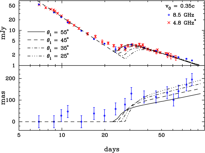
At the lowest ejection velocity we consider, $v_{0}=0.35c$, we demonstrate the effect on observations of inclination angle, $\theta_{i}$, of the jet axis out of the observer view plane. In Figure 2 one can see the sensitive dependence of the Epoch II flux on inclination; the lightcurve is advanced and doppler brightened as $\theta_{i}$ is increased. Note that all curves fall on the same decay law at late times, as expected due to the waning importance of doppler effects as the jet decelerates as noted previously in Salmonson (2003). By adding the Epoch I component (equation 1) one gets a total light curve and centroid offset prediction for this simulation, as seen at various inclinations in Figure 3. One can see that either the flux or centroid off-set curves can be fit reasonably well, but not both. To do so one must go to higher ejecta velocity.

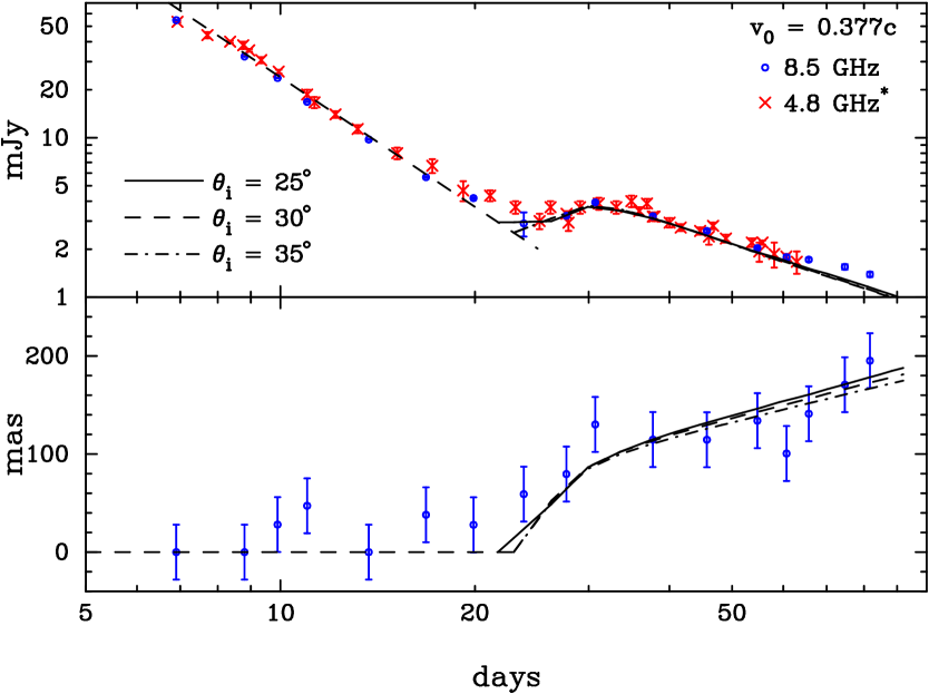
By increasing the ejecta velocity to $v_{0}=0.377c$ ($\gamma=1.08$) one can begin to come close to satisfying both the flux and centroid offset observations. In Figure 4 are shown three separate models, each individually tuned to best match the data. The tuning is rather crude, but a basic trend is highlighted. Increasing the density of the wall bounding the ISM, $n_{wall}$, or the region internal to it, $n_{int}$, causes a more rapid brightening of the Epoch II flux bump, which can then be compensated by reducing the inclination, $\theta_{i}$. Thus the morphology of the external medium is degenerate with the inclination angle. Note also that model J377I25, with a significant internal density, $n_{int}$, shows some brightening (and motion of its centroid) prior to collision with the wall. This qualitatively matches the data better and thus argues for a non-negligible internal medium.

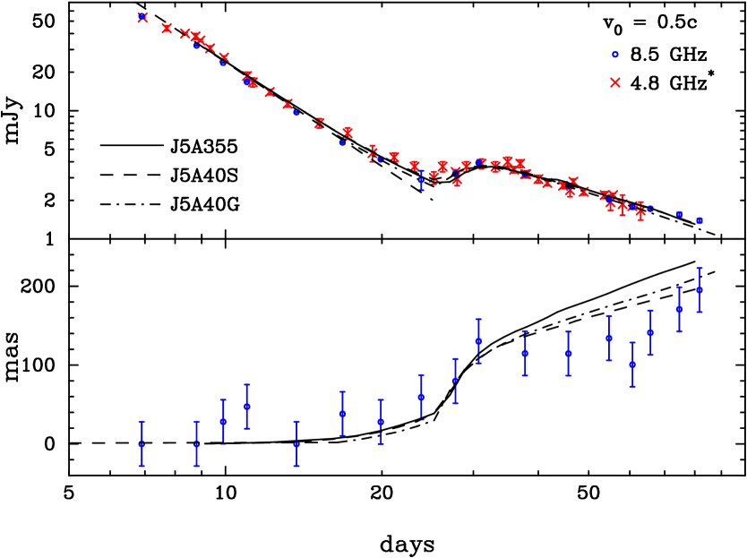
Next we consider $v_{0}=0.5c$. While the $v_{0}=0.377c$ case nominally satisfied the flux and centroid offset constraints, it was a bit shy in satisfying the observed centroid offset at 30 days. Figure 5 shows three individually tuned cases which each demonstrate good agreement with the data for $v_{0}=0.5c$. Of note is the $45^{\circ}$ deficit in inclination angle between model J5A355 and the other two. This low viewing angle is compensated for by reducing the wall radius, $r_{wall}$ and increasing its density $n_{wall}$ so the jet is seen to collide and brighten at the same time as the other models. The other models, J5A40S and J5A40G, contrast our two basic structural morphologies of the jet, with angular ejecta mass density variation described by equations 14 and 15 respectively. It is clear that each model can be tuned to fit the observations, thus making differentiation between the models impossible with present data. Figure 6 shows several different variation of model J5A40S, as well as uniform jet model J5A40U. The striking agreement of J5A40SEN2 and J5A40S speaks to the robust hydrodynamic scaling exhibited in these simulations, as discussed in §3.2. Varying the total energy $E_{0}$ by a factor 0.5 (J5A40SE.5) or 2 (J5A40SE2) gives an idea of how sensitive these solutions are to this parameter. The former(latter) case reduces(increases) the deceleration radius and thus increases(decreases) relative flux at early time. Finally, J5A40U demonstrates the stark difference in the uniform jet evolution to the other, structured jets. This will be discussed further in §4.2.

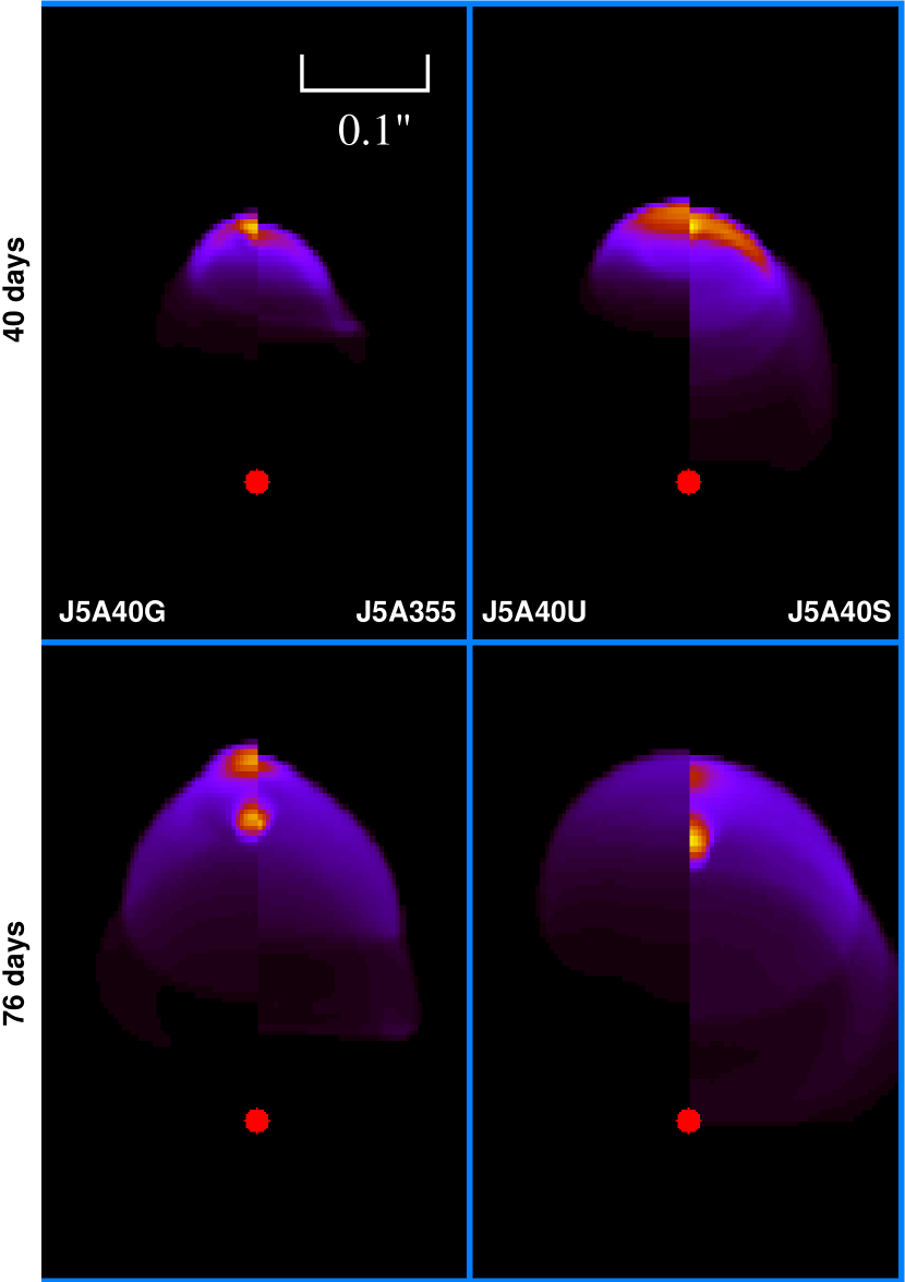
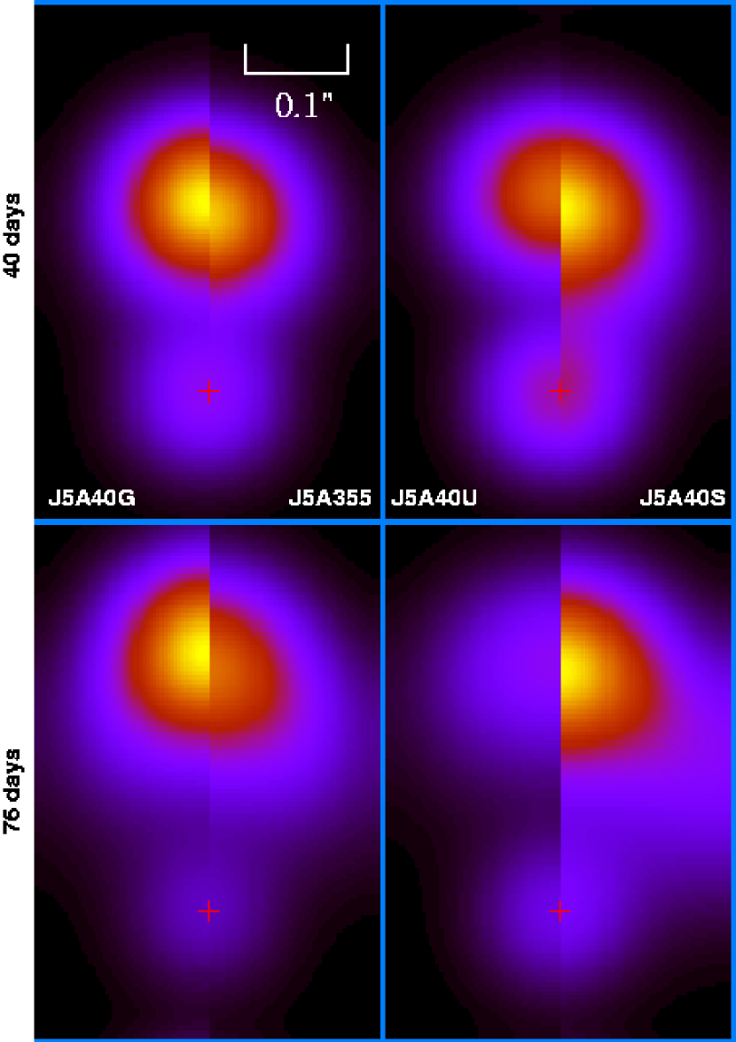
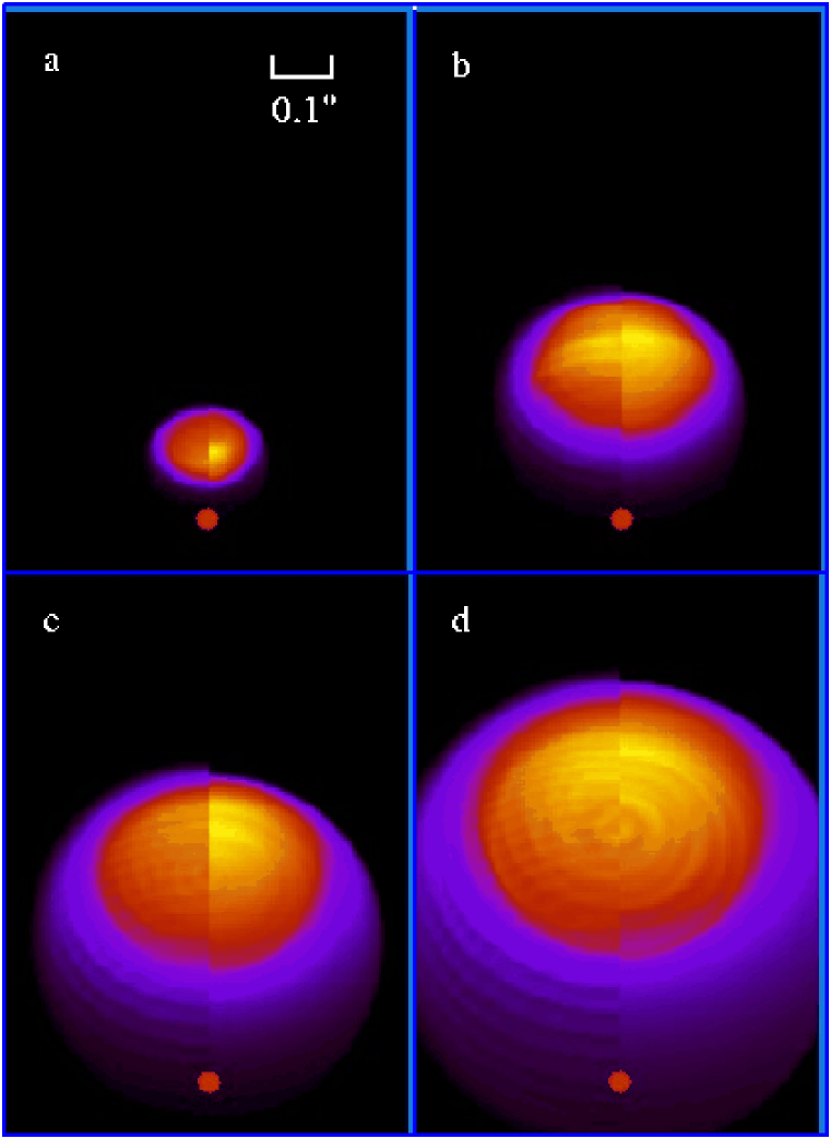
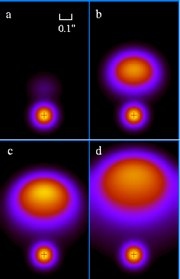
In order to compare the observational features of different models, it is useful to construct a synthetic, observer-eye-view flux map of the emission, as shown in Figure 7. These images show the position and shape of the Epoch II emission with respect to the SGR. Note that all of the non-uniform models exhibit a characteristic double brightspot at later time - the leading (top) spot corresponding to the external shock, while the trailing spot corresponds to the collision of the flow-focused ejecta (§2.3). Figure 8 shows the same data as Figure 7, but with the image convolved with a 50 mas standard deviation gaussian point spread function. This blurring is meant to simulate the limitation in observable resolution. At this resolution the double brightspots are blurred together, but a marginal distinction can be made between the Epoch I and II emission regions.

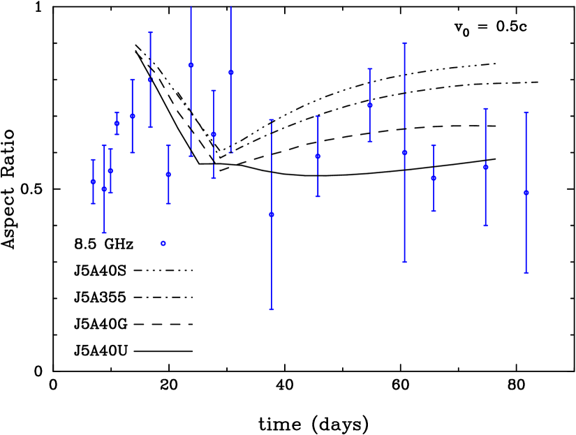
Taking the images of Figure 8 as being the most realistic, one can compare the predicted aspect ratio to that of observations as discussed in §3.3 and shown in Figure 9. The simulations exhibit a signature decrease-inflection-increase behavior which is the result of the emergence of the Epoch II flux component offset from the SGR (prompting a decrease in aspect ratio) until it surpasses the total flux from Epoch I (the inflection) and continues to gain dominance over it (the increase). The simulations show qualitative agreement with the data. Indeed, the hint of a decrease-inflection-increase behavior in the data, centered at around 30 days or so, is indicative of the veracity of the basic model of the emission being comprised of two independent epochs. The rapid decrease in aspect ratio at $\sim$ 30 days corresponds well with the rapid brightening of the flux curve and rapid motion of the centroid at this time (e.g. Figure 5), indicating that the emergence of the Epoch II flux component was swift, $\lesssim 10$ days.

4.2 Structured Jet Results

We find that the uniform jet model fails to produce the $t^{-1.1}$ decay slope observed for Epoch II, but instead decays more steeply. This is unexpected when one considers that the flux scaling for a jet with constant opening angle, $\theta_{0}$, and expanding with a Sedov-Taylor blastwave profile should go like

$$F\propto(r\theta_{0})^{2}rj^{\prime}\propto r^{3}{e^{\prime}}^{1.8}\propto r^{-2.4}\propto t^{-0.96}~{},$$ (38)

where $(r\theta_{0})^{2}r$ is the volume of radiating electrons with emissivity, $j^{\prime}\propto{e^{\prime}}^{(p+5)/4}$ (equations 31 & 32). For a strong shock the proper energy goes like $e^{\prime}\propto v^{2}$ and for a Sedov-Taylor solution, $v\propto r^{-3/2}$, while finally, $t\propto r/v\propto r^{5/2}$ (equation 4). Indeed we find these scalings to be good approximations of the simulations - except that $\theta_{0}$ is assumed to be constant. In reality, a rarefaction wave will propagate inward (i.e. poleward) from edge of the jet at the sound speed, $c_{s}$, thus reducing the effective radiating area. This rarefaction wave moves like $c_{s}\propto\sqrt{P/\rho}\propto\sqrt{e^{\prime}}\propto v$, where $P=(\Gamma-1)e^{\prime}$ and $\rho\propto\mathrm{constant}$ for strong shocks. So the jet’s radiating surface is roughly constant in time as it expands, and so the flux goes like

$$F\propto rj^{\prime}\propto r^{-4.4}\propto t^{-1.76}$$ (39)

which is consistent with the minimum (i.e. best fit) asymptotic slopes of uniform jets that we’ve simulated. Therefore, on theoretical and numerical grounds, the uniform jet does not satisfy the late time flux curve.

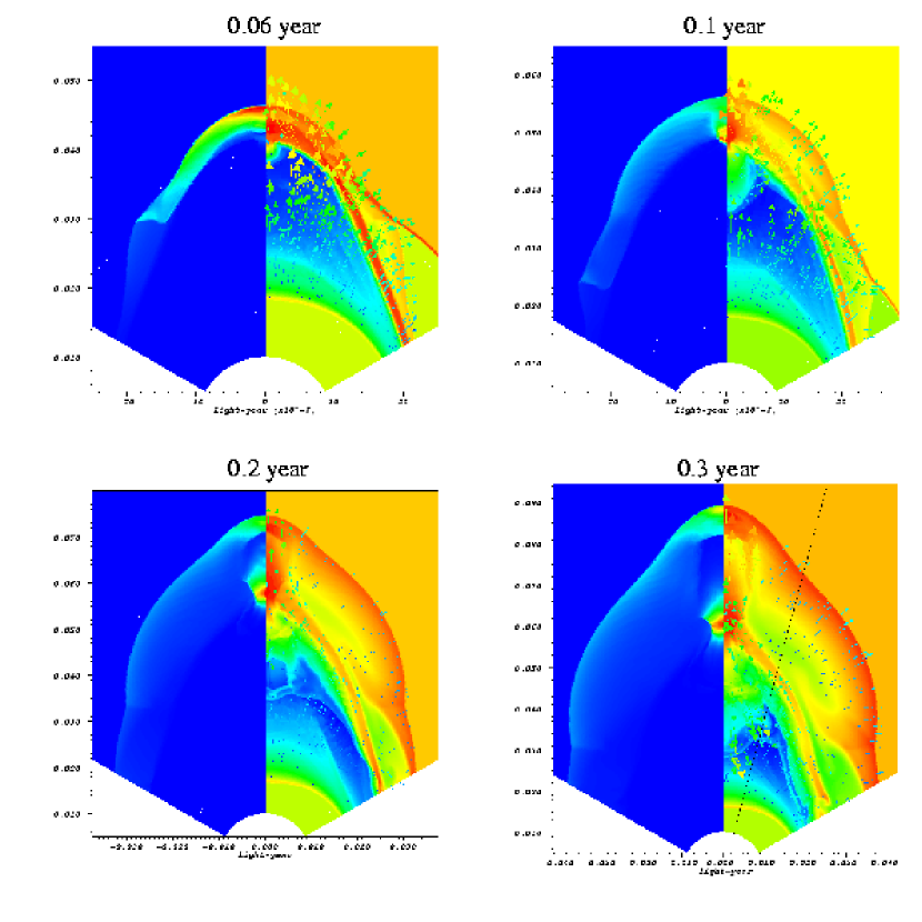
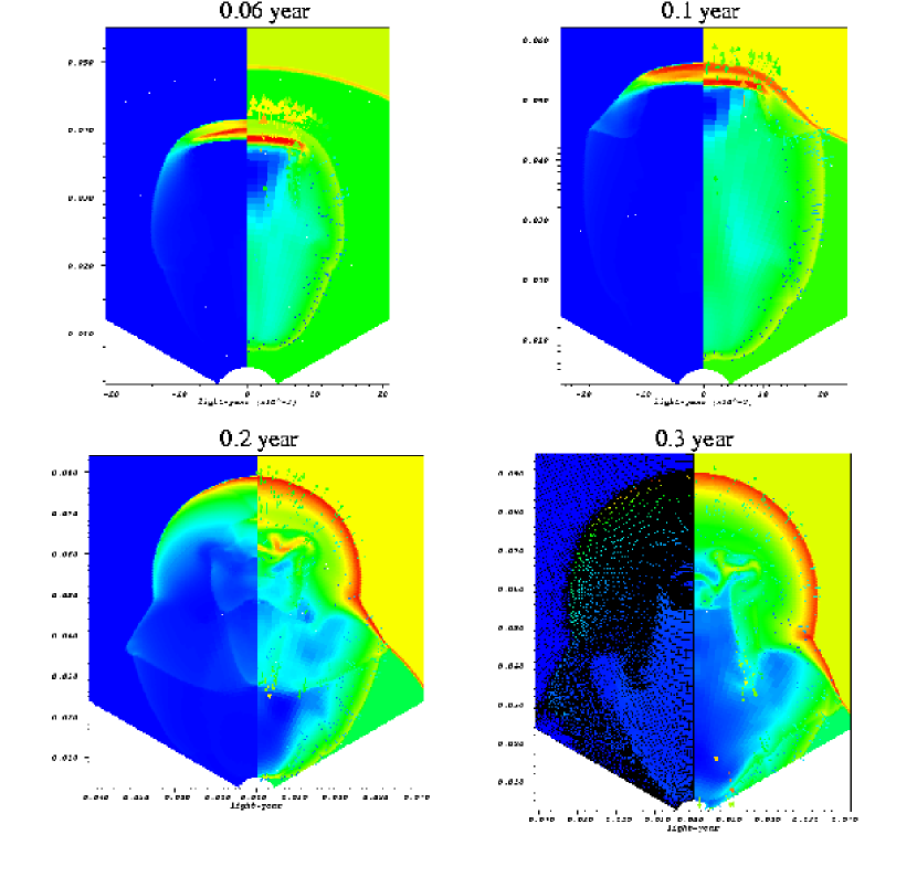
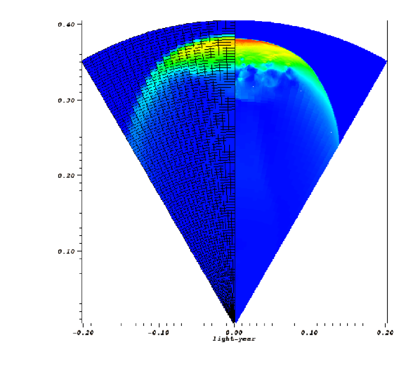
By contrast, both the structured and gaussian jets can be made to satisfy the $t^{-1.1}$ decay slope. The reason is a phenomenon we call “flow focusing”, which we find to be quite prevalent in models for which the velocity decreases with angle from the jet axis. The basic mechanism is as follows: If the jet is given some initial velocity variation $v(\theta)$ decreasing with angle, the ejecta front will distort as the material in the jet core begins to lead that in the wings. Thus, as the ejecta drives a shock into the external medium, a reverse shock is also driven back into the ejecta which, due to its distortion, will have obliquity and thus impart a poleward velocity into the ejecta. A secondary collision then results as the shocked ejecta collides onto the jet axis. This second shock produces a region of high pressure behind the on-axis portion of the external, forward shock which, in turn, drives it outward. Thus the on-axis forward shock velocity will be sustained for longer than expected in a typical Sedov-Taylor blastwave, and thus can create slower observed flux decay rates. An example of the flow-focusing in model J5A355 is shown in Figures 10 and 11. One can see a characteristic bowling pin shape to the forward shock at late time due to the added pressure of the secondary shock of the ejecta colliding on axis. This simulation can be contrasted with that of uniform jet J5A40U in Figure 12, where the lack of obliquity in the reverse shock does not prompt an on-axis secondary shock and so the evolution is much more akin to that of a Sedov-Taylor blastwave. The effect of flow-focusing on the lightcurve can be seen in Figure 6 where the the uniform jet shows much more rapid flux decay than the structured jets.

4.3 Doppler Brightening Results

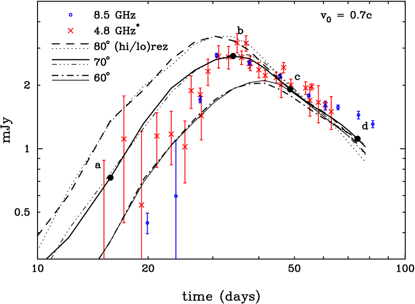
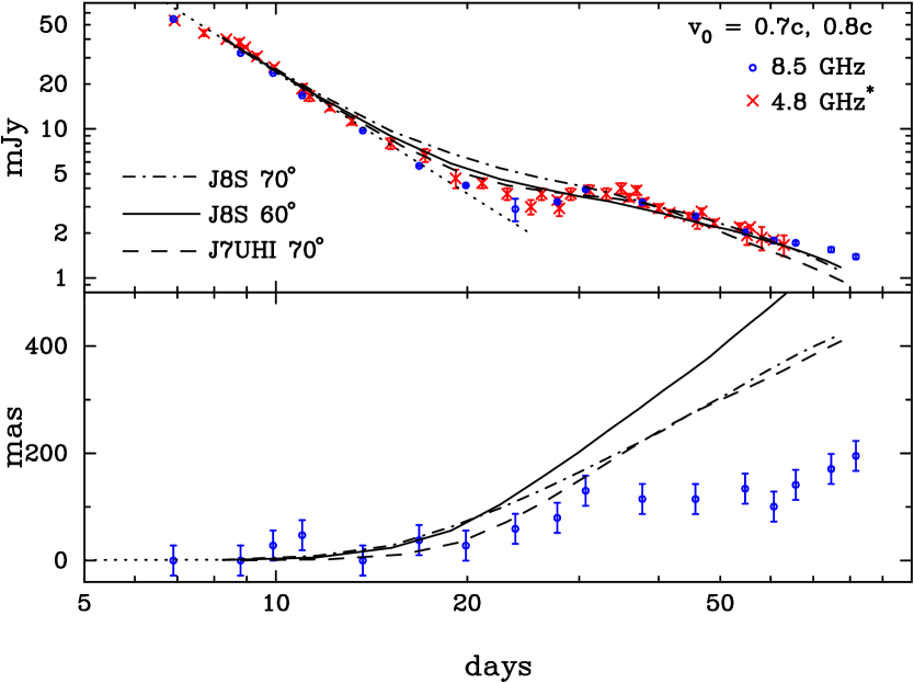
The last set of models we study here do not invoke a discontinuous increase in ISM density with a wall to prompt the observed rapid brightening of Epoch II. Instead, these models assume a sufficiently high Doppler factor (equation 21) to brighten and temporally compress the observed flux curve. In general, these models require higher velocities and inclination angles in order to achieve sufficient Doppler factors, as discussed in §2. In particular, we take the estimates from equations 8 and 11 and seek a uniform jet model with $v_{0}=0.7c$, $\theta_{i}=70^{\circ}$ and $\theta_{0}=12^{\circ}$. The results are shown in Figures 13 and 14. In general, these models have a much larger deceleration radius $\propto(E_{0}/n_{ext})^{1/3}$ (Table 1) than the collisional models. The qualitative agreement within errors is acceptable. However, one might ask if it is possible to improve the fit by creating a faster rise to peak and a slower decay therefrom. Unfortunately, these two goals are at odds with each other. Obtaining a steeper rise to peak requires a larger $v_{0}$ or $\theta_{i}$ in order to increase the Doppler factor and expedite the observed evolution. Such an adjustment would, in turn, also increase the decay slope, which is already steeper than the observation.

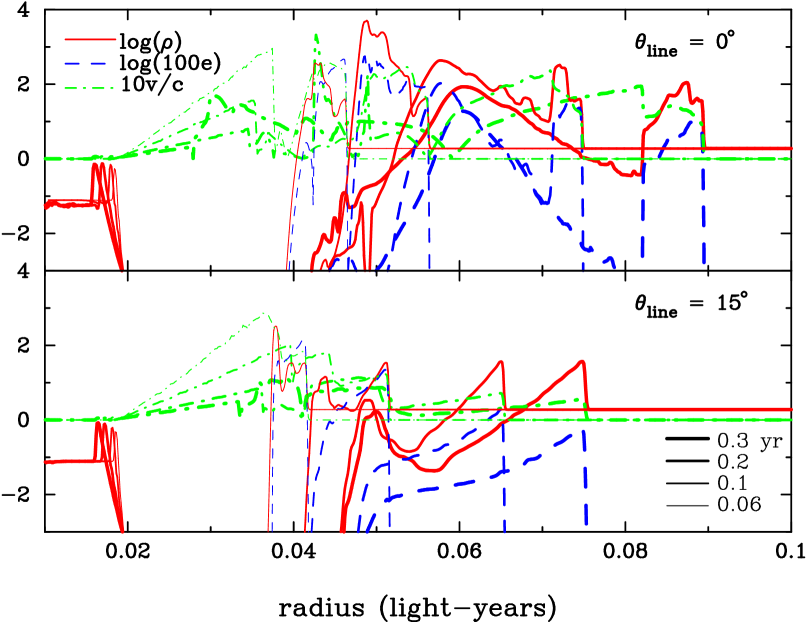
Figure 15 shows simulated flux maps similar to those of Figure 7. Because the external density, $n_{ext}$ is much lower than that of the previously discussed models ($<1$%), the forward shock travels further and becomes larger before decelerating. Figures 15 & 13 also demonstrate the level of numerical convergence of this model. Models J7UHI and J7ULO begin identically (requiring high resolution initially to resolve the problem features), but the latter progressively sheds its five layers of mesh refinement (due to an artificially high derefinement threshold in the proper mass density), having entirely deresolved the forward shock at the mid-time of the simulation, until it is entirely on the base mesh at the end of the simulation. The remarkably good agreement of the data from these two simulations is indicative of the stability of the results. Figure 16 compares the proper internal energy $e^{\prime}$, representative of shock heating, for both problems at the end of the run: 0.6 year. The problems exhibit excellent qualitative agreements.

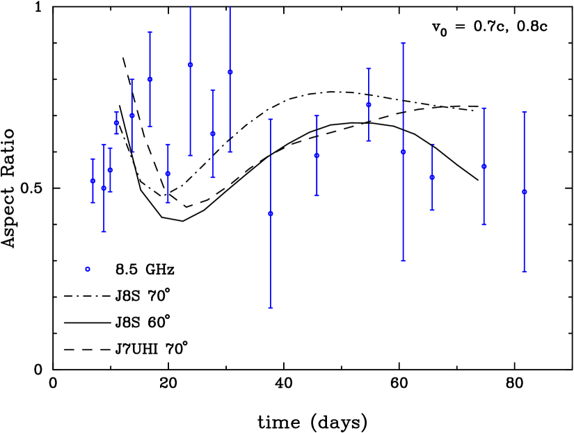
In Fig. 17, the images of Fig. 15 for model J7UHI are convolved with a 50 mas gaussian as was done in Figure 8. Once again, at this level of blurring, each epoch’s flux component should be resolved. The aspect ratio of this model is shown in Figure 18. The more gradual increase in flux from Epoch II in these uniform ISM models corresponds to a smoother minimum in aspect ratio (at $\sim 20$ days) than the sharp inflection seen in Figure 9.

Finally, we explore the possibility of a non-uniform jet plowing into the uniform, low-density ISM to see what effect flow-focusing observed in the earlier models might have in this case. The lightcurve for such a model, J8S (Table 1), is shown in Figure 19 for two inclination angles, $60^{\circ}$ and $70^{\circ}$, and the aspect ratio for these is shown in 18. Because of the relatively long distances traversed by the ejecta, a rather mild velocity variation was employed, $s=0.25$ (see equation 14). It is evident that J8S does not show improvement over J7UHI in the sharpness of the Epoch II peak, even though a higher initial velocity, $v_{0}=0.8c$, was used to attempt to increase the Doppler factor. However, it does exhibit a more gradual decay slope, $\propto t^{-1.1}$, compared to $\propto t^{-1.7}$ for J7UHI, which is consistent with the prediction of equation 39 and is more consistent with the observed slope.

5 Discussion

In this paper we have numerically modeled the radio nebula of the GF of SGR 1806-20 under the assumption that it was comprised of two independent flux components: Epoch I assumed to be centered on the SGR and to uniformly decay throughout the observational period; and Epoch II assumed to be due to the interaction with the ISM of the mass ejected from the SGR during the GF. In general we find that this two component model can satisfy all of the observations considered here: the lightcurve, the centroid position, and the nebula aspect ratio.

We have considered two models for how the Epoch II flux bump evolved. First, the collisional brightening model assumes that the rapid brightening of Epoch II is caused by the ejecta colliding with a wall or step in ISM density (§2.1). This model is very successful at producing the observed rapid flux brightening which precisely coincides with a rapid centroid motion (Fig. 5) and rapid decrease in aspect ratio (Fig. 9). Indeed, three distinct models of this class are presented, J5A355, J5A40S and J5A40G, all of which satisfy the data despite their varied inclination angles, jet structures, and total energies. Distinct by design, these models demonstrate some of the degeneracy in the observable characteristics. However, these models do constrain the initial ejecta velocity to be $v_{0}\sim 0.5c$. They also suggest that if there is a “wall” in the ISM, it must be several $\times 10^{16}$ cm from the SGR. If $v_{0}$ was much below this value, it becomes difficult to satisfy the centroid offset data (e.g. Figs. 3 &4), but if $v_{0}$ was much in excess of $0.5c$, implying a higher inclination angle to keep the centroid data consistent, one finds the flux to brighten more rapidly than is observed and a tendency for the late time flux decay rate to become steeper, due to Doppler contraction, than the $t^{-1.1}$ that is observed. Thus we believe these three models to trace out the locus of acceptable parameters for the collisional brightening paradigm.

It is interesting to note that the most successful models in this class had $n_{int}$ differing from $n_{ext}$ by only a factor of $\sim 4$. It may well be that models in which $n_{int}\approx n_{ext}$ can be made to work as well, therefore implying that, rather than reaching the terminus of a void, the Epoch II brightening might have occurred when the ejecta collided with a small cloud of material.

The second class of models we consider are Doppler brightened. In these models any collision with a density wall or discontinuity in the ISM is assumed to happen prior to any observations ($<7$ days) and so cannot be responsible for the rapid flux brightening of Epoch II. Therefore the brightening is only due to expansion of the shock forward of the ejecta as it plows into the ISM. Thus the only way to control the shock brightening is by Doppler contraction of the evolution as seen by an observer at high angle of inclination (§2.2). Thus these models require higher $v_{0}$ and $\theta_{i}$. The two models presented which best match the data are J7UHI and J8S. Both qualitatively match the data, but miss the finer features in Epoch II: the rapid flux brightening coupled with rapid centroid motion and aspect ratio decrease. To improve the fit in these respects, the initial ejecta velocity and inclination angle need to be higher than what was used here $v_{0}>0.8c$, $\theta_{i}>70^{\circ}$. Since increasing these parameters makes the final decay slope steeper, a structured jet morphology, as in model J8S, becomes more likely. Finally, one could appeal to spectral evolution effects such as a hardening spectral index $p$ (equation 32) to foster a more rapid brightening. So although these Doppler brightened models do not fit the data as well as the collision-brightened models (with their extra degrees of freedom associated with the ISM wall), they might be improved with added physics in future work.

A key difference between these two models is the scale of the external density $n_{ext}$. As can be seen in Table 1, the collisional brightening models J5A355, J5A40S and J5A40G have external densities greater than 100 times larger than those of the Doppler brightened models J7UHI and J8S, but all these models have a similar total energy, $E_{0}\sim 10^{46}$ ergs. Considering the scaling of eqn. 34, $n_{ext}\propto E_{0}$, an independent constraint on the external density might help discriminate between the two models. For instance Granot et al. (2006) place a lower bound, $n_{ext}\geq 10^{-2}$, which requires $n_{ext}$ and thus $E_{0}$ be scaled at least three times higher than quoted in Table 1. On the other hand, an upper bound on $n_{ext}$ would require $n_{ext}$ and thus $E_{0}$ to be scaled down for the collisional brightening models, which requires improved shock radiation efficiency (eqn. 35) which might become physically untenable.

Finally, in all of the models we discuss here we find that a non-uniform jet, with a velocity profile decreasing with angle from the jet axis, is required to fit the decay slope of Epoch II, $t^{-1.1}$. As discussed in §4.2, this is the result of “flow focusing” behind the external shock, which maintains the strength of this shock and thus extends the duration of emission. While some basic tuning was required (see Table 1) to fit the data, the general feature of flow focusing seems very generic and ubiquitous for non-uniform velocity distributions. To further explore and test this idea, it would be useful to have late time ($>80$ days) flux measurements to catenate onto those used here and compare with similarly extended simulations. It is very reasonable to imagine that jetted outflows generated by nature will be faster at the core than in the wings. Thus this effect might appear in other jetted phenomena such as gamma-ray bursts or jetted outflows from active galactic nuclei. It will be the subject of future work to explore other instances of this mechanism.

Figure 2: Flux curves of jet collision simulation J35A at four inclination angles, $\theta_{i}$, out of the view plane, toward the observer. These are compared with 8.5 GHz data (Taylor et al., 2005) and scaled 4.8 GHz data (Gelfand et al., 2005), each with the Epoch I flux component subtracted off. Inclination angle strongly affects the timing and brightness of observed flux. The best fit for this jet simulation is $\theta_{i}=55^{\circ}$.

Figure 3: Flux curves (top) and centroid position offsets in milliarcseconds (bottom) for simulation J35A seen at four inclination angles, $\theta_{i}$. Compare with Fig. 2 with the same data, but without the Epoch I flux component. Jet inclination $\theta_{i}=55^{\circ}$ most accurately matches the lightcurve. The flux centroid has zero offset from the SGR until the shock from the ejecta collision with the external medium brightens. Thus we see a rapid acceleration of the centroid position between 20 and 30 days. For inclination $\theta_{i}=55^{\circ}$, initial ejecta velocity $v_{0}=0.35c$ is seen not to be sufficient to produce the observed centroid offset, but the qualitative motion is evident.

Figure 4: Flux and centroid offset curves for three simulations, J377I25, J377I30, J377I35. All three match the data quite well, but are individually calibrated to match at individual angles of inclination, $\theta_{i}=25^{\circ},30^{\circ},35^{\circ}$ respectively. Model J377I35 is the same, except for $v_{0}$, as J35A in Fig. 3. Model J377I30 uses higher densities in the wall, $n_{wall}$ to produce the observed rapid rebrightening at a shallower inclination. Model J377I25 adds internal density, $n_{int}$, thus causing an earlier rise to the Epoch II flux, which better represents both the flux and centroid position data.

Figure 5: Flux and centroid offset curves for three simulations at $v_{0}=0.5c$: J5A355, J5A40S, J5A40G. These simulations are viewed at inclination angles, $\theta_{i}=-5^{\circ}$, $40^{\circ}$ and $40^{\circ}$ respectively. Each of these models show excellent agreement with the data, despite wide variations in the position of their external wall of material and jet structures. These models are typified by ejecta velocity, $0.5c$, which allows consistency with centroid offset data (bottom plot), a collision with an external wall initiating the rapid flux rebrightening, and a structured jet which enables flow focusing and thus reproduction of the late-time $t^{-1.1}$ flux decay law.

Figure 6: Flux curves for a range of models for $v_{0}=0.5c$. Model J5A40S shows good agreement with the data (see Fig. 5). Model J5A40U is a uniform jet calibrated to the same peak flux. The rapid flux decay of this model demonstrates the important role of flow focusing of structured jets in producing the observed $t^{-1.1}$ flux decay law at late time. Models J5A40SE2 and J5A40SE.5 compare the effect of doubling and halving, respectively, the total ejecta energy, $E_{0}$. Finally, for J5A40SEN2, total energy, $E_{0}$, and all external densities, $n_{ext}$, $n_{int}$, $n_{wall}$ have been doubled. The fact that the flux curve for J5A40SEN2 can be scaled to match that of J5A40S demonstrates a robust hydrodynamic scaling.

Figure 7: Simulated flux maps of four models from Figs. 5 & 6 at two times. For the three structured jets one can see the two bright spots characteristic of flow focusing, while the uniform jet, J4A40U, can be seen to fade rapidly. Each of the four frames is $0.08\times 0.12$ ly² in size and both halves of each frame are plotted on the same color scale.

Figure 8: Same data as the previous figure 7, but with the Epoch I (eqn. 1) flux component added at the position of the SGR (denoted by the red “+”) and the image is then convolved with 50 mas gaussian to simulate resolution limitations. Thus the total flux from one of these flux maps corresponds to the total flux in Fig. 5. One can see the rapidly fading Epoch I SGR flux component and that 50 mas resolution begins to differentiate the two flux components.

Figure 9: Aspect ratios are plotted for the simulated flux maps of the four models shown in Fig. 8. The simulated aspect ratio is defined in §3.3. This is plotted against the axial ratio of the ellipse fit by Taylor et al. (2005) to the observed emitting region. All simulations exhibit a decrease in aspect ratio as the Epoch II flux component increases, and an inflection and subsequent increase when the Epoch II flux exceeds that of Epoch I. Model J5A40U shows the most constant aspect ratio after 30 days because, as seen in Fig. 6, Epoch II decays rapidly in this model and thus stays comparable in magnitude to Epoch I. It is intriguing that the data tends to hint at the same decrease-inflection-increase evolution in aspect ratio as the simulations, indicative of two independent epochs.

Figure 10: Snapshots from simulation J5A355 at four times. On the left of each panel, the proper internal energy $e^{\prime}$ is shown. On the right half $\log(\rho)$ highlights structure and the coordinate velocity field $\vec{v}$ is superposed. The ejecta collides with external medium and its flow is focused toward the jet axis. This, in turn, creates a secondary hot-spot on axis that powers the forward shock, creating the characteristic bowling pin shape of the forward shock at late times. At time 0.3 year the 15^∘ lineout (see Fig. 11) is shown for reference.

Figure 11: Radial lineouts through simulation J5A355 along two angles of inclination, $\theta_{\mathrm{line}}$, from the polar axis. Proper density, energy and velocity are represented for the same four times as shown in Fig. 10. One can see the flow focusing of original ejecta material onto the jet axis, $\theta_{\mathrm{line}}=0^{\circ}$, at roughly a radius of 0.05 - 0.06 lt-yr, which then drives the center of the jet forward. The forward shock can be seen to progress outward more rapidly for $\theta_{\mathrm{line}}=0^{\circ}$ along a time sequence of radii (0.045, 0.055, 0.075, 0.09) lt-yr, compared with (0.041, 0.051, 0.065, 0.075) lt-yr for $\theta_{\mathrm{line}}=15^{\circ}$.

Figure 12: Same plots as in Fig. 10, but for the uniform jet model J5A40U. In contrast to Fig. 10, the uniform ejecta is not imparted with a poleward velocity component, and therefore does not exhibit flow focusing but instead generates a more spherical external shock. The left half of the final time panel shows the adaptive mesh zoning.

Figure 13: Flux curves of uniform jet expansion simulations J7UHI and J7ULO as seen from three different inclination angles, $\theta_{i}=80^{\circ},70^{\circ}$, and $60^{\circ}$. These models only differ in their spacial resolution; J7UHI uses 5 levels of mesh refinement on top of the base mesh, while J7ULO, after being started at high resolution to resolve the initial motion, was deresolved to the base mesh, and thus has zone size $2^{5}=32$ times larger than J7UHI. The fluxes J7UHI were multiplied by 90% (see Table 1) to best match the data, but otherwise the agreement of these two resolutions is remarkable. As per the discussion in §2, the case in which $v_{0}=0.7c$ and $\theta_{i}=70^{\circ}$ basically satisfies the sharp peak of the Epoch II flux bump. However the decay slope of these simulations tends to be steeper than the data. The solid black dots designated a, b, c, d are points at which flux maps are displayed in Fig. 15.

Figure 14: Flux and centroid curves for model J7UHI seen at three inclination angles. While the $\theta_{i}=70^{\circ}$ simulation shows general agreement, note that the flux curves show a rounder, broader peak and steeper final decay than suggested in the data. The position of the centroid is dominated by the Epoch II component and is quite sensitive to inclination angle.

Figure 15: Simulated flux maps of the evolution of the radio nebula at the four times alphabetically indicated in Fig. 13. Here the left half of each $0.16\times 0.22\mathrm{ly}^{2}$ panel is from simulation J7ULO, while the right half is from J7UHI. The dot at the lower center of each panel indicates the position of the SGR. Both halves use the same intensity scale and exhibit close qualitative agreement despite their large difference in resolution. The low-resolution (left) simulation shows two sets of discrete concentric bands centered on the jet and the SGR, indicating its limitation in spatial and thus temporal resolution, respectively. As shocks bounce between the ejected mass shell and the forward shock, their transient flux is evident as broad bands concentric on the SGR; a most obvious example of which is seen in panel b).

Figure 16: A comparison of proper energy densities for simulations J7UHI (right) and J7ULO (left) at their completion time: 0.6 year. They are plotted on the same color scale. One can see the external shock has driven upward and expanded from its initial position, $r_{0}=0.01$ light-year. Both simulations used the same base mesh, shown on the left for reference, but J7UHI allowed 5 levels of refinement on top of this mesh. The structure in the flow behind the shock, at radius $\sim 1/3$ ly, is due to Rayleigh-Taylor instabilities disrupting the original disk of ejected mass.

Figure 17: Model J7UHI for the same sequence of images as in Fig. 15, but with the Epoch I (eqn. 1) flux component added at the position of the SGR (denoted by the red “+”) and the image is then convolved with 50 mas gaussian to simulate resolution limitations. The panel dimensions, $0.16\times 0.25\mathrm{ly}^{2}$, are slightly enlarged from those of Fig. 15 to accommodate the blurring.

Figure 18: Aspect ratios for higher velocity simulations show the same qualitative behavior as those in Fig. 9. Because these models exhibit a more gradual brightening of Epoch II (Fig. 13), the aspect ratio decreases earlier and has a smoother inflection before increasing.

Figure 19: Flux and centroid curves for model J8S seen at two inclination angles $60^{\circ}$ and $70^{\circ}$. J7UHI is shown at $70^{\circ}$, as shown in Fig. 14. Note that, while none of these simulations match the data during the flux rise of Epoch II, $\sim 20-30$ days, the structured model J8S gives a final flux decay slope that is more consistent with the observed $t^{-1.1}$.

Table 1: Table of simulations.

Name	$v_{0}/c$	$\theta_{0}$	jet (s)	$M_{0}$	$E_{0}$	$\mathcal{E}_{N}$	$r_{0}$	$r_{wall}$	$n_{ext}$	$n_{int}$	$n_{wall}$	Figures
Collisional Brightening Model
J35A	0.35	$24^{\circ}$	P	3.56	3.26	1.15	2	3.15	1.0	$10^{-6}$	0.6	2-3
J377I25	0.377	$24^{\circ}$	P	3.08	2.77	1.05	2	3.15	1.0	0.26	6.0	4
J377I30	0.377	$24^{\circ}$	P	3.08	2.77	1.05	2	3.15	1.0	$10^{-6}$	6.0	4
J377I35	0.377	$24^{\circ}$	P	3.08	2.77	1.15	2	3.15	1.0	$10^{-6}$	0.6	4
J5A355	0.5	$24^{\circ}$	P	2.53	2.35	0.7	2	3.5	1.04	0.26	5.1	5,7-11
J5A40S	0.5	$24^{\circ}$	P (0.5)	1.56	1.5	0.95	1	4.9	0.53	0.1	1.25	5-9
J5A40U	0.5	$12^{\circ}$	U	0.2	0.21	0.95	1	4.9	0.53	0.1	1.25	6-9,12
J5A40G	0.5	$15^{\circ}$	G (0.75)	1.09	1.03	1.15	1	4.9	0.83	0.21	1.3	5,7-9
J5A40SE2	0.5	$24^{\circ}$	P (0.5)	3.13	3.0	0.4	1	4.9	0.53	0.1	1.25	6
J5A40SE.5	0.5	$24^{\circ}$	P (0.5)	0.78	0.75	2.7	1	4.9	0.53	0.1	1.25	6
J5A40SEN2	0.5	$24^{\circ}$	P (0.5)	3.13	3.0	0.271	1	4.9	1.06	0.2	2.5	6
Doppler Brightening Model
J7UHI	0.7	$12^{\circ}$	U	0.6	0.76	0.9	1	1.1	0.003	$3\times 10^{-7}$	0.003	13-19
J7ULO	0.7	$12^{\circ}$	U	0.6	0.76	1.0	1	1.1	0.003	$3\times 10^{-7}$	0.003	13,15-16
J8S	0.8	$20^{\circ}$	P (0.25)	1.5	1.9	0.8	1	1.1	0.003	$3\times 10^{-7}$	0.003	18-19

References

- Anninos & Fragile (2003) Anninos, P. & Fragile, P. C. 2003, ApJS, 144, 243
- Anninos et al. (2005) Anninos, P., Fragile, P. C., & Salmonson, J. D. 2005, ApJ, 635, 723
- Cameron et al. (2005) Cameron, P. B., Chandra, P., Ray, A., Kulkarni, S. R., Frail, D. A., Wieringa, M. H., Nakar, E., Phinney, E. S., Miyazaki, A., Tsuboi, M., Okumura, S., Kawai, N., Menten, K. M., & Bertoldi, F. 2005, Nature, 434, 1112
- Chevalier (1998) Chevalier, R. A. 1998, ApJ, 499, 810
- Corbel & Eikenberry (2004) Corbel, S. & Eikenberry, S. S. 2004, A&A, 419, 191
- Duncan & Thompson (1992) Duncan, R. C. & Thompson, C. 1992, ApJ, 392, L9
- Figer et al. (2005) Figer, D. F., Najarro, F., Geballe, T. R., Blum, R. D., & Kudritzki, R. P. 2005, ApJ, 622, L49
- Gaensler et al. (2005) Gaensler, B. M., Kouveliotou, C., Gelfand, J. D., Taylor, G. B., Eichler, D., Wijers, R. A. M. J., Granot, J., Ramirez-Ruiz, E., Lyubarsky, Y. E., Hunstead, R. W., Campbell-Wilson, D., van der Horst, A. J., McLaughlin, M. A., Fender, R. P., Garrett, M. A., Newton-McGee, K. J., Palmer, D. M., Gehrels, N., & Woods, P. M. 2005, Nature, 434, 1104
- Gelfand et al. (2005) Gelfand, J. D., Lyubarsky, Y. E., Eichler, D., Gaensler, B. M., Taylor, G. B., Granot, J., Newton-McGee, K. J., Ramirez-Ruiz, E., Kouveliotou, C., & Wijers, R. A. M. J. 2005, ApJ, 634, L89
- Granot et al. (2006) Granot, J., Ramirez-Ruiz, E., Taylor, G. B., Eichler, D., et al. 2006, ApJ
- Hurley et al. (2005) Hurley, K., Boggs, S. E., Smith, D. M., Duncan, R. C., Lin, R., Zoglauer, A., Krucker, S., Hurford, G., Hudson, H., Wigger, C., Hajdas, W., Thompson, C., Mitrofanov, I., Sanin, A., Boynton, W., Fellows, C., von Kienlin, A., Lichti, G., Rau, A., & Cline, T. 2005, Nature, 434, 1098
- Kumar & Granot (2003) Kumar, P. & Granot, J. 2003, ApJ, 591, 1075
- Li & Chevalier (1999) Li, Z.-Y. & Chevalier, R. A. 1999, ApJ, 526, 716
- Rossi et al. (2002) Rossi, E., Lazzati, D., & Rees, M. J. 2002, MNRAS, 332, 945
- Rossi et al. (2004) Rossi, E. M., Lazzati, D., Salmonson, J. D., & Ghisellini, G. 2004, MNRAS, 354, 86
- Rybicki & Lightman (1979) Rybicki, G. B. & Lightman, A. P. 1979, Radiative Processes in Astrophysics (New York: Wiley)
- Salmonson (2003) Salmonson, J. D. 2003, ApJ, 592, 1002
- Salmonson & Galama (2002) Salmonson, J. D. & Galama, T. J. 2002, ApJ, 569, 682
- Taylor et al. (2005) Taylor, G. B., Gelfand, J. D., Gaensler, B. M., Granot, J., Kouveliotou, C., Fender, R. P., Ramirez-Ruiz, E., Eichler, D., Lyubarsky, Y. E., Garrett, M., & Wijers, R. A. M. J. 2005, ApJ, 634, L93
- Wijers & Galama (1999) Wijers, R. A. M. J. & Galama, T. J. 1999, ApJ, 523, 177