Photometry with FORS at the ESO VLT

Abstract

ESO’s two FOcal Reducer and low dispersion Spectrographs (FORS) are the primary imaging cameras for the VLT. Since they are not direct-imaging cameras, the accuracy of photometry which can routinely be obtained is limited by significant sky concentration and other effects.

Photometric standard observations are routinely obtained by ESO, and nightly zero points are computed mainly for the purpose of monitoring the instrument performance. The accuracy of these zero points is about 10%.

Recently, we have started a program to investigate, if and how percent-level absolute photometric accuracy with FORS can be achieved. The main results of this project are presented in this paper. We first discuss the quality of the flatfields and how it can be improved. We then use data with improved flat-fielding to investigate the usefulness of for FORS calibration and the accuracy which can be achieved.

The main findings of the FORS Absolute Photometry Project program are as follows. There are significant differences between the sky flats and the true photometric response of the instrument which partially depend on the rotator angle. A second order correction to the sky flat significantly improves the relative photometry within the field. Percent level photometric accuracy can be achieved with FORS1. To achieve this accuracy, observers need to invest some of the assigned science time for imaging of photometric standard fields in addition to the routine nightly photometric calibration.

European Southern Observatory
Karl-Schwarzschild-Strasse 2
85748 Garching bei München,Germany

1. Introduction

ESO operates two version of the FOcal Reducer and low dispersion Spectrograph (FORS, Appenzeller et al. 1998), FORS 1 and FORS 2. Routine nightly photometric calibration observations for the FORS and other ESO imaging cameras aim to provide photometric accuracy of about 5 to 10%. The primary purpose of these observations is to monitor instrument performance. In addition, they often are used to calibrate science observations which do not require highly accurate photometry. The ESO FORS Absolute Photometry Project (FAP) recently used FORS1 to investigate the accuracy of photometry with that camera with the goal to establish procedures and advice observers with percent level photometric calibration needs. The specific goal of FAP was to demonstrate the feasibility of 3% photometry. This report describes the methods and results of FAP.

2. FORS Flats

The quality of the flatfields determines to a large extend the accuracy of relative photometry. For FORS, twilight sky flats are used almost exclusively. twilight flats are routinely taken at the start and end of the night, usually in groups of 4 frames. One area of concern in any is the presence of large scale features in the flatfields which do not correspond to variations in the sensitivity as a function of position on the detector. If for example illumination gradients are present, they will be propagated into the science images and the resulting photometry will be affected by position-dependent systematic errors.

Such gradients in flatfields are often introduced by the illumination source, in the case of FORS flats the twilight sky. Gradients or other flatfield artifacts can also be introduced by the instrument, e.g. through scattered light. Both issues are examined in this section.

2.1. Sky Gradients

During twilight, the sky is known to show illumination gradients, which change with time and the position of the Sun relative to the pointing of the telescope. Under conditions which are typical for FORS sky flats, the measured gradients can range from 2 to 5% per degree (Chromey & Hasselbacher 1996). For the field of view (FOV) of FORS (6^′.8$\times$6^′.8), this translates into natural gradients that range from 0.2 to 0.5%. On these small spatial scales, the illumination pattern is expected to be well approximated by an inclined plane, whose maximum gradient direction and intensity changes with the position of the Sun relative to the imaged sky. In principle, such sky gradients can be removed from individual flats before stacking them (Chromey & Hasselbacher 1996).

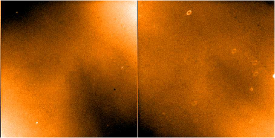
Figure 1.: Comparison between two $R$ flats taken on July 14, 2005 on 10:59:19.530 (left) and 22:43:32.037 (right). The images are flatfields divided by the mean of all flatfields for that night. The intensity scale range is 3%.

The structure in observed FORS flatfields reaches peak-to-peak values of more than 3%, i.e. an order of magnitude higher than typical twilight sky gradients. The structure in flat fields taken in consecutive or even the same night sometimes differs substantially. This is illustrated in Fig. 1, were we compare two FORS1 $R$ band flats taken about 12 hours apart. These changing structures, which dominate over the natural twilight sky gradients, make it difficult to judge whether such gradients are present in any given observed flatfield.

2.2. Instrumental features

In order to investigate the structure and amplitude of FORS1 intrinsic flatfield more systematically, we have retrieved from the ESO Archive all obtained between January 1, 2005 and September 30, 2005 in the $UBVRI$ passbands . The total number of images taken with standard resolution, 4-port read-out and high gain setting is 1083 ($U$: 148, $B$: 208, $V$: 226, $R$: 261, $I$: 240).

Each individual image was then bias-corrected using the pre-scan region only. We then computed the mean of the flatfields for each filter, and divided each individual frame by this mean. This removed the stable part of the flatfields such as the difference between the four quadrants and other large scale features. Finally, to allow quick visual inspection, we produced movies where each frame is an individual sky flat. Inspection of such movies revealed that the structure in the flatfields consists of a temporally constant pattern superimposed on large scale fluctuations which rapidly change in time. The contrast of the constant pattern is higher in bluer bands. We also found a correlation of some of the patterns with the adaptor rotator angle. FORS1 is mounted on an adapter rotator which compensates for the sky field rotation inherent to the VLT alt-azimuth mounting. Part of the structure in the flat field seems to rotate rigidly with the angle of the rotator. This is illustrated in in Fig. 2. This pattern in the flatfield must be external to FORS1 and might be due to reflections and/or asymmetric vignetting within the telescope or the adapter itself.

We extracted a high signal-to-noise version of the rotating structure in the following manner. First, we counter-rotated all $B$ images by an amount equal to the rotator angle reported in their FITS header. We then computed the median of the rotated flatfields. The resulting median image is shown in Fig. 2. If there were no correlation between the structure in the flatfields and the rotator angle, then the structure of the individual flatfields should average out and the median would be smooth and flat. Instead, the opposite can be seen can be seen in Fig. 2. A finger-like pattern, which is already visible in the individual flats shown in Fig. 2, stands out with increased signal-to-noise. It is therefore clear that this feature rotates. The peak-to-peak amplitude of the pattern is about 1%. Inspection of individual images in the stack shows that the amplitude varies substantially among the individual flatfields.

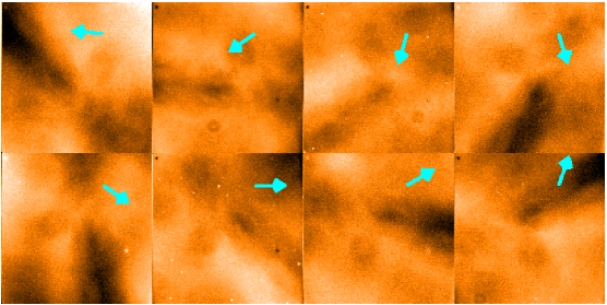
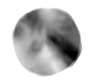
Figure 2.: Top: A sequence of $B$ FORS1 sky-flats. The rotator adapter angles ($-105^{\circ},-73^{\circ},-35^{\circ},0^{\circ},+30^{\circ}$, and +$70^{\circ}$) are indicated by a blue arrow in the upper right corner. Bottom: Stack of rotated $B$-band sky flats. Each image was rotated by the negative of the adaptor rotator angle

The existence of such a pattern imposes a limit on the accuracy of relative photometry reachable with FORS. If the feature is due to a rotation of the sensitivity pattern imprinted on all science frames, one would need to carefully match the rotator angle of the flatfield to those of each science frame. If, however, this feature is an additive component to the flat, removing it from the flatfield would improve the photometric accuracy of all flatfielded science data. One possible procedure to remove the rotating feature is to combine a large number of flatfield images taken with different rotator angles. If all angles are represented with the same weight, any rotating structure should smooth out. We tested this procedure with the $R$ band flatfields. In each rotator angle bin of $10^{\circ}$, we selected the same number of flatfields. We then computed the median of those flats. The result is shown in Fig. 3. The remaining structure in this combined flat is much more rotationally symmetric than the one in individual frames. There appears to be a small central light concentration.

Both, the rotating features shown in Fig. 2 and the illumination pattern shown in Fig. 3 appear to be stable in time, at least within the 9 month explored by this investigation. However, it should be emphasised that not all the variations in the flatfields can be described by a simple rotation. For example, the difference between the two flatfields shown in Fig. 1 seems to be similar to a $90^{\circ}$ rotation, but the adapter rotator angle changed by only about $25^{\circ}$. In Sec. 4. we will therefore investigate how FORS1 flat fields can be further improved.

2.3. Impact on Photometry

The key finding of this Section is that relative gradients in individual twilight flats as routinely obtained each night differ from each other by as much as 5%. If such flatfields are applied to science data, the relative photometric accuracy is limited to about 5%. Even when controlled for rotator angle, flatfields differ from each other by an amount which questions the goal of the current project, i.e. relative photometric accuracy of better than 3%. A key question is whether these fluctuations reflect true differences in the end-to-end throughput of FORS1. In that case, relative and therefore absolute accuracy at the percent level simply cannot be obtained with FORS1. An alternative explanation is that the flatfields are flawed and do not represent the throughput of FORS1. In that case, the task is to find the true flatfield which should be applied to data so that photometric zero points are constant over the whole detector. In the following sections, we will use data from the FAP programme to test the quality of the flatfields constructed in this section, and compare it to the regular “master flats” produced by combining the routinely taken twilight flats for that night.

              

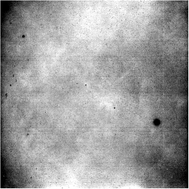
Figure 3.: Co-addition of a selected sample of 240 $R$ sky flats. Left: Image of the combined flatfield. The intensity scale range is 3%. Right: Traces along the central column (upper panel) and central row (lower panel).

3. FAP Data

3.1. Observations

Obtaining 3% photometric accuracy requires: 1) relative photometric calibration within each field; 2) absolute calibration of the extinction relation with slope and zero point; and 3) calibration of colour terms. Methods and data to obtain accurate relative photometry within the FORS1 field have been presented by Møller et al. in report II of the FSSWG project (Møller et al. 2005, hereafter FWII). For the current project, we aimed at an independent assessment of the relative photometric calibration to investigate whether the FWII results can be reproduced.

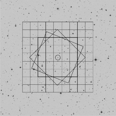
Figure 4.: Pointings on the Stetson Mark A field. The outline of the FORS1 frames are shown superimposed on the DSS field of that region. The well observed standard star , which is included in all frames is marked with a circle. Note the three different rotator angles used for the central field.

Our observations consisted of a $5\times 5$ grid of positions on the Stetson standard field Mark A (Stetson 2000) observed at low airmass. In addition, we observed one pointing on the grid of positions with two extra position angles. The pointings are shown in Fig. 4. All observations of that field were obtained at airmasses between 1 and 1.2.

In addition, we obtained data for the three standard fields , and observed at airmasses between 1.1 and 2.9. The FORS FOV is much smaller than the Stetson fields. We selected subregions of the standard fields which avoided bright stars. Unfortunately, for L113 a bright star was included in the observed field by mistake. This star saturated the CCD and led to bleeding, high background and bias offsets. For that reason, only a small fraction of the stars on the L113 field were useful, and 4 images had to be completely discarded.

All observations were carried out in a single photometric night on July 17, 2005.

3.2. Basic Data Reduction

Standard subtraction of overscan region and bias frames were performed using the IRAF “xccdred” package.

In order to compare the quality of flatfields, we used three different flatfields and applied them to the full set of data. They are:

MASTER FLAT:

Most reductions of FORS data use the “master flat” as produced by the FORS pipeline. This flat is basically the median of the flats taken for the night of observations. Below we simply refer to this flat as “”.

ILLUMINATION-CORRECTED FLAT:

As shown in the previous section, the large scale illumination of the flats is not stable and changes from exposure to exposure. We have therefore applied an illumination correction to the master flat by removing its large scale variation. We used the IRAF task “mkillumcor” for that purpose. This task heavily smooths the master flat and then subtracts this smooth version from the original master flat. The smoothing kernel used by mkillumcor is a boxcar function with fixed size in the central part of the image, and reduced size close to the edges. The minimum box size we used was 15 pixels, and the maximum 200 pixels. A 2.5$\sigma$ clipping was used to exclude deviant points from the computation of the smoothed image. Below we refer to this flat as “”.

ROTATION-CORRECTED FLAT:

Finally, as an experiment, we also used the mean of the archive flats shown in Fig. 3. As described in Sec. 2.2., the input flats were selected so that flats taken at any rotator angle are equally represented. We will refer to this flat as the “”.

3.3. Measurement of Magnitudes

Stars were identified and instrumental magnitudes were measured using . Based on the inspection of the growth curve, we computed aperture magnitudes with an aperture radius of 2 arcsec, and compared them with Sextractor’s “automag”. The difference between the two magnitudes was found to be independent of the magnitude of the stars. Because of its smaller statistical error, the analysis was done using the “automag”.

4. Zero Point Variation Across the FORS1 Detector

The doubt about the quality of the flatfields discussed in Sec. 2.1. and raised by the FWII report warrants taking a closer look at any variations of the magnitude zero point across the detector when using the master flat. The goal is to derive a correction to the used flatfield similar to the one proposed by FWII to improve the accuracy of the flatfields. In addition, we aim to find a quantitative estimate of the accuracy of the final adopted flatfield.

4.1. 25 Points of Light

The dithered observations were planned with the specific intent of placing one of the Stetson standard stars, namely Mark A-S873, on a grid of positions on the CCD (see Fig. 4). This approach is often nicknamed the “1000 points of light” approach, but we call it more modestly the “25 points of light”. The simplest and most direct way to investigate relative with such data is to plot the relative instrumental magnitudes of Mark A-S873 as a function of position. Such a plot is shown in in the left panel of Fig. 5. It can be seen that any relative photometric errors within the part of the detector sampled by our grid are on the order of 30 mmag or less. The sensitivity achieved with this analysis is insufficient to convincingly detect flatfield variations.

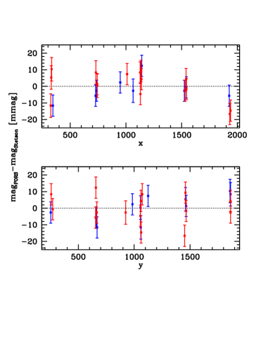
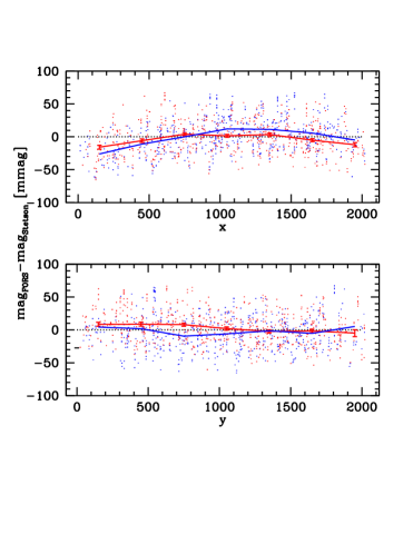
Figure 5.: Left: Data for Mark A-S873. The colour of the points in the upper panel indicates the $y$-coordinate of the star in each observation. For $y>1024$, points are red, and for $y<1024$, points are blue. Similarly, in the lower panel, red stands for $x>1024$, and blue for $x<1024$. Error bars are statistical errors. Right: Data for all Stetson stars in the Mark A field are plotted. Solid lines show the data binned in 100 pixel wide bins.

4.2. 1000 Points of Light

Better statistics than in Fig. 5 can be obtained by including all stars with magnitudes listed by Stetson. About 1000 magnitudes of Stetson stars have been measured from our data set. The right panel in Fig. 5 shows the difference between instrumental magnitudes and Stetson magnitudes as a function of position on the detector. No bandpass correction was applied. The scatter of individual points in this plot is larger than the scatter in Fig. 5 because of errors in the Stetson magnitudes and because differences between the FORS1 and Stetson’s effective filter shapes makes the zero point of stars depend on colour. This is more than compensated by the larger number of measurements. This larger data set clearly detects some deficiencies in the flatfield with total peak-to-peak error in relative photometry, within the inner part of the detectors, of about 30 mmag.

4.3. Many Points of Light

$f(x,y)$

The images of our data set contain many more stars suitable for photometry than the ones listed by Stetson. The large number of stars allows to simultaneously fit for relative zero points of each image, the relative magnitude of each star and zero point variations across the field. FWII describes a method to find such a solution from a set of measured magnitudes on a set of dithered images. The power of this approach comes from the much larger number of stars which can be used to improve the statistics compared to the previous approaches. By contrast, the number of free parameters (one for each star and observed field) increases only modestly.

Figure 6.: $R$-band flatfield correction frame.

FWII defined a flatfield correction factor $f(x,y)$, so that each measured magnitude of a star on any of the images can be written as

$$m_{\nu\mu}=M_{\nu}+z_{\mu}-f(x,y)$$ (1)

where $M_{\nu}$ is the magnitude of star $\nu$ within the chosen band, $m_{\nu\mu}$ is its instrumental magnitude measured on image $\mu$, and $z_{\mu}$ is the zero point of image $\mu$. Following FWII’s approach, we used a polynomial to model $f(x,y)$,

$$f(x,y)=\sum_{i=0}^{o}\sum_{j=0}^{o-i}p_{ij}x^{i}y^{j}.$$ (2)

The formalism to compute $f(x,y)$ is described in Appendix A

To estimate the uncertainties in the correction frame, we have carried out Monte-Carlo simulations in the following manner. First, we added normally distributed random errors to the measured magnitudes of each star. The standard deviation of the Gaussian was chosen to be identical to the error estimate in the actual measured magnitude. We created a total of 100 artificial data sets in this manner, and fitted $f(x,y)$ for each of them. We then computed the rms from all artificial data sets for each pixel.

Results

The resulting $f(x,y)$ flatfield correction is shown in Fig. 6. The peak-to-peak flat-fielding error at the position of the observed stars is about 30 mmag. The peak-to-peak flatfield correction over the whole field is about 50 mmag. However, over a large fraction of the detector, the corrections are smaller than 10 mmag and the rms over the whole frame excluding a strip 200 pixels wide along the edge is only about 4 mmag. Therefore, while flat-fielding problems on FORS1 might result in errors larger than our stated goal of 3% photometry for individual stars, statistically for random positions on the detector, the errors are much smaller. A different strategy for achieving accurate relative photometry with FORS1 is to concentrate on the centre part of the detector. For example, within the central $4\times 4\,$arcmin of the detector, roughly one third of the detector area, the difference between the minimum and the maximum of the correction factor is about 13 mmag, and the rms is 2 mmag.

Comparison with FWII

FWII used a similar procedure to the one used for the current work. In Fig. 7 and 8, we compare the results of our fit to the one in FWII. It can be seen that there is a good correlation between the two flatfield correction frames from data taken more about 15 month apart. The differences between the two determinations of $f(x,y)$ are similar in magnitude to the error estimates in $f(x,y)$. This suggests that there is a long term stable flatfield correction which can be applied to improve the photometric quality of images taken with FORS1 in the $R$-band.

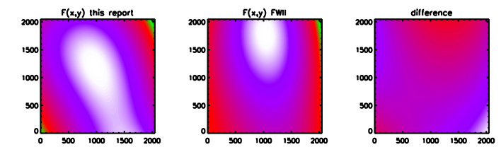
Figure 7.: Comparison between the flatfield correction frames derived in the current work and FWII. Left: $f(x,y)$ from FAP, center: from FWII, right: the difference. The colour scale in all three panels is identical.

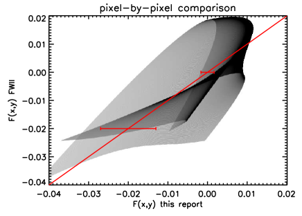
Figure 8.: Pixel-by-pixel comparison of $f(x,y)$ found by FWII and in the current project. The gray level indicates the number of pixels with the corresponding combination of values found by the two fits. The red line illustrates a one-to-one correspondence of the plotted values. The error bars are the minimum and maximum rms uncertainty for $f(x,y)$ estimated from the . The differences between the two frames are comparable to the uncertainty in the fits.

5. Improving the Master Flat

In Sec. 2.2. we have shown that a substantial component of the structure in the master flatfield rotates with the adaptor rotator. It is unlikely that any feature in the sensitivity map, i.e. the “true” flatfield, rotates. Therefore, it is most likely that the rotating feature is a defect in the master flats, e.g. caused by light scattered on some structure connected with the rotator. In this case, the derived flatfield correction should compensate for some of the structure found in the master flat. In the left panel of Fig. 9, we compare the master flat with the derived $f(x,y)$ on a pixel-to-pixel basis. We find that there is a significant correlation between the two frames. This suggests that the master flat could be improved simply by removing its large scale pattern.

This motivated us to create the illumination-corrected flat described in Sec. 3.2. We used the images flatfielded with this modified flat to re-measure magnitudes and re-derive the flatfield correction factor. A pixel-by-pixel comparison of the illumination-corrected master flat with the re-derived correction factor is shown in the right panel of Fig. 9. It can be seen that any correlation between flat and correction factor has successfully been removed, and that the peak-to-peak values of the correction factor have become smaller. This demonstrates that the master flat can be improved by this simple procedure. We also tested the same procedure on the $I$-band data, and on the FWII data and found similar results.

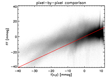
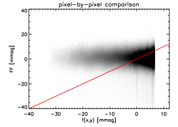
Figure 9.: Pixel-by-pixel comparisons of $f(x,y)$ with the flatfield (FF) used to process the images before fitting $f(x,y)$. Left: master flat versus derived $f(x,y)$, right: illumination-corrected flat versus $f(x,y)$.

The standard stars on the images can be used to verify that the flat-fielding is indeed improved by this procedure. For that purpose, we derived photometric solutions from the standard star measurements as described in Sec. 6., but without using the flatfield correction factor $f(x,y)$. The residuals as a function of detector position for the case of the regular master flat and that of the illumination-corrected flat are compared in Fig. 10. It can be seen that the illumination correction improves flatfield errors by as much as 50% in the centre of the field. However, it also shows that even using the illumination-corrected flats, significant flat-fielding errors remain and the flatfield correction procedure is still needed to reduce residual flatfield errors to values below 1%.

We have also tried the same procedure using the rotation-corrected flat shown in Fig. 3 but found no improvement over the standard master flat. We therefore will not use that flat in the further analysis.

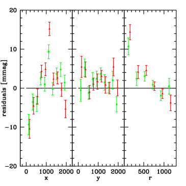
Figure 10.: Residuals from fit of photometric solution as a function of detector position. Left, centre and right panels show the mean residuals as a function of column $x$, row $y$ and distance from the detector centre $r$. The red points are derived using the regular master flat, and the green points used the illumination-corrected master flat. No flatfield correction $f(x,y)$ has been applied. Error bars are the errors of the means based on error estimates for the measured magnitudes and listed errors of the standard stars. Note that the mean of all the residuals is by construction zero. In the leftmost panel, the inner point contains fewer stars because it is based on a small area on the detector.

6. Absolute Photometry

6.1. Photometric Quality of Night

A crucial requirement for FAP was that observations were carried out under photometric conditions. The judgement whether a night on Paranal is photometric is done by the weather officer. This judgement is based on zero points derived from observations with the various imaging cameras, and inspection of the sky. Inspection of the sky is carried out by eye and with the help of MASCOT, a sky monitor which delivers optical images of the whole sky every three minutes. For FAP, the photometric quality of the night can be judged from the collected data. This might not be the case for science programmes which take significantly fewer calibration observations during a night. If such a programme requires photometric conditions, it is essential that the observer can judge the quality of the night objectively. This is of particular importance for service mode observations.

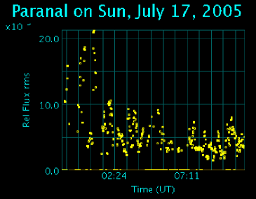
Figure 11.: The rms flux as measured by the ASM monitor.

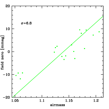
Figure 12.: Relative zero points of individual exposures of the Mark A field as a function of airmass as determined from the simultaneous fit of $f(x,y)$, relative magnitudes of stars and the exposure zero points. No standard magnitudes were used in deriving these data points. The solid line is the slope of the extinction correction as determined from the fit to Stetson magnitudes of stars. The rms of the deviations from this line is 6.8 mmag.

One of the tools to judge the quality of the night is the “VLT Astronomical Site Monitor” (ASM). Figure 11 shows the ASM flux fluctuations during the course of the night when the FAP observations were carried out. All FAP images were taken after UT 2:20 when the rms of the fluctuations was less that 10 mmag, and the mean rms fluctuation during that time was about 7 mmag. This rms from the ASM monitor can be compared to the flux fluctuations derived from the observations.

The procedure described in Sec. 4.2. yields the relative zero point for each image of the Mark A field. These zero points are already corrected for flat-fielding errors and each one of them is based on the weighted average of more than 1000 stars. The random errors of the relative zero points are therefore extremely small, about one mmag. Changes in the relative zero points are therefore a highly accurate measure of changes in the extinction between different images.

Figure 12 shows the relative magnitude zero points for the Mark A images as a function of airmass. The error estimate for each of the points based on the measurement errors is smaller than the point size. Also shown is the slope of the extinction curve derived from fields taken at higher airmasses, the details of this determination will be discussed in Sec. 6.3. It can be seen that the slope of the extinction curve is in excellent agreement with the variations of the zero point as a function of airmass. The rms scatter of the zero points around the extinction curve is 6.8 mmag. This experiment confirms the excellent photometric quality of the night completely independent of any standard star magnitudes.

The scatter of 6.8 mmag is a good measure of the fluctuations in the extinction within the 10 sec exposures. Its value is similar to the flux rms measured by the ASM monitor. It is tempting to conclude that the rms from the ASM can be used as a proxy for expected rms fluctuations of the zero point. Whether this is indeed the case warrants further investigation. For example, one area of concern is its sensitivity to seeing changes.

6.2. Photometric Solution

The method used to find the can easily be modified to find a photometric solution from the current data set. Instead of using an arbitrary zero point for each star and each field, the photometric zero point, colour terms and extinction coefficients are fitted. Specifically, we assumed that the instrumental magnitudes $r$ and the Stetson magnitudes $R$ and $I$ are related as

$$R-r=z+e\cdot x+a\cdot(R-I)+c\cdot(R-I)\cdot x$$ (3)

where $x$ is the airmass and $z$, $e$, $a$ and $c$ are parameters determined by the fitting. Those parameters were fitted simultaneously with the flat-fielding correction. The formalism is described in Appendix B.

We compared this solution to a separate fit of the correction frame $f(x,y)$ followed by a fit of the photometric solution. We found no differences in the results. All results in this section are based on the illumination-corrected flatfields and the additional application of the flat field correction derived from all detected stars.

Colour coefficients were fit using

$$r-i=c_{z}+c_{e}\cdot x+c_{a}\cdot(R-I)+c_{c}\cdot(R-I)\cdot x+c_{d}\cdot(R-I)^{2},$$ (4)

where $c_{z}$, $c_{e}$, $c_{a}$, $c_{c}$ and $c_{d}$ are the parameters of the fit.

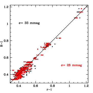
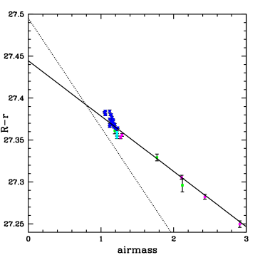
Figure 13.: Extinction and Colour solutions. Left: $R-I$ colours listed by Stetson versus the colours computed from the FAP data. Points in black use the colours based only on a fit of the zero point and slope of the colour correction, whereas red points use the full airmass and quadratic terms. Right: $R-r$ corrected for colour and colour-dependent extinction as a function of airmass. Each point is the weighted mean of all stars in one image. The colour of each point indicates the Stetson field from which the point was derived. The codes are: blue: Mark A, green: L 113, magenta: PG 1633 , cyan: L 92. The solid line is the fit to the data points and the extrapolation to zero airmass is shown to illustrate the magnitude zero point. For comparison, the photometric zero point and assumed extinction from the QC pipeline for that night is shown as a dotted line.

6.3. Results

Colour Solution

The linear component of the colour solution (Eq. 4) is shown in the left panel of Fig. 13. The scatter in the fit is about 28 mmag. This fit can be used to replace $R-I$ in Eq. (3) with its measured values. The uncertainty in the true colour adds less than 3 mmag to the random error of the final $R$ magnitude.

Extinction Solution

The resulting extinction solution is shown in right panel of Fig. 13. The ESO Quality Control (QC) group derives a photometric zero point assuming an extinction for each night. This QC zero point and extinction for that night are also shown in Fig. 13. There is a small offset between the normalisation of the QC extinction curve and the one derived here at airmass around 1.2. This offset might be due to slight differences in the normalisation of the flatfields, differences in the apertures used to measure magnitudes, and/or differences in the colour coefficients. However, the assumed extinction in the QC procedure introduces an additional error in the zero point which is much larger than the differences at airmass around 1.2. The extinction varies substantially from night to night, even when the nights are photometric. Therefore, zero points derived using a mean extinction depend on the airmass of the measured standard field and are not useful for photometry. The true photometric zero point above the atmosphere as derived from extrapolation of the extinction curves probably varied much more slowly than the night-to-night variations of the extinction. For this reason, when only a single photometric standard observation is available in a given night, the best practise is to derive the extinction coefficient for that night by assuming the zero point has not changed from the previous determination (cf. e.g. Harris 1981).

Figure 14.: Upper panels: Residuals as function of the estimated magnitude error. Lower panel: The $\sqrt{{\rm Var}}$ of the residuals as a function of magnitude error. The superimposed line corresponds to Var$=(7{\rm mmag})^{2}+\sigma_{M}^{2}$.

Residuals and Error Budget

Sextractor computes error estimates $\sigma_{s}$ for each measured magnitude. The error includes the contribution of the readout noise and Poisson noise, both for the pixels used to compute the stellar flux and for those used to estimate the local background. The error estimates ranged from 2 to 30 mmag. Stetson (2000) and Stetson (2006) list error estimates $\sigma_{st}$ for individual standard stars based on repeated observations in different nights. The error estimates for the stars used in this analysis range from 2 to 20 mmag. By comparing these error estimates to the residuals of the extinction solution, we can find an external estimate of the combined effect of all sources of errors not included in $\sigma_{s}$ and $\sigma_{st}$. For this purpose, we plotted the residuals from the extinction solution as a function of the error estimate $\sigma_{M}$ for each $R-r$. The plot is shown in the upper panel of Fig. 14. The error estimate $\sigma_{M}$ was computed as $\sigma_{M}=\sqrt{\sigma_{s}^{2}+\sigma_{st}^{2}}$. It can be seen that the scatter in the residuals for small estimated errors is less than 10 mmag and increases for larger $\sigma_{M}$. The lower panel of Fig. 14 shows the rms of the residuals binned by error estimates. A source of scatter in addition to the error estimate has to be assumed to account for the scatter residuals. Assuming this additional scatter $\sigma_{a}$ is independent of magnitude, the total scatter in the residuals $\sqrt{\rm VAR}$ can be modelled as

$${\rm VAR}^{2}={\sigma_{s}^{2}+\sigma_{st}^{2}+\sigma_{a}^{2}}$$ (5)

The lower panel of Fig. 14 shows that a value of $\sigma_{a}\approx 7\,$mmag is consistent with the residuals.

Sources for $\sigma_{a}$ include extinction fluctuations $\sigma_{e}$, colour transformation errors $\sigma_{c}$ and residual flat-fielding errors $\sigma_{ff}$. The total error estimate $\sigma_{t}$ for our magnitude measurements becomes therefore

$$\sigma_{t}=\sqrt{\sigma_{s}^{2}+\sigma_{a}^{2}}\\ =\sqrt{\sigma_{s}^{2}+\sigma_{e}^{2}+\sigma_{c}^{2}+\sigma_{ff}^{2}}\\$$ (6)

In Sec. 6.1. we found that $\sigma_{e}\approx 7\,$mmag, and in Sec. 6.2. we estimated that $\sigma_{c}\approx 3\,$mmag. Using 8 mmag as the upper limit for $\sigma_{a}$, we find from Eq. (6) an upper limit on residual flat-fielding and other sources of errors of about $3\,$mmag. We therefore conclude that extinction variations, statistical errors and errors in the standard magnitudes account for most of the residuals of our photometric solution.

6.4. How many Standard Field Observations are Necessary?

An important goal of FAP is to find a set of guidelines on how to achieve a photometric accuracy of 3% or less. The photometric zero point is obviously an important factor which determines the final accuracy of the magnitudes. The FAP observations contain a large number of standard stars on each individual image, and the number of calibration images is much bigger than the number realistically taken for the calibration of normal science observations. An important part of the photometric guidelines are the necessary minimum number of standard fields needed to achieve a certain photometric accuracy.

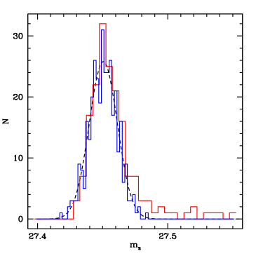
Figure 15.: Distributions of zero points determined from two (red histogram) and three (blue histogram) standard observations. The dashed line is a Gaussian with a $\sigma$ of 11 mmag.

FAP imaged four different Stetson fields. The magnitude and colour range, and the consistency of derived zero points seems to be similar for all fields (see e.g. Fig. 13). In addition, we searched for and did not find any evidence for different behaviour of the residuals as a function of position, magnitude or colour. Therefore, there is no evidence than anyone of the three fields Mark A, L92 or PG1633 is better suited for photometry than any other. As discussed in Sec 3.1., the particular region we used within the L113 field was not optimally chosen. Excluding the L133 field from the analysis in this section did not change any of the conclusions. For that reason, we do not distinguish between the different fields in the following discussion.

If a night is known to be photometric, e.g. by consulting the ASM, a minimum of 2 calibration fields at different airmasses are needed to find the extinction coefficient. The optimum strategy is that one of them is at as low an airmass as possible, while the other one is at the highest possible airmass. A realistic goal is to observe the low airmass field at an airmass less than 1.3, and the high airmass field at airmass above 2.

To estimate the errors in the zero points from sets of only two standard field observations, we re-computed the zero points from subsets of the FAP data. We used every combination of two standard fields which satisfy the above constraints on the airmasses. The distribution of the resulting zero points is shown in Fig. 15. The distribution has an almost Gaussian peak but also a long non-Gaussian tail. In about 10% of all cases, the errors on the resulting zero points is larger than 3%. We therefore conclude that observation of only two standard fields is insufficient to photometrically calibrate a night to sufficient accuracy.

We then repeated the experiment using 3 standard fields. In each case, only one of the three fields was chosen to be at airmass lower than 1.3, because the gain from additional low airmass fields was judged to be small. The resulting distribution of zero points is plotted in Fig. 15. Also shown is a Gaussian with the same mean, standard deviation and normalisation as the zero point distribution. It can be seen that the distribution resembles closely the Gaussian with a standard deviation of 11 mmag. In contrast to the previous experiment with only two standard fields, all zero point errors are less than 3%. This result strongly suggests that 3 photometric standard fields, chosen with the strategy outlined above, lead to an accuracy of about 11 mmag.

The $\chi^{2}$ per degree of freedom of the deviation between the Gaussian fit and the histogram in Fig. 15 based on count statistics is about 0.85. This means than the distribution of zero points when using 3 different standard fields very closely follows a Gaussian distribution. The error budget discussed in Sec. 6.3. implies that the dominant error on the mean magnitude of all stars in any of the standard fields are fluctuations in the extinction which affects all stars of an image in the same way. The only way to improve the magnitude zero point is therefore to increase the number of independent exposures. The fact that the distribution of the residuals shown in Fig. 15 is normal suggests that adding more stars will improve the accuracy of the zero point, and the final error in the zero point $\sigma_{Z}$ is

$$\sigma_{Z}\approx 11\,{\rm mmag}\cdot\sqrt{\frac{3}{n_{f}}}$$ (7)

where $n_{f}$ is the number of standard field observations. This formula should apply if the number of standard stars in each field is large enough so that

$$\sqrt{\frac{1}{\sum{\frac{1}{\sigma_{\rm STD}^{2}}}}}\ll 11\,{\rm mmag}$$ (8)

and the exposures sample the airmass between 1 and 2 uniformly. For a typical magnitude uncertainty $\sigma_{\rm STD}$ of 10 mmag, about 30 or more standard stars per field are needed to satisfy Eq. (8). This is one of the reasons to use the Stetson standard fields as opposed to fields with fewer known magnitudes. Unfortunately, the FAP data do not include a sufficient number of independent observation to test formula (7) for $n_{f}$ larger than 3.

The zero point error is a systematic additive error which affects all derived magnitudes in the same manner. The exact impact of such an error depends on the science application. In most cases, a programme with a stated goal to achieve 3 percent photometry requires that the systematic error is significantly less than 3%. The 10 mmag accuracy for the zero point might therefore not be sufficient for many photometric programmes even when they can accept much higher random errors. Eq. (7) can be used to guide observers. For example, the goal to achieve a photometric zero point better than 20 mmag with 99.7% confidence implies a $3\sigma$ error for the zero point of 20 mmag. Eq. (7) implies that eight standard fields are needed.

6.5. Three Percent Photometry

The above discussion shows that 3% photometry can be reached with FORS1 with moderate effort. For the purpose of this discussion, three percent photometry is defined as a total 1$\sigma$ error including both random errors on individual star and systematic errors due to zero point. With three calibration fields, the error in the zero point is 11 mmag (Sec. 6.4.). The maximum possible systematic error is 3 mmag (Sec. 6.3.). This leaves $\sqrt{30\,{\rm mmag}^{2}-11\,{\rm mmag}^{2}-3\,{\rm mmag}^{2}}=27.8\,$mmag for the possible random error in the magnitude of the science targets. A standard 1 hour Observing Block results in 50 minutes of open shutter exposure time. Using the ESO Exposure Time Calculator, we find that under standard conditions, the 3% goal can be reached down to a $R$ band magnitude of 24.3.

7. Conclusions

The main result of FAP is that it is possible to achieve 3% photometry with FORS1 with moderate effort. To achieve this accuracy, corrections to the standard master flats have to be applied, and a sufficient number of standard field observations have to be obtained. The Stetson fields seem to be well suited for that purpose. For service observations at ESO, observations of photometric standards in addition to the routine nightly calibration are charged to the science time. Observers therefore need to consider these calibration requirements during proposal writing and include them into the request for observing time. The results of Sec.6.4. can be used estimate the necessary observing time for calibration.

APPENDIX

Appendix A Formulae to fit $F(x,y)$ from stars without known magnitudes

In general, each measured magnitude on any of the images can be written as

$$m_{\nu\mu}=M_{\nu}+z_{\mu}-f(x,y)$$ (9)

where $M_{\nu}$ is the magnitude of star $\nu$ within the chosen band, $m_{\nu\mu}$ is its instrumental magnitude measured on image $\mu$, and $z_{\mu}$ is the zero point of image $\mu$. The quantity $f(x,y)$ is $F(x,y)$ expressed in magnitudes, i.e.

$$f(x,y)=-2.5\log F(x,y)$$ (10)

The specific model for $f(x,y)$ used for the fit to the current data set is a polynomial of order $o$,

$$f(x,y)=\sum_{i=0}^{o}\sum_{0}^{i}p_{ij}x^{i}y^{o-i}.$$ (11)

The magnitude for the $n+1$ different observed stars, $M_{\nu}$ where $\nu=0\ldots n$, and the zero points of the $m+1$ different images, $z_{\mu}$, $\mu=0\ldots m$, are further free parameters. Two of the three parameters $p_{0,0}$, $M_{0}$ and $z_{0}$ are redundant and can be arbitrarily fixed. Choosing $M_{0}=z_{0}=0$, the full set of equations 11 can be written as

$$\mathbf{A}\cdot\mathbf{p}=\mathbf{M}$$ (12)

where $\mathbf{p}$ and $\mathbf{M}$ are the vectors for the parameter and vector instrumental magnitudes,

$$\mathbf{p}=\begin{pmatrix}p_{0,0}\cr p_{1,0}\cr p_{0,1}\cr\vdots\cr p_{kl}\cr M_{1}\cr M_{2}\cr\vdots\cr M_{n}\cr z_{1}\cr z_{0}\cr\vdots\cr z_{m}\end{pmatrix},\ \ \mathbf{M}=\begin{pmatrix}m_{0,0}\cr m_{1,0}\cr m_{2,0}\cr\vdots\cr m_{n,0}\cr m_{0,1}\cr m_{1,1}\cr\vdots\cr m_{n,m}\end{pmatrix}$$ (13)

and the matrix $\mathbf{A}$ is

$$\begin{array}[]{lll}\mathbf{A}=\\ \tiny\begin{array}[]{rrcccccccccccccl}&&p_{0,0}&p_{1,0}&p_{0,1}&\cdots&p_{kl}&M_{1}&M_{2}&\cdots&M_{n}&z_{1}&z_{2}&\cdots&z_{m}&\cr 0&\hbox{\multirowsetup$\left.\vbox{\vrule height=180.0pt,width=0.0pt}\textrm{\hbox{}}\right($}&1&x_{0,0}&y_{0,0}&\cdots&x_{0,0}^{k}y_{0,0}^{l}&0&0&\cdots&0&0&0&\cdots&0&\hbox{\multirowsetup$\left)\vbox{\vrule height=180.0pt,width=0.0pt}\textrm{\hbox{}}\right.$}\cr 1&&1&x_{1,0}&y_{1,0}&\cdots&x_{1,0}^{k}y_{1,0}^{l}&1&0&\cdots&0&0&0&\cdots&0&\cr 2&&1&x_{2,0}&y_{2,0}&\cdots&x_{2,0}^{k}y_{2,0}^{l}&0&1&\cdots&0&0&0&\cdots&0&\cr\vdots&&&\vdots&&&&\vdots&&&&&\vdots\cr n&&1&x_{n,0}&y_{n,0}&\cdots&x_{n,1}^{k}y_{n,1}^{l}&0&0&\cdots&1&0&0&\cdots&0&\cr n+1&&1&x_{1,1}&y_{1,1}&\cdots&x_{1,1}^{k}y_{1,1}^{l}&0&0&\cdots&0&1&0&\cdots&0&\cr n+2&&1&x_{2,1}&y_{2,1}&\cdots&x_{2,1}^{k}y_{2,1}^{l}&1&0&\cdots&0&1&0&\cdots&0&\cr\vdots&&&\vdots&&&&\vdots&&&&&\vdots\cr n\times m&&1&x_{n,m}&y_{n,m}&\cdots&x_{n,m}^{k}y_{n,m}^{l}&0&0&\cdots&1&0&0&\cdots&1&\cr\end{array}\\ \end{array}$$ (14)

The parameters corresponding to each column are shown on the top of the matrix. Note that only a subset of all stars is contained in any single image, the labelling of the rows on the left side of the matrix is therefore not necessarily consecutive. The total number of free parameters to be determined $n_{p}$ is

$$n_{p}=n+m+\sum_{i=0}^{o}(i+1)=n+m+\frac{o^{2}+3o+2}{2}$$ (15)

whereas the number of equations is identical to the number of measured instrumental magnitudes. If the number of instrumental magnitudes per image is $>>2$, then Eq. (12) is an over-determined set of linear equations.

(SVD) can be used to find the unknown zero points, magnitudes and model parameters simultaneously in a least-square sense. SVD works by decomposing the matrix $\mathbf{A}$ into a square diagonal matrix $\mathbf{w}$ with positive or zero elements, and two orthogonal matrices $\mathbf{u}$ and $\mathbf{v}$,

$$\mathbf{A}=\mathbf{u}\cdot\mathbf{w}\cdot\mathbf{w^{t}}.$$ (16)

Then the least square solution for $\mathbf{M}$ can be found as

$$\mathbf{p}=\mathbf{v}\cdot\mathbf{w^{\prime}}\cdot\mathbf{u^{t}}\cdot\mathbf{M}$$ (17)

where $\mathbf{w^{\prime}}$ is a matrix which consists of a the inverse of a $n_{p}\times n_{p}$ submatrix of $\mathbf{w}$ and is set to zero elsewhere (see Press et al. 1992, for details).

One consideration for solving this set of equations is to assign proper weights to each equation. Eq. (12) still holds when each row in the matrix $\mathbf{A}$ as well as corresponding elements of the vector of instrumental magnitudes are multiplied by an arbitrary weight. We weighted each equation taking into account both the uncertainty in the measured instrumental magnitudes and the local density of stars.

The estimated uncertainty $\sigma_{\nu\mu}$ in the instrumental magnitude of the $\nu^{\it th}$ star in the $\mu^{\it th}$ field as given by Sextractor were used to compute a weight $w_{m}$,

$$w_{m}=\frac{1}{\sigma_{\nu\mu}^{2}}$$ (18)

A significant source of uncertainty in the fit of our model to the zero points is the difference between the true shape of $f(x,y)$ and that of the model polynomial. If an unweighted fit of a polynomial were used, more weight would be given to regions with high density of observed stars. This would introduce biases in the fit which can be avoided by adjusting the weights according to the local density of stars. Specifically, we have used the inverse of the local density of $w_{m}$ to compute a second weight $w_{\rho}$,

$$w_{\rho}=\frac{1}{\sum w_{m}}$$ (19)

where the sum in this equation is taken over all magnitude measurements in cells of $128\times 128$ pixels on the detector. The final weight used for each equation was

$$w_{t}=w_{\rho}\cdot w_{m}$$ (20)

Appendix B Formulae to fit $F(x,y)$ and extinction solution simultaneously

The formulae in Appendix A can easily be modified when the magnitudes of stars are known. The magnitude zero points for individual stars are replaced with the colour term, the zero points for individual images are replaced by the extinction terms, and the zero of the polynomial $p_{0,0}$ is replace by the constant magnitude zero point to find the parameters of Eq. (3).

The parameter vector $\mathbf{p}$ and $\mathbf{M}$ are in this case

$$\mathbf{p}=\begin{pmatrix}z\cr p_{1,0}\cr p_{0,1}\cr\vdots\cr p_{kl}\cr e\cr a\cr c\end{pmatrix}\rm{,\ \ \ }\mathbf{M}=\begin{pmatrix}M_{0}-m_{0,0}\cr M_{1}-m_{1,0}\cr M_{2}-m_{2,0}\cr\vdots\cr M_{n}-m_{n,0}\cr M_{0}-m_{0,1}\cr M_{1}-m_{1,1}\cr\vdots\cr M_{n}-m_{n,m}\end{pmatrix}$$ (21)

and the matrix $\mathbf{A}$ is

$$\begin{array}[]{lll}\mathbf{A}=\\ \begin{array}[]{rrcccccccccccccl}&&z&p_{1,0}&p_{0,1}&\cdots&p_{kl}&e&a&c\cr 0&\hbox{\multirowsetup$\left.\vbox{\vrule height=120.0pt,width=0.0pt}\textrm{\hbox{}}\right($}&1&x_{0,0}&y_{0,0}&\cdots&x_{0,0}^{k}y_{0,0}^{l}&X_{0}&c_{0}&X_{0}\times c_{0}&\hbox{\multirowsetup$\left)\vbox{\vrule height=120.0pt,width=0.0pt}\textrm{\hbox{}}\right.$}\cr 1&&1&x_{1,0}&y_{1,0}&\cdots&x_{1,0}^{k}y_{1,0}^{l}&X_{0}&c_{1}&X_{0}\times c_{1}&\cr 2&&1&x_{2,0}&y_{2,0}&\cdots&x_{2,0}^{k}y_{2,0}^{l}&X_{0}&c_{2}&X_{0}\times c_{2}&\cr\vdots&&&\vdots&&&&\vdots\cr n&&1&x_{n,0}&y_{n,0}&\cdots&x_{n,1}^{k}y_{n,1}^{l}&X_{1}&c_{n}&X_{1}\times c_{n}&\cr n+1&&1&x_{1,1}&y_{1,1}&\cdots&x_{1,1}^{k}y_{1,1}^{l}&X_{1}&c_{1}&X_{1}\times c_{1}&\cr n+2&&1&x_{2,1}&y_{2,1}&\cdots&x_{2,1}^{k}y_{2,1}^{l}&X_{1}&c_{2}&X_{1}\times c_{2}&\cr\vdots&&&\vdots&&&&\vdots\cr n\times m&&1&x_{n,m}&y_{n,m}&\cdots&x_{n,m}^{k}y_{n,m}^{l}&X_{m}&c_{n}&X_{m}\times c_{n}&\cr\end{array}\\ \end{array}$$ (22)

where $X_{\mu}$ is the airmass of the $\nu$th image, and $c_{\nu}$ is the R-I colour of the $\nu$th star. The least square solution for this set of linear equations can be found as above using Eq. 17.

Acknowledgments.

We thank Jason Spyromilio for granting technical time on FORS1 to carry out the FAP observations, David Silva and Sabine Moehler for useful discussions, and Jeremy Walsh for proof reading an earlier version of the FAP report.

References

- Appenzeller et al. (1998) Appenzeller, I. et al. 1998, The Messenger 94, 1
- Chromey & Hasselbacher (1996) Chromey, F.R. & Hasselbacher, D.A. 1996, PASP, 108, 944
- Harris (1981) Harris, W.E. 1981, PASP, 93, 507
- Møller et al. (2005) Møller, P., Järvinen, A., Rupprecht, G.,et al. 2005, “FORS: An assessment of obtainable photometric accuracy and outline of strategy for improvement (FORS IOT Secondary Standards Working Group)”, VLT-TRE-ESO-13100-3808 (FWII)
- Stetson (2000) Stetson, P.B. 2000, PASP, 112, 925
- Stetson (2006) Stetson, P.B. 2006, fields listed at http://cadcwww.dao.nrc.ca/cadcbin/wdbi.cgi/astrocat/stetson/query
- Press et al. (1992) Press, H., Tukolsky, S.A., Vetterling, W.T. and Flannely, B.P., 1995, Numerical Recipes in Fortran: The Art of Scientific Computing, Cambridge University Press, pp.51ff