How does the shape and thickness of the tachocline affect the distribution of the toroidal magnetic fields in the solar dynamo?

Flux-dominated solar dynamo models, which have demonstrated to be quite successful in reproducing most of the observed features of the large scale solar magnetic cycle, generally produce an inappropriate latitudinal distribution of the toroidal magnetic fields, showing fields of large magnitude in polar regions where the radial shear has a maximum amplitude. Employing a kinematic solar dynamo model, we here explore the contribution of both the radial and the latitudinal shear in the generation of the toroidal magnetic fields by varying the shape and the thickness of the solar tachocline. We also explore the effects of the diffusivity profile of the convective zone. Considering the shear term of the dynamo equation, $({\bf B_{p}}\cdot\nabla)\Omega$$=$$B_{r}{\partial\Omega/\partial r}+B_{\theta}/r\,\partial\Omega/\partial\theta$, we find that the latitudinal component is always dominant over the radial component at producing toroidal field amplification. These results are very sensitive to the adopted diffusivity profile, specially in the inner convection zone (which is caracterized by the diffusivity $\eta_{c}$ and the radius $r_{c}$ of transition between a weak and a strong turbulent region). A diagram of the toroidal field at a latitude of $60^{\circ}$ versus the diffusivity at the convection layer for different values of the tachocline width has revealed that these fields are mainly eliminated for tachoclines with width $d_{1}$$\gtrsim$$0.08R_{\odot}$ (for $\eta_{c}$$\simeq$$2\times 10^{9}$ $-$ $1\times 10^{10}$ cm² s^-1 and $r_{c}$$=$$0.715R_{\odot}$); or for $d_{1}$$\lesssim$$0.02R_{\odot}$ and almost any value of $\eta_{c}$ in the appropriate solar range. For intermediate values of $d_{1}$$\simeq$$0.04R_{\odot}$$-$$0.06R_{\odot}$, strong toroidal fields should survive at high latitudes in the butterfly diagram and those values are therefore not suitable. We have built butterfly diagrams for both a thin and a thick tachocline that best match the observations. We have also found that a prolate tachocline is able to reproduce solar-like butterfly diagrams depending on the choice of appropriate diffusivity profiles and tachocline width range.

1 Introduction

Over the last few years, with the increase of the computational power and the improvement in the observational techniques, there has been a substantial advance in the knowledge of our magnetic star. However there is still a considerable number of open questions regarding the magneto-hydrodynamic processes that govern the large scale solar magnetic phenomena, i.e., the 11-years sunspot cycle, the polarity inversions of the magnetic field, the phase lag between the toroidal and poloidal inversions, and the latitudinal distribution of the toroidal magnetic field. In the currently accepted scenario, the large scale solar magnetic cycle (LSSMC) is governed by a dynamo action that is the responsible for the transformation of a positively oriented poloidal magnetic field in a negatively oriented toroidal field, and the subsequent transformation of this one in another poloidal field but with the opposed polarity, and so on, until completing the cycle. The first stage of the process is the well known $\Omega$ effect: the poloidal field lines are dragged (“frozen in”), and amplified by the differential rotation of the fluid. From early results of the helioseismology, there has been a common agreement that this process takes place in the tachocline, a thin layer ($\leq 5\%$ of the solar radii) located at the base of the solar convection zone ($\sim 0.7R_{\odot}$) where the transition from a uniformly rotating regime of the radiative core to a differentially rotating regime in the convective envelope occurs. The strong radial shear (${\partial\Omega/\partial r}$) that exists in this region suggests that $\Omega$ acts mainly in the tachocline instead of in the entire convection zone.
The second stage of the process, conventionally called $\alpha$ effect from the early days of the Parker turbulent mean field dynamo, consists in to convert this belt of toroidal field in a new poloidal field with opposite polarity. This subject has been the center of intense discussions and debates and an excellent revision of both, the $\alpha$ effect mechanisms and the several dynamo models can be found in Charbonneau (2005) and references there in. In this work we assume an $\alpha$ effect as the result of the decay of active bipolar magnetic regions (BMR), as it was originally proposed by Babcock (1961) and followed by Leighton (1969). The fundamental ingredient in this mechanism is the emergence across the convective bulk of magnetic flux tubes due to the Parker-Rayleigh-Taylor instability in order to form sunspots or active BMRs at the surface, while the BMRs decay they migrate to the poles carrying with them the necessary magnetic flux to neutralize the remnant poloidal field and generate a new one. Magnetic reconnection between big loops of both hemispheres happens in this phase, as observed.

Magnetic flux tube simulations (D’Silva & Choudhuri 1993; Fan et al. 1993; Caligari et al. 1995, 1998; Fan & Fisher 1996; Fan 2004) have shown that magnetic fields between $5\times 10^{4}$ and $10^{5}$ G are able to erupt across the convection zone and emerge to the surface with the observed inclinations in the sunspots (joy’s law). A sub-adiabatic layer is necessary in order to store magnetic field up to this strength and once again the tachocline is the best place to allow this storage and amplification. The decay of the BMRs at the surface requires both, super-granular diffusion and meridional transport, for this reason the numerical models of the solar dynamo that work in the kinematic regime, that is, ignoring dynamical back-reaction of the magnetic field on the flux, include four fundamental ingredients: differential rotation, meridional circulation, diffusion terms and a source of poloidal field (the $\alpha$ term).

Recent kinematic models in the above scenario have been able to reproduce the majority of the LSSMC features, but have failed at producing a correct latitudinal distribution of the toroidal field, showing intense magnetic fluxes at higher latitudes and, consequently, sunspots close to the poles. Nandy & Choudhuri (2002) found a possible solution to this problem by allowing the meridional flow to penetrate below the tachocline. Under this hypothesis, the magnetic flux will be stored in a highly sub-adiabatic region and will emerge only at the desired latitudes. This assumption has given rise to a new controversy: how much of the meridional flow must penetrate below the tacholine? On one side, in a recent work Chatterjee et al. (2004), working under this hypothesis, have been able to reproduce the characteristics of the solar cycle in the two hemispheres, and also the observed parity rule (Hale’s law). On the other side, numerical simulations of a meridional flow penetrating in a sub-adiabatic medium (Gilman & Miesch 2004) have shown that the dynamical effects of the fluid alone, without including magnetic field, do not allow a penetration below $5\%$ of the tachocline and, in the case that the flow can penetrate in some way the radiative zone, the penetration would be reduced to about few kilometers only. In a recent report, Rüdiger et al. (2005) confirm this result arguing further that a meridional circulation confined within the convection zone alone would be able to produce an $\alpha\Omega$ dynamo. Another problem that arises when the penetration of the flow in the radiative zone is allowed is the excessive burning of light elements in such a hot zone. Numerical models of mixing, based on helioseismic measurements of the sound speed and density profiles, indicate a maximum extent of mixing of $5\%$ inside the tachocline (Brun et al. 2002). Also, Guerrero & Muñoz (2004) developed a hybrid model using the profile of meridional velocities of Nandy & Choudhuri (2002) and the $\alpha$-term of Dikpati & Charbonneau (1999) and found that a deep meridional flow solves only partially the problem of the distribution of the toroidal fields at the polar regions. Recently, Dikpati et al. (2004) have found an appropriate combination of parameters that are able to better reproduce the observations, however, until now there is no clear physical process that is able to explain why the sunspots appear only at lower latitudes.

In this work, we use a modified version of the numerical code developed by Guerrero & Muñoz (2004) introducing more detailed diffusivity and $\alpha$ profiles, as suggested by Dikpati et al. (2004), aiming to explore how the shape and thickness of the tachocline may influence the latitudinal distribution of the toroidal field. Although during the entire dynamo process there are several mechanisms that are still not understood, such as, the exact values and the variations of the magnetic diffusivity in the convective and radiative envelopes, and the return flow properties, the actual radial and latitudinal operation of the $\alpha$-effect, or the quantity of poloidal field that can be produced by the decay of the BMRs, for our propose here, we will consider profiles that are constrained by helioseismology observations and also by new results of simulations.

In section §2 we present the basic mathematical formalism of the solar dynamo mechanism and some details about the construction of the model (a complete description of the numerical tool is given in Guerrero & Muñoz (2004)); in §3, we present a detailed discussion of the assumed profiles and the set of parameters that allow for a best fit to the observations. The results of our analysis are described in §4; and finally in §5 we sketch our conclusions.

2 The model

The equation that describes the spatial and temporal evolution of the magnetic field in an ionized medium is the magnetic induction equation, which under the assumption of azimuthal symmetry can be divided in its poloidal and toroidal components, respectively:

$$\frac{\partial A}{\partial t}+\frac{1}{s}({\bf u}\cdot\nabla)(sA)=\eta\left(\nabla^{2}-\frac{1}{s^{2}}\right)A+S_{1}(r,\theta,B)\quad,$$ (1)

$$\frac{\partial B}{\partial t}+\frac{1}{r}\left[\frac{\partial}{\partial r}(ru_{r}B)+\frac{\partial}{\partial\theta}(u_{\theta}B)\right]=({\bf B_{p}}\cdot\nabla)\Omega$$ (2)

$$-\nabla\eta\times(\nabla\times B)+\eta\left(\nabla^{2}-\frac{1}{s^{2}}\right)B\quad,$$

where ${\bf B_{p}}$$=$$B_{r}+B_{\theta}$$=$$\nabla\times A$ is the poloidal field and $B$ the toroidal field, $\Omega$ is the angular velocity, ${\bf u}$$=$$u_{r}+u_{\theta}$ denotes the meridional components of the velocity field, $s$$=$$r\sin\theta$, $\eta$ is the magnetic diffusivity, and $S_{1}(r,\theta,B)$ is a source that describes the $\alpha$-effect in the Babcock-Leighton dynamo.

The above equations are solved in a 2-dimensional mesh of $128$ $\times$ $128$ grid points by using the ADI implicit method within the physical domain: $0.55R_{\odot}\leq r\leq R_{\odot}$, and $0^{\circ}$ (pole) $\leq\theta\leq 90^{\circ}$ (equator). The boundary conditions are as follows: $B$ and $A$ are set to zero in the pole and in the bottom radial boundary. At the top boundary we set a vacuum condition, so that, $B(R_{\odot},\theta)=0$ and $A(R_{\odot},\theta)$ is smoothly matched with a vacuum photosphere-corona, $\left(\nabla^{2}-\frac{1}{r^{2}\sin^{2}\theta}\right)A$$=$$0$. At the equator, we set the toroidal component, $B$$=$$0$, and a continuous boundary, $\frac{\partial A}{\partial\theta}$$=$$0$, for the poloidal field.

3 The dynamo ingredients

As discussed above, a kinematic solar dynamo model needs four fundamental ingredients: differential rotation, meridional circulation, magnetic diffusivity and a poloidal source term. The characteristics of these ingredients are in part constrained by helioseismology observations but there is some degree of freedom in the choice of the parameters that may reproduce better the LSSMC features. We assume the following profiles and parameters in order to generate a fiducial model able to reproduce the observed butterfly diagram.

3.1 Differential rotation

One of the goals of the helioseismology was the determination of an accurate profile for the angular velocity both at the surface and in deeper layers. The results revealed a radiative core that is rotating with uniform velocity. This changes to a convective bulk that is rotating differentially with a retrograde velocity with respect to the radiative interior at higher latitudes and a pro-grade velocity at lower latitudes. The interface between these two regimes is a thin layer called tachocline. An analytical profile of this differential rotation was introduced by MacGregor & Charbonneau (1997) and used for the first time in a Babcock-Leighton type dynamo by Dikpati & Charbonneau (1999). We employ here the same expression used by Dikpati & Charbonneau (1999):

$$\Omega(r,\theta)=\Omega_{c}+\frac{1}{2}\left[1+\mathrm{erf}\left(2\frac{r-R_{c}}{d_{1}}\right)\right](\Omega_{s}(\theta)-\Omega_{c})\quad,$$ (3)

where $\Omega_{c}/2\pi$$=$$432.8$ nHz is the uniform angular velocity of the radiative core, $\Omega_{s}(\theta)$$=$$\Omega_{eq}+a_{2}\cos^{2}\theta+a_{4}\cos^{4}\theta$ is the latitudinal differential rotation at the surface with $\Omega_{eq}/2\pi$$=$$460.7$ nHz being the angular velocity at the equator, $a_{2}/2\pi$$=$$-62.9$ nHz and $a_{4}/2\pi$$=$$-67.13$ nHz, erf$(x)$ is an error function that confines the radial shear to a tachocline located in $R_{c}$$=$$0.7R_{\odot}$ of thickness $d_{1}$. Figure 1 depicts the differential rotation profile in the solar interior for the core and convective layers.

Figure 1: Isorotation lines of the solar interior inferred from helioseismological observations. The dashed lines show the approximate thickness of the tachocline.

Until now there has been no consensus about the location and thickness of the tachocline (Corbard et al. 2001). Some observational works (Antia et al. 1998; Charbonneau et al. 1999), though of limited resolution, have found indications that this width may vary with latitude and suggested that the tachocline could have a prolate shape. We will show in section 4 how the change from a spherical to a prolate shape of the tachocline and its thickness influence the outputs of the model.

3.2 Meridional circulation

In the present stage of the observational techniques, there is a set of independent measurements of the meridional circulation that confirms a surface poleward flux of about $20$ m s^-1, which persists until a depth of $0.85R_{\odot}$ (Hathaway 1996; Hathaway et al. 1996; Latushko 1996; Snodgrass & Dailey 1996; Giles et al. 1997; Komm et al. 1993; Braun & Fan 1998). However, even helioseismology has been unsatisfactory to measure a deeper flow. Mass conservation predicts an equatorward return flow and a unique convection cell per meridional quadrant. Here, we use the same analytical prescription of Nandy & Choudhuri (2002) and Guerrero & Muñoz (2004), which was previously introduced by Dikpati & Choudhuri (1994), and Choudhuri et al. (1995):

$$\rho(r)\bf{u}=\nabla\times[\psi(r,\theta)e_{\phi}]\quad,$$ (4)

where $\psi$ is a stream function given by:

$$\psi r\sin\theta = (r-R_{p})\psi_{0}\sin\left[\frac{\pi(r-R_{p})}{(R_{\odot}-R_{p})}\right]$$

$$\times (1-e^{-\beta_{1}\theta^{\epsilon}})(1-e^{\beta_{2}(\theta-\pi/2)})$$

$$\times e^{[(r-ro)/\Gamma]^{2}}\quad,$$

and $\rho(r)$ is a density profile for an adiabatic sphere with a specific heat ratio $\gamma$$=$$5/3$ (polytropic index $m$$=$$1.5$), thus:

$$\rho(r)=C\left(\frac{R_{\odot}}{r}-0.95\right)^{m}\quad.$$ (6)

The value of $\psi_{0}$ and $C$ are chosen in such a way that the amplitude of the meridional velocity, $u_{\theta}$ at middle latitudes is $U_{0}$$=$$\psi_{0}/C$$=$$25$ m s^-1. The assumed value for the other five parameters are: $\beta_{1}$$=$$6.06\times 10^{9}$ cm^-1, $\beta_{2}$$=$$4.6\times 10^{9}$cm^-1, $\epsilon$$=$$2.0000001$, $r_{o}$$=$$(R_{\odot}-R_{min})/4.0$, and $\Gamma$$=$$3.47\times 10^{10}$ cm. $R_{min}$ is the radius of the bottom of the convective boundary,and $R_{p}$ is the radius of the penetration depth of the flow.

Figure 2: The adopted meridional circulation lines profile in this work. The dashed lines represent the tachocline with a constant thickness $d_{1}$$=$$0.05R_{\odot}$ in this case.

In a previous work, it has been shown that a deep meridional flow solves only partially the problem of the distribution of the toroidal magnetic field (Guerrero & Muñoz 2004). Besides, as stressed in §1, this assumption seems to need physical support and does not seem to be confirmed by numerical simulations either, so that, in the present analysis we will not adopt a deep meridional distribution (see however Nandy & Choudhuri (2002), and Chatterjee et al. (2004), for an alternative interpretation).

The dynamical shallow water model of Gilman & Miesch (2004) showed that it is impossible for the meridional flow to go below a few percent of the top for the solar tachocline. Recent calculations of Rüdiger et al. (2005) support this result arguing that a weak penetration is able to produce a flux dominated solar dynamo inside the solar convection zone, without the necessity of participation of the tachocline, however they did not consider the overshoot effect of plumes and jets that actually can penetrate inside the tachocline and even down in a thin fraction of a more sub-adiabatic medium (Rogers et al. 2006). In our calculations, we will assume a weak penetration inside the tachocline and, as the width of the tachocline is allowed to vary in this work, the percentage of penetration will be able to vary, as well, but we will consider a constant value for the penetration radius $R_{p}$$=$$0.69R_{\odot}$. Figure 2 shows the assumed meridional circulation profile.

3.3 Magnetic diffusivity

The radial dependence of the magnetic diffusivity is probably the most undetermined of the profiles of the solar interior. Diffusion must exist in the convective envelope due to the intense turbulence present, but besides the values of super-granular diffusion observed at the surface ($\eta_{S}\sim 10^{12}-10^{14}$ cm² s^-1), the depth dependence is uncertain and, in general, only approximate values are assumed for this quantity in the dynamo models. We will here follow Dikpati et al. (2004) and assume a weak turbulent diffusivity regime for the radiative interior, with $\eta_{r}$$=$$2.2\times 10^{8}$ cm² s^-1, a turbulent regime for the convective envelope, with $\eta_{c}$$=$$5\times 10^{9}$ cm² s^-1 above the tachocline, and a third region of super-granular diffusivity, from $r_{c1}$$=$$0.95R_{\odot}$ on, where $\eta_{S}$$=$$10^{12}$ cm² s^-1.

$$\eta(r)=\eta_{r}+\frac{\eta_{c}}{2}\left[1+erf\left(\frac{r-r_{c}}{d_{2}}\right)\right]+\frac{\eta_{S}}{2}\left[1+erf\left(\frac{r-r_{c1}}{d_{3}}\right)\right]\quad.$$ (7)

Different combinations of the parameters $d_{2}$, $d_{3}$, $r_{c}$, and $r_{c1}$ in the equation above can be considered (see, e.g., Dikpati et al. (2006)). The boundary between a weak and a strong turbulent regime is the location where an abrupt change in the temperature gradient occurs in helioseismic calibrations. We have presently considered $r_{c}$$=$$0.715R_{\odot}$ and $d_{2}$$=$$0.01R_{\odot}$ which are compatible with the values that have been obtained from helioseismic measurements, the first with a very high precision and the second as an upper limit (Basu 1997), and $r_{c1}$$=$$0.95R_{\odot}$, $d_{3}$$=$$0.01R_{\odot}$ (Dikpati et al. 2006) (see Figure 3). Our model is specially sensitive to the the diffusivity variation between the radiative core and the convective envelope. With the choice of the parameters above, we are considering a weak turbulent regime for the lower region of the tachocline and a turbulent regime for the upper part of it, with a sharp variation between them, in order to allow both storage of magnetic field and overshooting of material below the tachocline (see, however, §4.3 for a more detailed analysis of the dependence of the model with the parameters $\eta_{c}$ and $r_{c}$).

Figure 3: Adopted depth dependence of the magnetic diffusivity profile. Y axis is in log-scale and is normalized to the supergranular surface value ($10^{12}$ cm² s^-1).

3.4 The source of poloidal field (the $\alpha$ term)

From the Parker mean field dynamo theory days until now, the $\alpha$ source term of the poloidal field remains virtually undetermined. As a coupling factor between eqs. (1) and (2), the main function of this term is to generate poloidal field from pre-existent emergent magnetic flux tubes in the toroidal direction, and its form is oriented to resemble the Babcock-Leighton concept of formation of dipolar like field as the result of the decay of BMRs and the reconnection of loops from both hemispheres.

The magnetic flux tubes, at the base of the convection zone are amplified by the differential rotation until they reach a value such that the magnetic pressure begins to dominate over the gravitational pressure. Numerical simulations suggest a value of $10^{5}$ G. Then, they are lifted on the entire convection zone and twisted by the Coriolis force to form BMRs at the observed latitudes.

In order to allow this process to occur, we let the poloidal field at the surface ($r$$=$$R_{\odot}$) to be proportional to the toroidal field at the base of the solar convection zone ($r$$=$$R_{c}+d_{1}/2$), where $d_{1}$ is the thickness of the tachocline (see, e.g. Dikpati & Charbonneau (1999)). Since the toroidal field lines are mainly concentrated in a belt around the solar equator, following Dikpati et al. (2004), we consider the action of the Coriolis force also concentrated at lower latitudes, thus:

$$S_{1}(r,\theta,B) = \alpha_{0}\frac{1}{4}\left[1+\mathrm{erf}\left(\frac{r-r_{2}}{d_{2}}\right)\right]\left[1-\mathrm{erf}\left(\frac{r-r_{3}}{d_{3}}\right)\right]$$

$$\times \sin\theta\cos\theta\left[\frac{1}{1+e^{\gamma_{1}\left(\pi/4-\theta\right)}}\right]\left(1+\left[\frac{B(R_{c},\theta)}{B_{0}}\right]^{2}\right)^{-1}\quad,$$

where $r_{2}$$=$$0.95R_{\odot}$, $r_{3}$$=$$R_{\odot}$, $d_{2}$$=$$d_{3}$$=$$0.01R_{\odot}$, $\gamma_{1}$$=$$30$. The amplitude of the poloidal source is determined by $\alpha_{0}$ for which we assume a fixed value of $130$ cm s^-1. Figure 4 depicts the radial and latitudinal dependence of this profile.

Figure 4: Assumed radial and latitudinal profiles for the $\alpha$ effect mechanism. Radially, the $\alpha$ term is concentred close to the surface. Its latitudinal distribution corresponds to the belt where the sunspots appear.

The latitudinal dependence of $S_{1}$ is of great importance in the reproduction of the features of the solar cycle. We tested alternative possibilities reported in literature, i.e., profiles which are proportional to $\sin\theta\cos\theta$ (Dikpati & Charbonneau 1999), $\sin^{2}\theta\cos\theta$ (Küker et al. 2001), and $\cos\theta$ (Chatterjee et al. 2004) factors, but we found that the profile prescribed by eq. (3.4) is the one that better reproduces an observed butterfly diagram.

The last term on the RHS of eq. (3.4) is a quenching term limiting the growth of the poloidal field. Actually, this quenching should be given by the back reaction of the magnetic field on the velocity field, but the physical way by which the poloidal field stops growing is unknown. This form, which was also assumed previously by many authors, simply reproduces the fact that a toroidal field with a value larger than $B_{0}$$=$$10^{5}$ G would generate sunspot pairs with tilts which is in disagreement with the joy’s law (D’Silva & Choudhuri 1993). It is important to note that this term is the only source of non-linearity of the system and works non-locally.

Other models, like, e.g. Nandy & Choudhuri (2002) and Chatterjee et al. (2004) employ a numerical procedure to include the quenching of the poloidal field. In these models, whenever the toroidal magnetic exceeds $B_{0}$ at the base of the solar convection zone, a fraction $f$ of it is artificially made to erupt to the surface at time intervals $\tau=8.8\times 10^{5}$ s (Nandy & Choudhuri 2001). In essence, this buoyancy mechanism does the same as our quenching term above, mainly with a supergranular diffusion value at the surface, with a time delay in order to ensure the right phase relation between the toroidal and the poloidal fields, but this phase lag can be fitted by tuning the velocity of the meridional flow at the base of the convection zone.

We notice that in a recent work, Dikpati et al. (2004) have introduced an $\alpha$ effect located in the tachocline. It could occur as a consequence of hydrodynamic instabilities at the top of the tacholine and become important in two different ways. First, as this term does not depend on the toroidal field magnitude, it could be a source of field in times when activity goes down (i.e. during the Mounder minimum), second, it could provide the correct parity relation (Hale’s law) when the integration of the equations is made in the two hemispheres. Both of these issues are out of the scope of this work and, for this reason have not been considered.

4 Results

Employing the profiles described above, we have first built the butterfly diagram of the model depicted in Figure 5 and Table 1, with a constant width tachocline with $d_{1}=0.05R_{\odot}$. It reproduces some of the main features of the large scale solar dynamo model. That is, the periodicity of the magnetic cycle, the observed magnitude of the toroidal fields near the equator, as well as, the weak radial fields near the pole, and the phase lag between them. However, we notice that large toroidal fields persist above 45 degrees suggesting that sunspots should also appear at those latitudes, which is not observed. In the next section we explore alternative possibilities to this solution.

Table 1: Values of the parameters used in the model of Figure 5.

PARAMETER	VALUE
$\Omega_{Eq}$	$2\pi\times 460.7$ nHz
$R_{c}$	$0.7R_{\odot}$
$d_{1}$	$0.05R_{\odot}$
$U_{0}$	$25$ m s-1
$R_{p}$	$0.69R_{\odot}$
$\eta_{r}$	$2.2\times 10^{8}$ cm2 s-1
$\eta_{c}$	$5.0\times 10^{9}$ cm2 s-1
$\eta_{s}$	$1.0\times 10^{12}$ cm2 s-1
$\alpha_{0}$	$130$ cm s-1

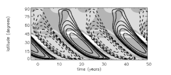
Figure 5: Time-latitude butterfly diagram for the model of Table 1 with a tachocline of constant width $d_{1}$$=$$0.05R_{\odot}$. The continuous (dashed) lines represent the positive (negative) strength of the toroidal field at the base of the solar convection zone (i.e. the top of the tachocline $r$$=$$R_{c}+d_{1}/2$). The lines are log spaced and cover the interval between $5\times 10^{4}$ $-$ $10^{5}$ G. The background gray scale represents the positive (clear) and negative (dark) radial field at the surface.

4.1 An ellipsoidal tachocline

As stressed in §1, so far, the exact location and width of the tachocline are still unknown. A good revision of the observational results and theoretical models of the tachocline can be found in Corbard et al. (2001). Some evidence for a prolate shape has been found by Antia et al. (1998) and Charbonneau et al. (1999), but this could be due to observational uncertainties or to a particular sensitivity to the inversion techniques employed to analyze these data (Corbard et al. 2001). Numerical simulations (Dikpati & Gilman 2001) have found that a strong magnetic stress ($B>10^{5}$ G) can pile the matter into the pole increasing the density and thus the width of the tachocline there. This could explain, in principle, the prolate shape, however, since a strong field is present only during the maximum of activity, this could suggest that the tachocline would have a varying shape through the cycle, becoming nearly prolate during the maximum activity.

In order to evaluate the effects of a potential prolate tachocline in a flux dominated dynamo model, we have introduced a latitudinal dependence on the width of the tachocline in equation (7), making it to vary from $d_{1}$(pole)$=$$0.07R_{\odot}$ to $d_{1}$(equator)$=$$0.02R_{\odot}$ (see left panel of Figure 6, top). This modification in the shape of the tachocline has the effect of decreasing the radial shear ${\partial\Omega/\partial r}$ at the high latitudes. If the appearance of strong toroidal fields at high latitudes were mainly sensitive to the radial shear, then one should expect that a reduction in ${\partial\Omega/\partial r}$ at those latitudes would reduce the amplification of the toroidal field. However the butterfly diagram depicted in Figure 6 (top), which was calculated for a prolate tachocline, shows no significant changes with respect to the diagram of Figure 5, for which a constant width tachocline was assumed. Besides, when an oblate configuration is considered instead (left panel of Figure 6, bottom), we find that the toroidal field is amplified to its maximum value only below the $60^{\circ}$ latitude (right panel of Figure 6, bottom). In other words, for an oblate tachocline, for which the radial shear is improved towards the higher latitudes, we find an inhibition in the generation of toroidal fields at those latitudes, contrary to what is commonly expected. Also, for both the oblate and the prolate tachoclines, the generation of toroidal fields at the low latitudes is practically the same, suggesting that ${\partial\Omega/\partial r}$ is not influencing the behavior of the toroidal field.

4.2 A thinner or a thicker tachocline?

Two interesting remarks can be pointed out from the results of Figure 6. On one hand, it does not seem to be posssible to reproduce the butterfly diagram with a prolate tachocline (i.e., with a thicker tachocline at higher latitudes), at least not for the assumed conditions. On the other hand, we find that the radial shear ${\partial\Omega/\partial r}$ does not seem to be contributing for the amplification of the toroidal magnetic field.

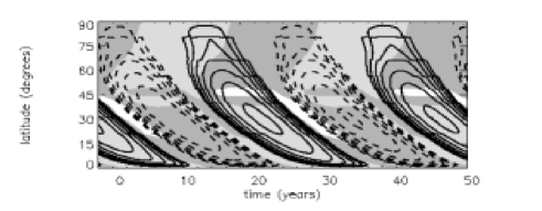
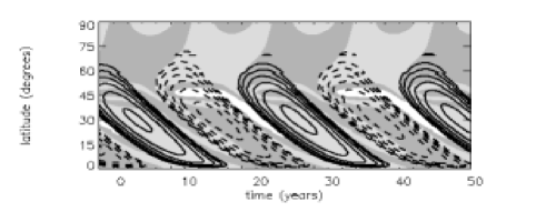
Figure 6: Angular velocity profiles and time-latitude butterfly diagrams for a prolate tachocline (top panel); and an oblate tachocline, (bottom panel). See the text for details. The contours specifications in the right panels are the same as in Figure 5. The tachocline in the left panels is represented by dashed lines.

In order to investigate the origin of this apparent paradox, we have considered again a spherical tachocline (with constant width), and then computed the components of the shear term on the RHS of equation (2). $({\bf B_{p}}\cdot\nabla)\Omega$$=$$B_{r}{\partial\Omega/\partial r}+B_{\theta}/r\,\partial\Omega/\partial\theta$, at a high latitude from the equator ($\theta$$=$$60^{\circ})$ , for $r$$=$$R_{c}$ (i.e., in the center of the tachocline where the radial shear is maximum) at a time when the radial magnetic field ($B_{r}$) inverts its polarity. At this time of the cycle, the action of the shear term upon the poloidal field generates new branches of toroidal field and establishes the morphology of this growing branch for the next phase of the cycle. We have also computed the toroidal magnetic field ($B$), at the same latitude when it reaches its maximum at the top of the tachocline. These quantities were computed as a function of the width of the tachocline ($d_{1}$) taken in the range of possible values that are inferred from the observations ($0.01R_{\odot}\leq d_{1}\leq 0.1R_{\odot}$; Corbard et al. (2001)), the results are depicted in Figure 7.

We note that the radial component, $B_{r}(\frac{\partial\Omega}{\partial r})$ (Figure 7$a$), actually tends to decrease with the increase of the width, as expected. But, more significant is the fact that its value is about two orders of magnitude smaller than that of the latitudinal component $\frac{B_{\theta}}{r}(\frac{\partial\Omega}{\partial\theta})$ (Figure 7$b$). Therefore, when a new toroidal field begins to be generated its growth is dominated by the latitudinal shear in eq. (2). Tests run for different latitudes revealed the same effect. This is confirmed by Figure 7$c$, which shows that the magnitude of the generated toroidal field at high latitudes varies with the width of the tachocline in a similar way to the latitudinal shear component (Figure 7$b$), attaining a maximum value at a width, $d_{1}$ that depends on the assumed magnetic diffusivity. This latter result will be explored in more detail in the next paragraphs.

The results above raise two new questions. Since the radial shear does not seem to be important for the amplification of the toroidal magnetic field, nor even at high latitudes, is the tachocline really participating in the dynamo process? And if yes, what is the real thickness of this layer? In the present model, the tachocline is not only the interface where the radial shear ${\partial\Omega/\partial r}$ is maximized, but also the place where the meridional flow penetrates and the magnetic flux tubes are stored and amplified before erupting by buoyancy effects to the upper layers, so that our answer to the first question is yes. In order to answer to the second question we can examine the amplitudes of the generated toroidal field at the latitude $60^{\circ}$, at the top of the tachocline in Figure 7$c$. It indicates that values of $d_{1}$$\lesssim$$0.02$$R_{\odot}$ and $d_{1}$$\gtrsim$$0.08R_{\odot}$ are appropriate to prevent the formation of strong toroidal fields at high latitudes, as required by the observations. But which value of $d_{1}$ is the best one? As we have mentioned above, the toroidal fields that develop at the high latitudes are also dependent of the adopted diffusivity profile. For a definitive answer, we have to wait for better helioseismic observations in the future, nonetheless, a more detailed scanning of the diffusivity parameters, as shown in the next section, can shed some light on this question.

4.3 Parameter dependence

Figure 7: Amplitude of the shear terms: a) $B_{r}\left(\frac{\partial\Omega}{\partial r}\right)$; b) $\frac{B_{\theta}}{r}\left(\frac{\partial\Omega}{\partial\theta}\right)$ at the time of inversion of the radial magnetic field, at a high latitude ($60^{\circ}$), at the center of the tachocline and c) the toroidal field $B$ at the time it reaches its maximum at the top of the tachocline as a function of the thickness of the tachocline. Dashed and continuous lines represent two different values of the turbulent diffusivity in the convection zone, $\eta_{c}$$=$$5\times 10^{9}$ cm² s^-1, and $2\times 10^{10}$ cm² s^-1 respectively (the continuous line corresponds to the value of Table 1).

The present model employed a large number of parameters and we have performed some tests in order to explore how sensitive the results above are to them. The meridional circulation term in equations (4)-(6) has two free parameters, the amplitude of the meridional flow at the surface, at middle latitudes, $U_{0}$, and the depth of the penetration of the meridional flow, $R_{p}$. While the first does not affect the strength of the generated magnetic fields (though it is very important to establish the period of the cycle), the second is able to change the latitude of formation of strong magnetic fields, as stressed by Nandy & Choudhuri (2002). We should note, however, that in this analysis we are assuming a weak penetration regime, and small variations around the value depicted in Table 1 do not change significantly the results above.

The $\alpha$ term, whose semi-empirical profile was chosen in order to better reproduce the observations (Figure 4), has only one free parameter, the amplitude, $\alpha_{0}$ (in equation 3.4). It determines the exact amount of poloidal field to be regenerated in order to support the cycle. We find that our model is generally very insensitive to variations to it.

For the diffusive terms of equation (7), it is possible to establish some constraints in the different regimes. For the most external layer, we have adopted a value for the diffusivity that has been obtained from the observations, so that it has been fixed in all the simulations. The value of the diffusivity at the radiative zone is not expected to affect the results either, but these can be sensitive to the assumed turbulent diffusivity at the convection zone ($\eta_{c}$), as indicated by Figure 7. We may choose an appropriate value for $\eta_{c}$ based on the period of the cycle and the magnitude of the generated fields. If the value of $\eta_{c}$ is too large, the system will enter in a diffusion dominated regime, thus reducing the period of the cycle in the butterfly diagrams. On the other hand, if $\eta_{c}$ is too small, it will lead to too large values of the radial field at the poles.

In Figure 8, we have plotted the maximum toroidal magnetic field at the top of the tachocline, at a latitude of $60^{\circ}$ (as in Figure 7$c$), as a function of the diffusivity $\eta_{c}$, taken in the range of values which are appropriate for the solar cycle. Different line styles correspond to different values of the tachocline width. The dotted line at $5\times 10^{4}$ G marks the limit between buoyant and no-buoyant magnetic flux tubes. If a curve is located above this limit, magnetic contours will appear above $60^{\circ}$ in the butterfly diagram, and this is not desired. The top and bottom panels of Figure 8 have been plotted for two different values of the parameter $r_{c}$ of the turbulent diffusivity profile of the convection zone (eq. 7). According to Figure 3, this is the transition radius between a weak and a strong turbulent regime. Though this value has been determined from helioseismic observations with high precision ($r_{c}$$=$$0.715R_{\odot}$), we have decided to vary it by $0.5$% in order to check the sensitivity of the results to it. In the top panel, $r_{c}$$=$$0.715R_{\odot}$ is the same value adopted in the previous Figures. In the bottom panel, we have displaced this value to $r_{c}$$=$$0.72R_{\odot}$ which means that a larger portion of the tachocline must lie in the less turbulent (sub-adiabatic) zone. Both, the top and the bottom panels indicate a similar behaviour for the different values of the tachocline width, but with a slight shift of the curves of the bottom panel towards larger diffusivity values, which are allowed only if the turbulent zone is smaller.

The top panel shows that a tachocline with a width of about $2$% of the solar radius or less will produce solar like butterfly diagrams for almost the entire diffusivity range. Intermediate widths, $d_{1}$$\simeq$$0.04R_{\odot}$$-$$0.06R_{\odot}$, are out of the allowed range of magnetic fields for any diffusivity, and larger widths between $\sim$$0.08R_{\odot}$ to $\sim$$0.1R_{\odot}$, will also produce butterfly diagrams which are in good agreement with the observations for $\eta_{c}$ from $2\times 10^{9}$ cm s^-2 to $1\times 10^{10}$ cm s^-2. The bottom panel also indicates that intermediate widths ($d_{1}$$\simeq$$0.04R_{\odot}$$-$$0.06R_{\odot}$) will produce inappropriate butterfly diagrams, while a thin enough tachocline ($d_{1}$$\lesssim$$0.02R_{\odot}$) will produce solar like butterfly diagrams for the entire range of appropriate diffusivities, and thicker tachoclines $d_{1}$$\simeq$$0.08R_{\odot}$$-$$0.1R_{\odot}$ will produce solar like results only for diffusivities in the $6\times 10^{9}$$-$$1.6\times 10^{10}$ cm² s^-1 interval. Computations made with $r_{c}$$=$$0.71R_{\odot}$ revealed a similar behaviour with a slight shift of the curves towards lower values of the diffusivity with respect to the $r_{c}$$=$$0.715$ panel (Figure 8, top).

Figure 8: Maximum of the toroidal magnetic field at the top of the tacholine as function of the diffusivity (in log-scale)at a latitude of $60^{\circ}$, The different line styles represent different widths of the tachocline $d_{1}$. The doted line represents the limit between buoyant and no-buoyant magnetic fields $5\times 10^{4}$ G, as explained in the text. Only the values below this line will appear in the desired latitudes. The top and bottom panels correspond to two different values of $r_{c}$ in the diffusivity profile, $r_{c}$$=$$0.715R_{\odot}$ (as in all previous Figures) and $r_{c}$$=$$0.72R_{\odot}$, respectively.

The butterfly diagrams plotted in Figure 9 for two spherical tachoclines, one with a thin width ($d_{1}$$=$$0.02R_{\odot}$, $\eta_{c}$$=$$5\times 10^{9}$ cm² s^-1, $r_{c}$$=$$0.72R_{\odot}$) and the other with a thick width ($d_{1}$$=$$0.08R_{\odot}$, $\eta_{c}$$=$$3\times 10^{9}$ cm² s^-1, $r_{c}$$=$$0.715R_{\odot}$) are the ones that better reproduce the observations.

We notice that the results above are also applicable to prolate and oblate tachoclines and naturally explain the results of Figure 6. In fact, since a prolate tachocline has a larger width at higher latitudes (top panel of Figure 6), then the toroidal field contours with strength between $5\times 10^{4}$ G and $1\times 10^{5}$ G develop over the entire hemisphere because the latitudinal shear (which dominates over the radial shear in all latitudes) increases towards the poles. On the other hand, in the oblate case (bottom panel of Figure 6) where the width is smaller at higher latitudes, the toroidal fields are suppressed there due to the smaller latitudinal shear, thus resulting in a more concentrated field distribution at the lower latitudes. However, the thickness of the tachocline at which the latitudinal shear has a maximum or minimum value depends on the assumed magnetic diffusivity profile. For the one assumed in Figure 6, a minimum value is obtained for a thinner tachocline (as in Figure 9, top) and therefore, the oblate configuration is the one that better reproduces the observations, but this scenario could change if a different diffusivity value had been adapted for the tachocline zone, than the one assumed in Figure 6. Note that the parameters used to built the butterfly diagram of the prolate configuration ($d_{1}$$=$$0.07R_{\odot}$ at the poles, $\eta_{c}$$=$$5\times 10^{9}$ cm² s^-1 ) lie in the forbidden zone of Figure 8. For example, according to the top panel of Figure 8, if we had taken $\eta_{c}$ between $2\times 10^{9}$ cm² s^-1 and $1\times 10^{10}$ cm² s^-1, then a prolate configuration with a tachocline width at the poles with $d_{1}$ between $(0.08-0.1)R_{\odot}$ would produce an appropriate butterfly diagram, because in this case even at the high latitudes, where the tachocline is thicker, the latitudinal shear would be small enough to suppress the toroidal fields there (like in Figure 9, bottom).

5 Conclusions

In this work we have explored the effects of variations in both the shape and the width of the solar tachocline in a flux-dominated kinematic solar dynamo model. First, employing an improved version of the numerical approach of Guerrero & Muñoz (2004) with a choice of more realistic diffusion and $\alpha-$effect profiles and assuming a tachocline with constant width $d_{1}$$=$$0.05R_{\odot}$, we were able to reproduce successfully some of the main features of the 11-year large scale solar magnetic cycle, like the phase lag between the toroidal and the poloidal fields, the correct period and magnetic field magnitudes (Figure 5). However remains of toroidal field component persisted at the high latitudes of the butterfly diagram for these initial conditions.

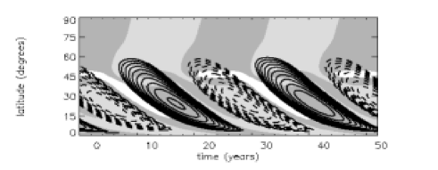
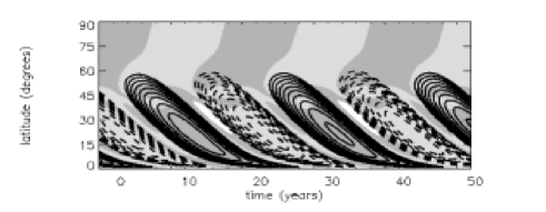
Figure 9: Angular velocity profiles and time-latitude butterfly diagrams for a thin ($d_{1}$$=$$0.02R_{\odot}$, $\eta_{c}$$=$$5\times 10^{9}$ cm² s^-1, $r_{c}$$=$$0.72R_{\odot}$) tachocline (top panel); and a thick ($d_{1}$$=$$0.08R_{\odot}$, $\eta_{c}$$=$$3\times 10^{9}$ cm² s^-1, $r_{c}$$=$$0.715R_{\odot}$) tachocline, (bottom panel). See the text for details. The contours specifications in the right panels are the same as in Figure 5. The tachocline in the left panels is represented by dashed lines.

Then, considering a prolate tachocline (Figure 6, top), with a larger width in the polar region, which implies a smaller radial shear ${\partial\Omega/\partial r}$ at these latitudes, we have obtained a butterfly diagram with similar distribution of the toroidal fields to that obtained with the constant width tachocline of Figure 5. On the other hand, when considering an oblate tachocline (Figure 6, bottom), we obtained a toroidal magnetic field with a latitudinal distribution that is in better agreement with the observations, with an absence of toroidal fields at latitudes higher than $60^{\circ}$.

In view of these surprising results, we computed the toroidal field and the radial and latitudinal components of the shear term (eq. 2) that is responsible for the amplification of the toroidal field, $({\bf B_{p}}\cdot\nabla)\Omega$$=$$B_{r}{\partial\Omega/\partial r}+B_{\theta}/r\,\partial\Omega/\partial\theta$ as a function of the width ($d_{1}$) of the tachocline at a high latitude, at a position where ${\partial\Omega/\partial r}$ should be maximum. The results suggest that the latitudinal component of the shear term dominates over the radial term for producing toroidal field amplification.

We have also found that these results are very sensitive to the adopted diffusivity profile, specially in the inner convection zone (which is characterized by the diffusivity $\eta_{c}$ and the radius $r_{c}$ of transition between a weak and a strong turbulent region). A diagram of the toroidal field at a latitude of $60^{\circ}$ versus the diffusivity at the convection layer for different values of the tachocline width has revealed that these fields are mainly eliminated for tachoclines with width $d_{1}$$\gtrsim$$0.08R_{\odot}$ and $\eta_{c}$$=$$2\times 10^{9}$$-$$1\times 10^{10}$ cm² s^-1, for $r_{c}$$=$$0.715R_{\odot}$; and $\eta_{c}$$=$$6\times 10^{9}$$-$$1.6\times 10^{10}$ cm² s^-1 for $r_{c}$$=$$0.72R_{\odot}$; or for $d_{1}$$\lesssim$$0.02R_{\odot}$ and practically any value of $\eta_{c}$ in the appropriate solar range. For intermediate values of $d_{1}$$\simeq$$0.04-0.06R_{\odot}$, strong toroidal fields should survive at high latitudes in the butterfly diagram and those values are therefore not suitable. The best fits to the observed butterfly diagram are shown in Figure 9 for a thin and a thick tachocline. We also conclude that a prolate tachocline can produce solar like results depending on the choice of the diffusivity profile and the adopted range of the tachocline width.

Finally, we should note that the poloidal magnetic field magnitudes are correctly reproduced except for a branch of strong radial fields migrating to the equator (see white features in the background grey scale of the butterfly diagrams of the figures). The formation of this branch is related to our non-local implementation of the $\alpha$-term. We will explore alternative forms for this term in future work.