DO QUASI-REGULAR STRUCTURES REALLY EXIST IN THE SOLAR PHOTOSPHERE?
I. Observational evidence

Abstract

Two series of solar-granulation images — the La Palma series of 5 June 1993 and the SOHO MDI series of 17–18 January 1997 — are analysed both qualitatively and quantitatively. New evidence is presented for the existence of long-lived, quasi-regular structures (first reported by Getling and Brandt (2002)), which no longer appear unusual in images averaged over 1–2-h time intervals. Such structures appear as families of light and dark concentric rings or families of light and dark parallel strips (“ridges” and “trenches” in the brightness distributions). In some cases, rings are combined with radial “spokes” and can thus form “web” patterns. The characteristic width of a ridge or trench is somewhat larger than the typical size of granules. Running-average movies constructed from the series of images are used to seek such structures. An algorithm is developed to obtain, for automatically selected centres, the radial distributions of the azimuthally averaged intensity, which highlight the concentric-ring patterns. We also present a time-averaged granulation image processed with a software package intended for the detection of geological structures in aerospace images. A technique of running-average-based correlations between the brightness variations at various points of the granular field is developed and indications are found for a dynamical link between the emergence and sinking of hot and cool parcels of the solar plasma. In particular, such a correlation analysis confirms our suggestion that granules — overheated blobs — may repeatedly emerge on the solar surface. Based on our study, the critical remarks by Rast [2002] on the original paper by Getling and Brandt (2002) can be dismissed.

1 Introduction

As reported previously by Getling & Brandt (2002; hereinafter, paper I), the procedure of time averaging applied to a 2-h interval of the 11-h La Palma series of granulation images (see below) reveals signs of long-lived, quasi-regular photospheric structures — “ridges” and “trenches” in the brightness distributions, which form systems of concentric rings or parallel strips. These systems resemble some roll patterns known from laboratory experiments on Rayleigh–Bénard convection and may be an imprint of the pattern of subphotospheric convection. It was also noted that averaging does not completely smear the image, which still comprises a multitude of granular-sized, light “blotches” against a darker background. In some cases, the time variations of intensity at the point corresponding to the averaged-intensity maximum in such a blotch and to a nearby minimum exhibit a tendency to anticorrelation. We interpreted all these findings as evidence for the presence of a previously unknown type of self-organization in the solar atmosphere.

After paper I appeared, Rast [2002] disputed our conjecture. He suggested that the features of granulation patterns reported by us are merely of statistical nature and do not reflect the structure of real flows. To substantiate this suggestion, he artificially constructed a series of random fields with some characteristic parameters typical of solar granulation. Rast claimed that the features of regularity described in paper I can be reproduced even if such artificial fields are used instead of real photospheric images. On this basis, he denied that our observations had any physical implications.

Here, a more extensive investigation of the quasi-regular structures is presented. In addition to the La Palma series, we consider a 45.5-h series of white-light images obtained with the SOHO MDI instrument. We analyse movies constructed by taking running averages on these two series of images, employ some techniques of algorithmic treatment of the images, and note remarkable features of spatio-temporal intensity correlation related to the structures.

Although some doubts about the reality of our elusive subject may still remain, the results that will be presented here and in a companion paper to be written in coauthorship with P. N. Brandt additionally testify to the actual existence of long-lived, quasi-regular structures. In particular, we can decline the critical remarks by Rast [2002].

2 Observations and Primary Data Reduction

The La Palma series of photospheric images was obtained by Brandt, Scharmer, and Simon (see Simon et al., 1994) on 5 June 1993 using the Swedish Vacuum Solar Telescope (La Palma, Canary Islands). It still remains unsurpassed in its duration (11 h), continuity (a constant, 21-s frame cadence), and quality (rms contrast varying between 6 and 10.6%).

The observations lasted from 08:07 to 19:07 UT on 5 June 1993. Images of a $118.7\times 87.9$ Mm² area of the solar photosphere, not far from the disk centre, were produced by the telescope in the 10-nm-wide spectral band centred at a wavelength of 468 nm. Frames were recorded every 21.03 s by a CCD camera with a pixel size of 0.125^′′, after selecting each of them as having the highest contrast among 55 images obtained during the first 15 s of the 21.03-s cycle. The resolution was typically no worse than about 0.5^′′.

The pre-processing of data included the following three principal steps. First, images were aligned by shifting the next image relative to any current one so as to maximize the correlation between them. Second, a destretching procedure based on the technique of local correlation tracking (November, 1986) was used to compensate for atmospheric distortions. Third, fast intensity variations were removed by subsonic Fourier filtering (Title et al., 1989) with a cutoff phase speed of 4 km s^-1. A Fourier transform technique was applied to interpolate the images to equal time cadence of 21.03 s. The entire series contains almost 1900 frames. For a more detailed description of the data-acquisition technique see Simon et al. (1994).

For our analyses, we use a subset of the series that covers an area of $43.5\times 43.5$ Mm² ($60^{\prime\prime}\times 60^{\prime\prime}$, or $480\times 480$ pixels) and an interval of length 8 h 45 min (1500 frames). The contrast of the printed images in this paper is artificially enhanced.

In addition to the La Palma series, we analysed the 45.5-h series obtained with the SOHO MDI instrument in 1997, from 17 January 00:01 UT to 18 January 21:30 UT (see Shine et al., 2000). This series contains white-light images with a resolution of about 1.2^′′ taken at a 1-min interval.

We mainly dealt with a subsonically filtered version of this series, which is free of five-minute oscillations and whose frames are fixed to a certain location on the solar surface. The filtered images are $304\times 480$ pixels in size, a pixel being about 0.6^′′ large. Accordingly, the area covered by an image measures $182^{\prime\prime}\times 288^{\prime\prime}$, or about $132\times 209$ Mm². Trenching patterns are especially pronounced in enlarged fragments of averaged images. For example, Figure 1 represents a cutout that contains $200\times 160$ pixels and measures about $87\times 70$ Mm².

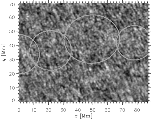
Figure 1: A sample of 2-h-averaged images of the SOHO MDI series with a pronounced trenching pattern. The light grey ellipse and circles mark concentric-ring structures. Multiple nearly-straight trenches and ridges form overall “hatching” diagonally downward to the right.

3 Movies

The very idea of implementing a study of well-correlated structures on the solar surface was suggested to us by a close examination of the movie representing the dynamics of granulation patterns that was obtained by Title et al. [1986] using the SOAP instrument of the Spacelab 2 optical laboratory on the Challenger space shuttle. If such a movie is viewed at a sufficiently low rate and especially in a back-and-forth playback mode over short intervals, signs of regularity become quite visible: the proper motions of granules appear to be organized in roll motions. While the roll widths are somewhat larger than the characteristic size of granules, the rolls are stretched over fairly long distances and, in some cases, form closed rings.

Generally, movies are very convenient for the visual identification of characteristic features of evolving patterns. Since time-averaged images that may visualize long-lived photospheric structures are a subject of our particular interest, we constructed movies of running-average sequences of images. In other words, each frame of such a movie is an image averaged over the same interval, while the central time of the averaging interval changes by a fixed increment between contiguous frames. If the averaging time is properly chosen, a careful inspection of running-average movies can enable us to detect features of interest and to follow their evolution. At the moment, we regard averaging times of about 1–2 h to be nearly optimal for the detection of quasi-regular structures. Mainly, we deal with 2-h running averages.

Our examination of running-average movies constructed from both the La Palma and SOHO MDI series has revealed numerous quasi-regular patterns, so that the presence of “trenching” patterns in the distributions of the time-averaged brightness no longer appears to be an unusual phenomenon. In particular, the distribution of light blotches and dark gaps between them is in many cases remarkably anisotropic. An example of a highly trenched pattern is given in Figure 1, where numerous ridges and trenches forming rightward downward “hatching” can be seen. In this case, the anisotropy in the distribution of linear chains of blotches is obvious (the averaging time is here 2 h). In addition, families of nearly concentric, not quite regular rings can be distinguished. They are marked with a light grey ellipse and light grey circles in the figure.

We emphasize that, in contrast to what Rast [2002] claims, his artificial random fields contain upon averaging only isolated linear features rather than families of such features and do not resemble averaged solar images.

Families of concentric rings are sometimes superposed with radial “spokes”, so that “web patterns” can be observed (see Figure 4). Ring and web patterns admit a hydrodynamic interpretation in terms of the development of certain instabilities of a larger-scale upwelling that can be associated with meso- or supergranules. We plan to consider this point elsewhere.

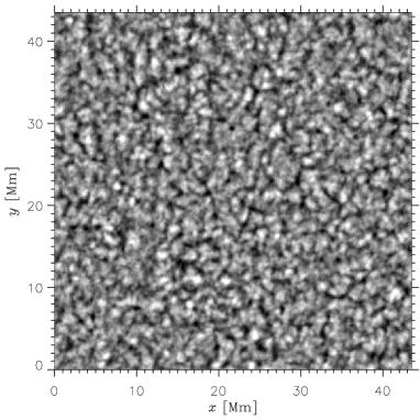
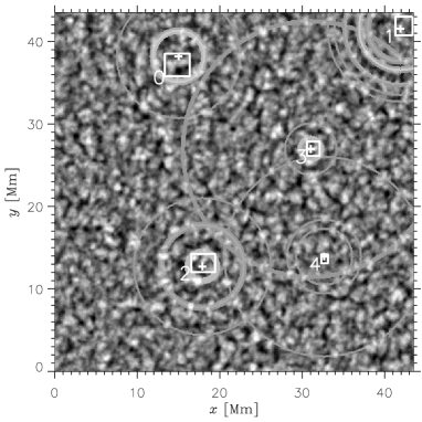
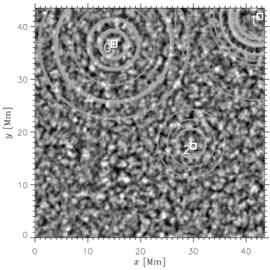
Figure 2: Top: A sample of 2-h-averaged images of the La Palma series. Middle and bottom: The same image superposed with patterns of azimuthally averaged intensity for the most likely positions of the centres of ring systems (crosses) detected by our algorithm. The scanned areas are marked with white rectangular frames and numbered. A common intensity scale is used for all centres in each panel.

Figure 3: Intensity as a function of the azimuthal angle $\phi$ at the radial distances where the azimuthally averaged intensity reaches its maximum (solid curve) and minimum (dashed curve), for three of the centres marked in Figure 2, middle. The area number and these radial distances (in pixels) are indicated at the upper edge of each panel. The horizontal lines correspond to the azimuthally averaged intensities (solid for the maximum and dashed for the minimum) and the vertical bars to the standard deviations.

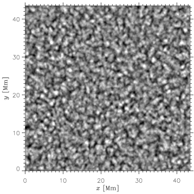
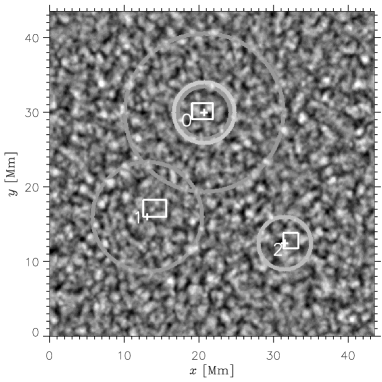
Figure 4: Top: A sample of 2-h-averaged images of the La Palma series. Bottom: The same image superposed with patterns of azimuthally averaged intensity for the most likely positions of the centres of ring systems (crosses) detected by our algorithm. The scanned areas are marked with white rectangular frames and numbered. A common intensity scale is used for all centres. A web pattern can be distinguished in the original image — its centre is located within the area labelled as 0 in the lower panel.

4 Algorithmic Treatment of Averaged Images

Our principal difficulty, which severely restricts possibilities of algorithmic detection of quasi-regular structures, stems from the very low signal-to-noise ratios. By the noise, we mean here the chaotic, blotchy background in which the quasi-regular patterns — the subject of our study — are “dissolved”. Up to now, none of the tested algorithms has been found to be universally capable of filtering out such a noise and detecting the ordered component of the averaged-intensity field. Nonetheless, some noteworthy features can be revealed using our algorithm described below. A possible alternative approach is based on using a software package intended for the detection of geological structures in aerospace images.

4.1 Analyses of azimuthally averaged brightness distributions

Our algorithm scans given rectangular areas in the image, uses each point as a trial centre, computes the radial distributions of the azimuthally averaged intensity, and plots rings at the local maxima of the averaged intensity.

Before constructing a time average, we normalize each individual image by setting the mean intensity to a certain level, universal to all images, and remove the residual large-scale intensity gradients. Within the averaged image, we delimit one or more rectangular areas in which the program will seek the most plausible position of the centre of a ring system. We also specify the maximum ring radius and the radial and azimuthal sizes of the bins that will be used to compute the brightness distribution.

Each area is scanned over two Cartesian coordinates, and each trial point (pixel) is regarded as the origin of an azimuthal coordinate system. The radial coordinate in this system is divided into small intervals — radial bins — and the intensity is averaged over each narrow annulus corresponding to a radial bin. This yields the radial distribution of the azimuthally averaged intensity referenced to the trial centre. If the centre lies in a light blotch, small-radius annuli may completely fall within this blotch, so that the averages over these annuli may be spuriously large. To avoid overestimating the role of the central pixels, the averaged intensities between the centre and the first local minimum next to the first local maximum are set equal to this local minimum. Among all radial distributions computed for the given area, the algorithm selects the one that exhibits the widest range of radial variation in the azimuthally averaged intensity. The corresponding trial centre is considered the best candidate for being the centre of some ring system.

If more than one area is selected in a given averaged image, the algorithm finds such a centre in each area and applies a common normalization to all radial distributions obtained for these centres. The ring pattern is visualized as follows. The absolute minimum of all distributions selected in the given image is subtracted from these distributions. In all of them, the radially averaged intensity is then set to zero wherever it does not exceed a chosen threshold value, and the resulting “apodized” distributions are additively superposed onto the original image. Except the two-dimensional maps of ring patterns thus obtained, two azimuthal distributions of the true (local) intensity are plotted for each centre; they correspond to the radial distances at which the azimuthally averaged intensities are maximum and minimum.

Figure 2 presents some results so obtained for one of the best available (in terms of the discernibility of structures) time-averaged images of the La Palma series. The image itself is shown in the upper panel. In two other panels, this image is superposed with the distributions of the azimuthally averaged intensity for some centres selected by the algorithm. The areas scanned by the algorithm are marked by white rectangles and numbered.

For some centres marked in the middle panel, Figure 3 shows the local intensity as a function of the azimuthal angle $\phi$, the azimuthally averaged intensity, and the standard deviations at the radii where the azimuthal averages are maximum and minimum. We see that the centres of clear-cut ring systems are characterized by especially large amplitudes of radial variations in the azimuthally averaged intensity. These are the centres marked in areas 0 and 1; the curves for area 2 in the middle panel and areas 0 and 1 in the bottom panel (not presented here) behave similarly. In contrast, the lowermost graph in Figure 3, shown for comparison, clearly illustrates the noisy character of the pattern around the centre found in area 4. This is consistent with the fact that no pronounced ring system has been detected for this area.

In both the middle and bottom panels of Figure 2, area 0 is associated with the same, most pronounced, ring system. The reasons for the dramatic difference in the corresponding radial distributions of the azimuthally averaged intensity are as follows. In the first case, the trial rectangular area was considerably larger, chosen in the hope that the formal criterion of maximum radial-variation range would be sufficient for the detection of a well-developed ring system. In the second case, the choice of the area was aimed at capturing the expected (“resonant”) centre of the visible ring system, while the centre selected in the first case fell outside this area; thus, the algorithm detected an intensity distribution outlining the visible ring pattern more clearly, although the range of radial variations in the azimuthally averaged intensity was somewhat smaller than in the first case. Obviously, the noise level is so high that it can accidentally yield a wider range for a centre other than the centre of the really present ring system. If, however, the algorithm, scanning the chosen area, passes through the resonant position of the trial centre, it detects the ring system quite successfully.

Likewise, area 1 is chosen in both cases so as to detect the pronounced ring system near the upper right corner of the considered region. In the bottom panel, area 1 is again smaller than in the middle panel and does not include the centre obtained using the larger area and marked in the middle panel. It is noteworthy, however, that the algorithm nevertheless detects the ring pattern that has nearly the same appearance whichever of these two trial areas is used. As can be seen from the graph for area 1 in Figure 3, a large difference between the maximum and minimum intensities is characteristic of this ring pattern; at the same time, the standard deviations are especially small, which is indicative of a relatively low noise level in this region.

Another example of applying our algorithm to time-averaged granulation images is given in Figure 4. Here, the centre detected in area 0 corresponds to a system that includes a pronounced ring about 8 Mm across, a much fainter ring (hardly discernible by eye) about 21 Mm across, and radial “spokes” within the smaller ring. On the contrary, the ring centred in area 1, which is very faint and isolated, simply represents the maximum of the radially averaged noise intensity and seems to have no physical meaning (such a maximum is necessarily plotted for any area provided the maximum intensity measured in units of the absolute maximum for all selected areas, exceeds some user-specified threshold). Apparently, this also applies to area 2, where the plotted ring is likewise isolated and faint.

Thus, although this algorithm is fairly sensitive to the level of noise in the analysed intensity field, not only may it be illustrative of qualitative differences between ring systems and purely chaotic patterns but it can also be used, with due care, to test hypotheses of the presence of faint ring systems. Further improvements of the identification criterion for ring patterns could enhance the potentialities of the algorithm.

A limitation of our algorithm lies in the fact that it assumes the structures to be strictly circular and cannot adapt itself to real, imperfect circles. To extend the scope for algorithmic treatment of structures in the solar granulation, attempts were made to apply a different approach.

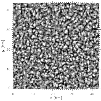
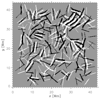
Figure 5: Processing of a sample of 1-h-averaged images of the La Palma series carried out by A.A. Buchnev using Salov’s algorithm. Left; original image: Right; detected light and dark linear structures on a grey background.

4.2 Application of an algorithm intended for aerospace-image processing

A few representative time-averaged images were tentatively analysed by A.A. Buchnev (Institute of Computational Mathematics and Mathematical Geophysics, Novosibirsk, Russia) using the software package developed at the same institute by Salov [1997] to detect linear and circular geological structures in aerospace images of the Earth’s surface (see also Buchnev et al., 1999). The algorithm that detects such structures uses a nonparametric statistical criterion, seeking lines in the image along which the intensity values are systematically higher or lower than the values at points located symmetrically on both sides of the line.

Figure 5 exemplifies the results of such a procedure. The program was run in the mode of seeking linear structures (lineaments). Curved features could generally be described as chains of lineaments of varying length. Both light and dark lineaments were detected, and their graphic representation is most descriptive if they are plotted on a grey background (Figure 5, right).

The most remarkable feature in this map of lineaments is a pronounced trenching pattern that includes families of parallel, alternating light and dark lineaments and chains of lineaments. If we ignore some purely disordered fragments of this pattern, we can note that, in some cases, lineaments forming different patches of this pattern can be connected by means of continuing them over the gaps between the patches, so that fairly extended families of lineaments can be detected. In particular, one of such families runs over the upper right quadrant of the frame, from the corner to the central region. It is to such objects that a physical meaning should be attributed in the first instance. Let us also note that most part of the lower left quadrant is encircled with a nearly elliptic contour intersected by a family of chains formed by parallel light and dark lineaments.

This example demonstrates that, although much care must be taken in using this image-processing procedure, the results obtained here show promise for the detection of hidden trenching patterns in time-averaged granulation images.

Figure 6: Pair of brightness-variation curves for the points of a local intensity maximum (solid curve) and a nearby minimum (dotted curve) chosen in a 2-h-averaged solar image.

5 Running-Average-Based Correlations

The strong brightness nonuniformity of the averaged granulation images (the presence of light and dark blotches) suggests that the probability of emergence of granules is likewise nonuniformly distributed over the solar surface, and granules “prefer” certain locations. From the standpoint of comprehending the physics of the phenomenon, it seems worthwhile to investigate the relationships between granule-emergence events at various points.

As thermal convection takes place in a horizontal fluid layer heated from below, the horizontal temperature distribution at a given height reproduces, to a first approximation, the horizontal distribution of the vertical velocity component at the same height. According to the viewpoint we hold (Getling, 2000), which agrees with some other analyses (Rieutord et al., 2001) and which will be further substantiated below, granules — blobs of overheated material — are relatively passive tracers of larger-scale convective motions, associated nevertheless with the small-scale “noise” in the velocity field. In this case, the distributions of temperature and vertical velocity over the photospheric surface on a mesogranular scale and up should be similar only when averaged over time. Likewise, we can expect the time-averaged field of the vertical velocity component to be mainly reflected by the time-averaged brightness field. Thus, steady convective upflows and downflows will appear light and dark in time-averaged images, respectively.

In paper I, we noted a remarkable property of the time variations of brightness at two points chosen in a 2-h-averaged granulation image (corresponding to nearly the same averaging interval as in the case of our Figure 2). One of these points corresponded to a local intensity maximum (which is in Figure 2 among the light blotches forming one of the light rings centred at point 0) and the other to a nearby minimum. The curves of brightness variation (not presented in paper I) are shown here in Figure 6. It can be seen that the intensity values at the two points exhibit apparent anticorrelation.

To check this immediate impression and in view of forming an idea of the dynamics of subphotospheric flows, it seems useful to calculate correlations between time variations of brightness at various points of the granular field. Assume that isolated hot blobs are present in the circulating material. Let the intensities at two points of the solar surface, presumably located at nearly the same streamline, be $I_{1}(t)$ and $I_{2}(t)$. Then some time scale $\tau$ of the order of the convective-circulation period should manifest itself in both these intensity variations. If there is no interference of other processes affecting the brightness at the considered location, $I_{1}(t)$ and $I_{2}(t)$ should correlate fairly well over a time interval $T$ corresponding to the lifetime of the local circulation system. If, however, such interference is present, the pattern of correlations may be substantially complicated and eventually smeared.

On the other hand, interference on a time scale $\mathcal{T}$ considerably longer than $\tau$, which would by itself produce an “interfering” correlation, can be eliminated as follows. Assume that, when computing the correlation, instead of the normal average values of $I_{1}(t)$ and $I_{2}(t)$ calculated over the whole time interval considered, we use their running averages obtained with a window wide enough to smooth out short-term variations on the time scale $\tau$ but narrow enough to retain the long-term variations on time scales comparable with $\mathcal{T}$. In this case, the fluctuations of $I_{1}(t)$ and $I_{2}(t)$ will be measured from the levels of the smoothed values, which experience the long-term variations, and these variations will not be taken into account in the resulting correlations. Thus, we shall obtain the correlation between the variations on the time scale $\tau$, while the effect of variations on the time scale $\mathcal{T}$ will be filtered out.

Let us consider the intensity variations at two points that are located not far apart and appear light and dark in the time-averaged image. Such points may prove to be the places of emergence and sinking of a hot blob. The lag between the brightness variations at the two points will correspond to the time taken by the blob to traverse the distance between these points. If the characteristic lifetime of the blob is larger than the circulation period, the correlation curve may exhibit additional correlation peaks separated from the main peak by this period (and, generally, its multiples). A moving temperature minimum at the same streamline, associated with cool material, will produce a negative extremum of the correlation function at a lag corresponding to the time interval between the passage of the hot blob through one point and the cool blob through the other.

To select correlations indicating that the two points may belong to a common circulation system, we compute running-average-based cross correlations between local intensity variations as follows. Let $x_{j}=(x_{0},...,x_{N-1})$ and $y_{j}=(y_{0},...,y_{N-1})$ be two data arrays with elements corresponding to $N$ instants of time $t_{j}=j\Delta t$, $j=0,...,N-1$. If we introduce a moving window of halfwidth $n\Delta t$, the running average of $x_{j}$ will be

$$\overline{x}_{i,n}=\left\{\begin{array}[]{lll}\frac{\textstyle{\sum\limits_{j=i-n}^{i+n}}x_{j}}{\textstyle\rule{0.0pt}{8.0pt}2n+1}&&\mbox{for}\ n\leqslant i\leqslant N\!-\!1\!-\!n,\\[10.0pt] \overline{x}_{n,n}&&\mbox{for}\ 0\leqslant i<n,\\[10.0pt] \overline{x}_{i,n}=\overline{x}_{N-1-n,n}&&\mbox{for}\ N\!-\!1\!-\!n<i\leqslant N\!-\!1\end{array}\right.$$

and similarly for $y_{j}$. We shall consider the running-average-based correlations between $x_{j}$ and $y_{j}$ defined as

$$P_{xy,n}(L)=\left\{\begin{array}[]{lll}\frac{\textstyle\sum\limits_{k=0}^{N-|L|-1}(x_{k+|L|}-\overline{x}_{k+|L|,n})(y_{k}-\overline{y}_{k,n})}{\textstyle\sqrt{\sum\limits_{k=0}^{N-1}(x_{k}-\overline{x}_{k,n})^{2}\sum\limits_{k=0}^{N-1}(y_{k}-\overline{y}_{k,n})^{2}}}&&\mbox{for}\ L<0,\\[35.0pt] \frac{\textstyle\sum\limits_{k=0}^{N-L-1}(x_{k}-\overline{x}_{k,n})(y_{k+L}-\overline{y}_{k+L,n})}{\textstyle\sqrt{\sum\limits_{k=0}^{N-1}(x_{k}-\overline{x}_{k,n})^{2}\sum\limits_{k=0}^{N-1}(y_{k}-\overline{y}_{k,n})^{2}}}&&\mbox{for}\ L\geqslant 0.\end{array}\right.$$

Obviously, for any $i$ and $n$, the substitution

$$\overline{x}_{i,n}\rightarrow\overline{x}\equiv\frac{\sum\limits_{j=0}^{N-1}x_{j}}{N},\quad\overline{y}_{i,n}\rightarrow\overline{y}\equiv\frac{\sum\limits_{j=0}^{N-1}y_{j}}{N}$$

(which sets the full width of the window equal to the length of the sample) reduces the running-average-based cross correlations to cross correlations defined in a standard way.

We present here three characteristic examples of correlations computed using the running-average technique. All of them refer to some “light”–“dark” pairs of points chosen in the concentric-ring system centred at point 0 in Figure 2. In each case, the light point corresponds to a local intensity maximum on a ridge in the 2-h-averaged image and the dark point is a nearby minimum in a trench next to the ridge. The correlation curves thus obtained admit a fairly definite physical interpretation. Figure 7 presents the results of employing the running-average technique with the window width varied. While the correlation curve obtained in a standard manner (top) does not contain any remarkable features and could be attributed to virtually independent brightness variations, the selection of short-term variations using windows as long as 39 min (bottom panel) reveals a strong anticorrelation between the light and the dark point with a nearly zero lag. Therefore, the brightening events at one point of the pair nearly coincide in time with darkening events at the other, while the sequence of events is far from periodic, and no appreciable correlation can be noted at lags other than zero. Thus, the updrafts of hot material seem to be physically related to downdrafts of cool material, although different couples of updraft and downdraft events appear uncorrelated with one another on the time scales considered. However, they are associated with the same region and should be controlled by the same local system of convective circulation. A correlation pattern of this type could arise if pairs of hot and cool blobs are located in opposite parts of a streamline.

Figure 7: Correlation curves obtained for a pair of points in the ring system centred at point 0 (Figure 2) using the standard technique (top) and running windows of various widths.

Figure 8: Correlation curves obtained for two other pairs of points in the ring system centred at point 0 (Figure 2) with a 39-min (top) and a 32-min (bottom) running window.

Even more interesting examples of correlation curves can be found in Figure 8. For both the top and bottom panels, the window widths (39 and 32 min, respectively) were chosen so as to obtain maximum absolute values of the correlation at its extrema. It can be seen that the two correlation functions are qualitatively similar, although they refer to two different pairs of points. The first one resembles a periodic function and exhibits fairly large extremum values of the correlation, while the second one is less regular. However, either has a negative extremum between lag values of $-24$ and $-23$ min and a positive one between $-8$ and $-7$ min. Moreover, the upper curve exhibits a series of sign-alternating extrema, which follow at an interval of 14–15 min. This pronounced tendency toward a periodic variation in the correlation coefficient, which is especially clear in the upper panel of Figure 8, can be regarded as evidence for a nearly periodic reoccurrence of light blobs (granules). If our interpretation is correct, we can use the first curve to estimate the circulation period, which proves to be 29–30 min. In the second case, such a determination is less certain, and the period may lie between 22 and 35 min.

Of course, the correlation curves are not always as regular as in the above examples. It should be kept in mind, however, that the choice of points was here almost arbitrary. In some cases, the points chosen to form a pair might really belong to different circulation systems (convection cells); in some others, they might lie at widely diverging streamlines although in the same system; finally, the circulation might locally be disturbed. However, the very existence of pairs that demonstrate such patterns of brightness correlation supports our suggestion that granules are hot blobs carried by convective circulation, which can even re-emerge on the photospheric surface.

6 Rast’s Comments on Paper I

As we already mentioned, Rast [2002] constructed a series of random fields similar to granulation patterns in some respects (mainly, in the mean values and standard deviations of certain random parameters). All of them were additive superpositions of $192^{2}$ randomly disposed two-dimensional Gaussians that randomly varied in amplitude and radius around given mean values. These values and the time scale of the evolution were chosen so as to mimic closely the corresponding parameters of the solar granulation. The sequence of such fields represented a continuous time evolution with persistent emergence of “new” Gaussian peaks and disappearance of “old” ones.

Averaging these fields over time revealed the following features. First, isolated rectilinear chains of light blotches of rectilinear dark lanes were discernible in some averages. Second, the “intensity”-variation curves for a local maximum and a nearby local minimum of the averaged “intensity” sometimes exhibited coincidence between a maximum of one curve and a minimum of the other. Third, the rms contrast of the averaged fields decreased with the averaging time in nearly the same manner as did the contrast of the averaged granulation images.

Based on these three properties of the artificial fields, Rast [2002] claimed that the emergence of the quasi-regular structures described in paper I and the apparent anticorrelation between the intensity variations at the “light” and “dark” points are purely statistical rather than physical effects. Let us discuss Rast’s reasoning in the context of our findings.

First of all, the isolated linear features observed in Rast’s averaged artificial fields have very little in common with the quasi-regular patterns revealed in the averaged images of the real solar granulation. The quasi-regular trenching patterns are formed by families of ridges and trenches in the brightness distributions — parallel strips, concentric rings, and, in some cases, radial “spokes”. Isolated linear features can also be found in the granulation images after time-averaging, but we make little account of those mainly because they may indeed be of statistical nature. In contrast, trenching patterns with signs of spatial periodicity (completely absent in the artificial fields) are of considerable interest from the standpoint of the hydrodynamics of subphotospheric layers.

Next, the correlations presented in Figures 7 and 8, unlike the visually compared brightness-variation curves, more definitely suggest that the convective circulation could be a common physical factor controlling the brightening events at one point and the darkening events at the other — in other words, the emergence of hot and cool blobs. Moreover, the correlations nearly periodic as a function of the time lag could naturally be attributed to the recurrent emergence of light blobs (granules) carried by the convective circulation. The characteristic circulation period of a blob estimated as the period of variation of the correlation coefficient is about two times as long as the characteristic lifetime of granules (10–15 min), and this fact indirectly supports our interpretation, according to which the granule should be visible as it traverses the upper half of its closed trajectory (streamline).

Finally, the important issue of the decrease in the rms contrast of averaged images with the averaging time could not be resolved based on the data presented in paper I. The spread in the original contrast values for individual granulation images is very wide, which makes it impossible to accurately compare the contrast-decrease laws for the real granulation and for the artificial random fields. As briefly noted by Brandt and Getling [2004] and will be shown more comprehensively in the forthcoming paper by Brandt and Getling, the accuracy of such comparisons can be substantially improved if the intensity of images is properly renormalized, so as to make the rms contrast and the mean intensity of each image equal to certain standard values. We apply this normalization procedure to the real granulation images of the La Palma series, to Rast’s artificial fields, and to two series of images obtained by numerically simulating the solar granulation. We see that, for the averaged granulation images, the curve of the contrast versus the averaging time is flatter than for the remaining three series. Moreover, the contrast of the averaged granulation images declines more slowly than according to the $t^{-1/2}$ law typical of the averages of random quantities ($t$ is the averaging time).

Thus, Rast’s arguments do not appear to apply to the real granulation patterns. Based on the above consideration, we can dismiss Rast’s criticism.

7 Discussion and Conclusion

We see that running-average movies constructed from both the La Palma and SOHO MDI series of granulation images are very useful in seeking long-lived, quasi-regular patterns. Families of straight or circular rings and also spoke and web patterns no longer appear to be unusual in time-averaged images of the solar granulation. They can be distinguished most clearly if the averaging time is about 1–2 h, so that their lifetimes are at least of this order of magnitude. Thermal convection of a Rayleigh–Bénard type is rich in a variety of flow patterns that it can form (see, e.g., Getling (1998) for a survey), and this physical mechanism could underlie the pattern-forming processes in the solar subphotospheric layers. It is worth remembering in this context that families of concentric rings distinguishable in some averaged photospheric images resemble the so-called target patterns observed in experiments on Rayleigh–Bénard thermal convection (see Assenheimer and Steinberg (1994) and a reproduction of their experimental photograph in paper I).

Applying our azimuthal-averaging algorithm to time-averaged images highlights, for some centres, systems of concentric annuli with substantially enhanced mean intensities. An algorithm of aerospace-image processing, tentatively employed to analyse time-averaged granulation images, can also be useful for the detection of trenching patterns in the brightness distributions.

Our analysis of correlations between brightness variations at the points corresponding to a local intensity maximum and a nearby intensity minimum in an averaged image suggests that blobs of hot material (which appear as granules) can repeatedly emerge on the photospheric surface, and their lifetime may be considerably longer than the lifetime of an individual observed granule. Another manifestation of this process could be the repeated expansion and fragmentation of granules associated with centres where the horizontal-velocity field has a strong positive divergence (Müller et al., 2001).

In view of the properties of granulation patterns described here and with due account for the contrast-variation laws reported by Brandt and Getling [2004] and planned to be analysed in more detail in the companion paper, we can dismiss the critical comments to paper I expressed by Rast [2002].

As we noted in paper I, signs of the prolonged persistence of granulation patterns were observed previously. Roudier et al. [1997] detected long-lived singularities (dark features — “intergranular holes”) in the network of supergranular lanes. They were continuously observed for more than 45 min, and their diameters varied from 0.24^′′ (180 km) to 0.45^′′ (330 km). Later, Hoekzema et al. [1998] and Hoekzema and Brandt [2000] also studied similar features, which were observable for 2.5 h in some cases.

An interesting parallel to our observation of concentric-ring patterns was reported by Berrilli et al. [2004], who analysed pair correlations in the supergranular and granular fields. They defined the pair-correlation function $g_{2}(r)$ so that the probability of finding a target supergranule or granule (identified by its barycentre) within an annulus of radius $r$ and width $\mathrm{d}r$ is $2\pi rg_{2}(r)\mathrm{d}r$, where $r$ is measured from the barycentre of a chosen reference supergranule or granule. Then the positions and heights of the peaks of such a function should reflect the topological order in the system. The computations of $g_{2}(r)$ based on observed supergranular and granular fields yielded qualitatively similar oscillating functions whose local amplitudes (measured from the mean $g_{2}(r)$ values) decrease with $r$ in each case from a maximum at some small $r$. This means that the patterns of supergranular and granular barycentres are most ordered at small $r$ and become less ordered at larger $r$. Such a behaviour of $g_{2}(r)$ could naturally be expected for supergranules, which form closely-packed patterns. In contrast, the presence of a similar (although not so perfect) order in the granulation field, especially pronounced in time-averaged granulation images, is much less trivial. (We note, however, that the authors themselves emphasize differences rather than similarities between the supergranular and granular fields in their topological orders.)

To all appearances, the interpretation of the quasi-regular patterns observed in the averaged granulation images should be based on analyses of the stability properties of cellular convection on meso- and supergranular scales. Variations in the local intensity of the convective circulation can affect the thermal structure of subphotospheric layers and, eventually, the fine structure of the velocity field in these layers. We plan to discuss these issues elsewhere.