Rounding up the wanderers: optimizing coronagraphic searches for extrasolar planets

Abstract

I derive analytic scalings for coronagraphic imaging searches for extrasolar planets. I compute the efficiency of detecting planets about any given star, and from this compute dimensionless distribution functions for the detected planets as a function of planet-star distance and distance to the host stars. I find the following for blind planet surveys: (1) the optimum wavelength is between 4000-5000 Å for Earth-like planets and 4200-5800 Å for Jovian planets; (2) between 21-32% of the number of planets per decade of radius can be detected with an optimized survey; (3) target stars should be ranked from greatest to least by their luminosity divided by distance to the sixth or eighth power, depending on the dominant source of noise for the survey; (4) surveys targeting all main sequence stars will detect $\sim$3 times as many planets as surveys only targeting G-type stars; and (5) stellar populations with different metallicities should have exposure times that vary with the cube of the metallicity. I apply these results to the current suite of proposed coronagraphic satellite telescopes, of which TPF-C is the most powerful, but a much smaller telescope, TOPS, may have a significant chance of detecting Earth-sized planets due to its small inner working angle and high throughput. The most significant uncertainty in these results is the noise contribution of Exo-zodiacal light. These results can be applied to designing coronagraphs, comparing proposed telescope designs, optimizing the observing strategies, determining the properties of detected planet populations, and selecting target stars.

1 Introduction

Now that extrasolar planets have been discovered with various indirect means (radial velocity, transits and microlensing, Mayor & Queloz, 1995; Konacki et al., 2003; Bond & et al., 2004), it is now a major goal of astronomy to directly detect extrasolar planets. Two means of imaging planets have been proposed: optical coronagraphy to capture light from the star scattered by the planet (Nisenson & Papaliolios, 2001; Kuchner & Traub, 2002; Kasdin et al., 2003; Brown et al., 2003; Stapelfeldt et al., 2005) and infrared interferometry to detect thermal emission from the planet (Leger et al., 1996; Fridlund, 2004; Kaltenegger & Fridlund, 2005). Here I carry out a detailed analytic analysis of the prospects for planet detection using optical coronagraphy with space-based telescopes.

A coronagraph enables planet detection by suppressing the light from the central star and suppressing the wings of the point spread function. The remaining stellar light is due to diffraction and scattering due to imperfections in the optics, which in some designs can be suppressed further by differencing images taken at different roll angles so that the speckles can be subtracted while the planet remains. Typical coronagraphic designs have an “inner working angle” within which the stellar PSF is too bright and the planet light is suppressed by the coronagraph. This sets the minimum angular scale at which planets can be detected relative to their host stars. Secondly, a coronagraph has a contrast between the wings of the PSF and the unobscured central brightness of the star, which, in addition to flux from local zodiacal light in our solar system and “exo-zodiacal” emission due to scattering by dust in the observed planetary system, sets the background at the position of the planet. These backgrounds set the maximum planet-star separation at which the planet can be detected as the planet flux decreases as the separation increases. Since the inner working angle is proportional to the wavelength of light, at shorter wavelengths planets can be detected closer to their host stars (where they are brighter) or around host stars at greater distances from Earth giving more stars that may be probed. However, the albedo and the stellar flux eventually decrease at short enough wavelengths, so at some point it does not pay to have higher angular resolution. The PSF contrast rises as the inverse of the square of the wavelength (due to the increase in phase error for shorter wavelengths, Angel & Woolf, 1998), which partly counteracts the benefits of short wavelengths if the wings of the PSF dominate the noise. If zodiacal or exo-zodiacal light dominate the noise, then shorter wavelengths means that the planet PSF will be more concentrated and thus less affected by the zodi/exo-zodi surface brightness. To compute the optimum wavelength of observation requires a knowledge of the sample stars, coronagraph properties, zodiacal and exo-zodicacal light, and survey parameters, as well as a model of the noise and coronagraph response. It is the goal of this paper to derive these quantities in as simple a manner as possible to elucidate the optimization of coronagraphic surveys for extrasolar planets.

As a measure of the success of a coronagraphic survey I use a straightforward metric: the total number of planets detected with specified properties. This allows a quantitative comparison of various telescope designs, survey strategies, observation wavelength, and choice of stellar targets. For the purposes of this study, I confine the analysis to blind, single-visit surveys, i.e. for which there are no known planets and each star is observed a single time.

Computations similar to those carried out here have been presented by Brown (2005), the primary difference being that Brown has focused on habitable terrestrial planets and his computations are numerical (using Monte Carlo realizations of simulated surveys) which require great computational expense to explore parameter space for different surveys. The formulae presented here target detection of planets at any separation from their host star and are analytic, allowing a rapid exploration of parameter space and faster optimization of surveys.

After introducing my assumptions about the planets (§3) and coronagraphs (§4), I compute the number of stars that can be surveyed (§6), the efficiency of detecting planets about a given star (§7), and the planet and star distance distributions (§7). I show how to choose the (dimensionless) survey volume (§8), how to rank target stars (§9), and how to optimize the wavelength of observation (§10). I use my results to compare various proposed coronagraphic imaging satellites (§11). I end with a discussion of how to weight observing time by metallicity (§12). In §13 I discuss the results and outline topics for further study. Two tables in the appendix summarize the notation used in the paper.

2 Planet detection requirements

To detect a planet with a coronagraphic telescope requires

• sufficient signal-to-noise, $S/N\geq(S/N)_{det}$. This should be chosen to be large enough that one is confident that a source is not due to a statistical fluctuation, so $(S/N)_{det}\sim 5-10$ should be sufficient given that tens to thousands of stars will be surveyed (although higher signal-to-noise may be required to provide convincing evidence of a planet, Gould et al., 2004).

• sufficient angular resolution, $\theta=r\sin{\alpha}/D\geq\theta_{IWA}$, where $D$ is the distance to the star, $\theta$ is the angular separation on the sky of the planet and star, $r$ is the planet-star separation, $0\leq\alpha\leq\pi$ is the phase angle of the planet ($\alpha=0$ at full phase), and $\theta_{IWA}$ is the inner-working-angle of the telescope within which a planet cannot be detected near the star.

These two conditions lead to the differential number of planets a survey can detect,

$${dN_{det}\over drdR_{p}d\alpha dMdXdD}={1\over 2}\sin{\alpha}\Omega_{s}D^{2}{dn\over dM}{dp\over dX}{df\over drdR_{p}}H(\theta-\theta_{IWA})H(S/N-S/N_{det}),$$ (1)

where $\Omega_{s}$ is the survey solid-angle, $D$ is the distance to surveyed stars ($\Omega_{s}D^{2}$ is the volume surveyed), $dn/dM$ is the stellar mass function (I assume in this paper that host stars are on the main-sequence), $dp/dX$ is the stellar metallicity probability distribution ($X$=[Fe/H]), $df/(drdR_{p})$ (defined below) is the frequency distribution of planets as a function of planet-star separation $r$ and planet radius $R_{p}$, and $H(x)$ is the Heaviside step function. I have assumed azimuthal symmetry for the detectability of planets around a given star, so the angular detection limit just depends on $2\pi r^{2}\sin{\alpha}/(4\pi r^{2})$. I have assumed that the stellar metallicity distribution is independent of stellar mass, hence the separate dependence on ${dn\over dM}$ and ${dp\over dX}$, and I have assumed that the planet size distribution is independent of stellar properties. The two step functions enforce $\theta>\theta_{IWA}$ and $S/N>S/N_{det}$. In the next section I specify my assumptions about the planet properties used in integrating this equation.

3 Planet parameter presumptions

In order to make a straightforward study of the dependence of coronagraphic searches on the properties of the coronagraph and telescope, I make some simple assumptions about the planet distribution and physical properties of the reflecting planets. I assume that the distribution of planets is independent of stellar spectral type, that the survey targets planets of a particular size $R_{p}$, and that the planet frequency is constant with the logarithm of radius,

$${df\over d\ln{r}dR_{p}^{\prime}}={f_{10}\over\ln{10}}\delta(R_{p}^{\prime}-R_{p}),$$ (2)

where $f_{10}$ is average number of planets per decade of radius and $\delta(x)$ is the Dirac delta function. Since I am assuming single-visit observations of each star, I can ignore the orbital parameters of each planet (such as eccentricity) and simply treat the density of planets near each star as a power law in radius once averaged over planet orbital elements. This implies a spatial density of $n(r)=f_{10}/(4\pi r^{3}\ln{10})$. Now, if the planets are distributed between an inner radius, $r_{in}$, and an outer radius, $r_{out}$, then the total fraction of stars with planets is $f_{p}=f_{10}[\ln(r_{out}/r_{in})/\ln(10)]$. I make this choice of planet distribution since the distribution of giant extrasolar planet periods is nearly proportional to $P^{-1}$ (Stepinski & Black, 2001; Tabachnik & Tremaine, 2002; Kuchner, 2004) which implies a constant number of planets per logarithmic radius interval, although one study suggests a shallower dependence (Lineweaver & Grether, 2003). We currently have no information on the distribution of terrestrial planets, but the constant $\ln{r}$ distribution seems to be a sensible choice as it is not biased towards detecting planets at either larger or smaller radius.

I compute the planet brightness with several assumptions. First, I assume that the brightness of the planet scales as the inverse square of its distance from the star. Second, I assume that the geometric albedo has a fixed spectral shape independent of planet-star separation. Third, I assume that the phase function is independent of planet-star separation and wavelength. I assume that all of these properties are independent of the planet mass, stellar spectral type, age and metallicity. Then, for a single exposure of a star with a planet, the number of photons detected from the planet is

$$Q_{p}\simeq Q_{*}p_{\lambda}\left({R_{p}\over r}\right)^{2}\Phi(\alpha),$$ (3)

where $p_{\lambda}$ is the geometric albedo (the fraction of the star’s flux reflected at full phase) of the planet at the observed wavelength $\lambda$ , $\Phi(\alpha)$ is the phase function (defined to be 1 at full phase when the star-planet-observer angle $\alpha=0$), and $Q_{*}$ is the number of photons from the star.

Planetary phase functions are fairly complex, but given the generality of this paper, I use the phase function $\Phi(\alpha)=\cos^{4}{(\alpha/2)}$. I refer to this as the “quasi-Lambert” phase function as it approximates the Lambert phase function, $\Phi(\alpha)=(\sin{\alpha}+(\pi-\alpha)\cos{\alpha})/\pi$, which is the phase function of diffuse scattering. The quasi-Lambert phase function has a mathematically convenient form that allows for analytic solution of the planet detection efficiency.

4 Coronagraph and survey assumptions

I assume that the coronagraphic search is carried out with direct imaging at a central wavelength $\lambda$ with a fractional band-pass $\Delta\ln{\lambda}<1$ with a mean throughput of $\epsilon(\lambda)$. The parameter $\epsilon$ includes all inefficiencies due to, e.g., partial obscuration of the mirror by the secondary, partial reflectance, partial coronagraphic obscuration, quantum inefficiency, observational overheads due to target acquisition and slewing, readout time, and multiple exposures for covering multiple angular regions for non-axisymmetric PSFs. I assume a circular telescope aperture of radius $R_{tel}$ with an inner working angle

$$\theta_{IWA}=\Theta_{IWA}\lambda/(2R_{tel}),$$ (4)

where $\Theta_{IWA}$ is a dimensionless number, typically 1.5-5, which relates the inner working angle and the ratio of the wavelength to the telescope diameter.

I assume that the telescope can achieve a contrast, $C(\lambda)$, which is constant in an annular region $\theta_{IWA}<\theta<\theta_{OWA}$, where $\theta_{OWA}\gg\theta_{IWA}$ is the outer working angle. The contrast is defined as the intensity ratio at a point in the PSF to the intensity of the centre of an unocculted stellar PSF (Kasdin et al., 2003). Since the phase errors scale as $\lambda^{-1}$, I assume that the contrast ratio scales as $C(\lambda)=C_{0}(\lambda_{0}/\lambda)^{2}$, where $\lambda_{0}$ is some reference wavelength (Malbet et al., 1995). This dependence results from gaussian errors in the phase (Angel & Woolf, 1998).

I assume that the telescope carries out a blind survey of nearby stars (i.e. not choosing stars that are known to have planets). I assume a constant exposure time of each star, $T_{exp}$ (if each planet is observed multiple times at different roll angles for speckle subtraction or covering the detection zone of the PSF, then $T_{exp}$ is the total time for exposures which include the planet). I assume that the survey has a fixed duration, $T_{s}$, which is typically of order several years, so that the total number of stars surveyed is

$$N_{s}=T_{s}/T_{exp}$$ (5)

(neglecting overheads, which are likely small due to long exposure times). Finally, I assume that each star is observed at one epoch so that the planet is at a fixed position. I relax the constant exposure time assumption later.

5 Signal-to-noise ratio

The total signal-to-noise for an observation scales as

$$S/N={Q_{p}\over\left(Q_{Z}+Q_{EZ}+Q_{PSF}+Q_{B}\right)^{1/2}},$$ (6)

where $Q_{p}$ is the total number of detected photons from the planet, $Q_{Z}$ is the noise contribution from zodiacal light, $Q_{EZ}$ is the noise contribution from exo-zodiacal light, $Q_{PSF}$ is the noise contribution from the wings of the stellar PSF, and $Q_{B}$ is the noise contribution from other sources (e.g. read-noise and dark current noise). This equation assumes the large-number photon limit applies, and since I am computing the number of planets that can be detected above a given signal-to-noise, I neglect the noise due to the planet (for planet characterization this should be included). For the remainder of this paper I will ignore $Q_{B}$ as I expect that detectors will be designed so that instrumental noise does not dominate.

The total number of photons detected from the unobscured star is

$$Q_{*}\simeq\pi R_{tel}^{2}\epsilon{L_{\nu}\over 4\pi D^{2}}\Delta\ln{\lambda}h^{-1}T_{exp}$$ (7)

where $L_{\nu}$ is the star’s specific luminosity (in erg s^-1 Hz^-1), $h$ is Planck’s constant and the other quantities are defined above. The noise due to zodiacal light is given by

$$Q_{Z}={\pi R_{tel}^{2}\epsilon L_{\odot,\nu}\Delta\ln{\lambda}h^{-1}T_{exp}\over 4\pi(1AU)^{2}}\tau_{Z}S_{fac}(\lambda/D_{tel})^{2},$$ (8)

where $\tau_{Z}$ (units of sr^-1) relates the solar flux to the zodiacal light surface brightness in the direction of ecliptic longitude and latitude $(\lambda_{ec},\beta_{ec})$ and $S_{fac}$ measures the PSF sharpness in units of $\lambda/D_{tel}$ (e.g. for optimal PSF fitting with an Airy disc point-spread-function, $S_{fac}=2.1$ ). The noise due to exo-zodiacal light is given by

$$Q_{EZ}={\pi R_{tel}^{2}\epsilon L_{\nu}\Delta\ln{\lambda}h^{-1}T_{exp}\over 4\pi(r\sin{\alpha})^{2}}\tau_{EZ}S_{fac}(\lambda/D_{tel})^{2},$$ (9)

where $\tau_{EZ}$ (units of sr^-1) relates the surface brightness of the exo-zodiacal light at the position of the planet to the flux of the star at the tangent point (integrated along the line of sight). Finally, the noise due to the wings of the PSF is given by

$$Q_{PSF}=Q_{*}C(\lambda)S_{fac}.$$ (10)

6 Simple survey scalings

Having outlined my various survey assumptions, I now derive some scaling parameters for coronagraphic surveys. I first assume that the noise is dominated either by $Q_{Z}$, $Q_{EZ}$, or $Q_{PSF}$; in §6.5 I will combine these to determine the scalings when all three sources of noise contribute.

There is a toroidal-shaped region surrounding the star within which the planet satisfies the signal-to-noise detection criterion (Figure 1). As the star becomes more distant the signal-to-noise for planets at separation $r$ decreases ($\propto D^{[-1,-2,-1/2]}$ in the [Zodi, Exo-zodi, PSF] limited cases), so the signal-to-noise detection region shrinks for a fixed exposure time. The angular resolution limit corresponds to a cylinder surrounding the star with the axis along the line of sight with a radius which grows as distance set by the inner working angle. Inside the torus and outside the cylinder is the planet detection zone. At some distance, $D_{max}(T_{exp})$ these two limits meet so that the torus is contained entirely within the cylinder - no planets can be detected for stars at $D>D_{max}(T_{exp})$ for a particular set of planet, stellar and telescope parameters. The distance $D_{max}$ sets the scale for the volume of stars that can be surveyed of a particular stellar type, so I next compute this for each of the three noise limits.

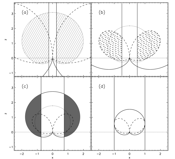
Figure 1: Cylindrical cross section of the region where planets can be detected for stars at a distance $D$ from the Sun for (a) $D=0.25D_{max}$; (b) $D=0.5D_{max}$; (b) $D=0.75D_{max}$; (d) $D=D_{max}$. Each panel is a 2-D cut through a 3-D region surrounding the star at the origin of each panel, where the units of the axes are $\theta_{IWA}D_{max}$. The observer is at $(x,z)=(0,-D\theta_{IWA}^{-1}D_{max}^{-1})$, and the inner working distance is indicated with vertical solid lines. The solid lines are for the Zodical dust noise limit, the dashed lines for the Exo-zodiacal noise limit, and the dotted lines for the PSF-limited noise limit. Note that for each noise limit, $D_{max}$ will be different, so each panel compares the three noise limits at different physical distances. The shaded regions are where a planet is detectable outside the inner working angle and inside the flux limit (I have only shaded one of the noise limits in each panel for clarity). Since panel (d) is at $D=D_{max}$, no planets can be detected.

6.1 Zodiacal dominated noise

When $Q_{Z}\gg Q_{EZ},Q_{PSF}$, to detect a planet requires $Q_{p}/Q_{Z}^{1/2}\geq(S/N)_{det}$. This implies

$$r\leq\left[{R_{p}^{4}p_{\lambda}^{2}\Phi(\alpha)^{2}Q_{*}{L_{\nu}\over L_{\odot,\nu}}\left({1AU\over D}\right)^{2}S_{fac}^{-1}\left({\lambda\over D_{tel}}\right)^{-2}\tau_{Z}^{-1}(S/N)_{det}^{-2}}\right]^{1/4}=r_{2,Z}.$$ (11)

The resolution limit requires

$$r\geq\Theta_{IWA}(\sin{\alpha})^{-1}\left({\lambda\over D_{tel}}\right)D=r_{1}.$$ (12)

Since detection requires $r_{1}\leq r\leq r_{2,Z}$, the limiting distance $D_{max}$ is set by $r_{1}=r_{2,Z}$ at $\alpha_{max}=60^{\circ}$ which is where the planet has the largest angular separation from the star (this is where the flux-limit and resolution limit meet in panel d of Figure 1). This gives

$$D_{max}=D_{Z}\equiv D_{tel}\left[{\cal G}{L_{\nu}^{2}T_{exp}(1AU)^{2}\over\lambda^{6}L_{\odot,\nu}\tau_{Z}\Theta_{IWA}^{4}}\right]^{\delta}.$$ (13)

where $\delta=1/8$ and

$${\cal G}={\textstyle\frac{1}{16}}R_{p}^{4}p_{\lambda}^{2}\Phi(\alpha_{max})^{2}\sin^{4}{\alpha_{max}}\epsilon\Delta\ln{\lambda}h^{-1}(S/N)_{det}^{-2}S_{fac}^{-1}.$$ (14)

6.2 Exo-zodiacal dominated noise

The noise due to exo-zodiacal light is difficult to estimate as the zodiacal dust content of other old stellar systems is unknown, except for a handful of infrared constraints with a sensitivity to dust $\sim$75 times as bright as our zodiacal dust cloud (Beichman et al., 2006). So, the largest uncertainty in planet detection efficiency is due to exo-zodiacal dust; until better constraints become available we will have to rely on educated guesses to estimate the contribution of this to planet detection noise.

For a planetary system with a dust cloud similar to that of the solar system, the surface brightness declines steeply with distance from the star, $\propto r^{-2.3}$, and varies significantly with the inclination angle and azimuth of the disk due to flatness of zodiacal dust cloud (Leinert et al., 1998). I will consider the case of largest noise: an edge-on disk. In this limit the equations simplify so that the exo-zodiacal surface brightness is just a function of the angular separation of the planet from the star. The detection limit for signal-to-noise, $Q_{p}/Q_{EZ}^{1/2}\geq(S/N)_{det}$, translates into a similar limit on radius which is

$$r\leq\left[{R_{p}^{4}p_{\lambda}^{2}\Phi(\alpha)^{2}Q_{*}D^{-2}\sin^{2}{\alpha}\ \tau_{EZ}^{-1}S_{fac}^{-1}D_{tel}^{2}\lambda^{-2}(S/N)_{det}^{-2}}\right]^{1/2}=r_{2,EZ}.$$ (15)

This equation applies when $\tau_{EZ}$ is independent of $r$ (which is nearly true for our zodiacal cloud). The resolution limit is the same, so setting $r_{1}=r_{2,EZ}$ at $\alpha_{max}$ (by coincidence, $\alpha_{max}=60^{\circ}$ in this case as well) gives the maximum distance

$$D_{max}=D_{EZ}\equiv D_{tel}\left[{\cal G}{L_{\nu}T_{exp}\over\lambda^{4}\tau_{EZ}\Theta_{IWA}^{2}}\right]^{\delta},$$ (16)

where $\delta=1/6$ here. For some stars with zodiacal dust that is more face-on, $D_{EZ}$ will be greater than this estimate. However, given the uncertainties in estimating $\tau_{EZ}$, a more complete calculation is unwarranted at this point.

6.3 PSF dominated noise

The signal-to-noise limit in the PSF noise dominated case, $Q_{p}/Q_{PSF}^{1/2}\geq(S/N)_{det}$, leads to the requirement that

$$r\leq\left[Q_{*}C^{-1}S_{fac}^{-1}p_{\lambda}^{2}R_{p}^{4}\Phi^{2}(\alpha)(S/N)_{det}^{-2}\right]^{1/4}=r_{2,PSF}$$ (17)

Setting $r_{1}=r_{2,PSF}$ at $\alpha_{max}$ allows us to solve for

$$D_{max}=D_{PSF}\equiv D_{tel}\left[{\cal G}{L_{\nu}T_{exp}\over\lambda^{2}C_{0}\lambda_{0}^{2}\Theta_{IWA}^{4}}\right]^{\delta},$$ (18)

where $\delta=1/6$ here. With these expressions for $D_{max}$ in three limits, I turn the planet detection expression into a dimensionless equation in §7.

6.4 Maximum number of stars

I now compute the the maximum number of stars that may be surveyed of a particular spectral type. If all stars surveyed are of a specific spectral type, i.e. $dn/dM^{\prime}=n_{*}\delta(M^{\prime}-M)$, then the total number of stars surveyed is $N_{s}=\Omega_{s}n_{*}D_{s}^{3}/3$, where $n_{*}$ is the number density of stars of the given spectral type, assumed to be constant, and $D_{s}<D_{max}$ is the limiting distance of surveyed stars. The total number of stars surveyed is also a function of the survey duration, $N_{s}=T_{s}/T_{exp}$.

The maximum number of stars that can be surveyed, $N_{max}$, can be found by equating these two expressions for $N_{s}$ and setting $D_{s}=D_{max}=D_{[Z,EZ,PSF]}$. I can solve for the maximum number of stars that can be surveyed in the three different noise limits

$$N_{max}=N_{[Z,EZ,PSF]}(T_{s})=\left[{\textstyle\frac{1}{3}}\Omega_{s}n_{*}D_{[Z,EZ,PSF]}(T_{s})^{3}\right]^{1\over 1+3\delta},$$ (19)

where $D_{[Z,EZ,PSF]}(T_{s})$ means that $T_{exp}$ is replaced by $T_{s}$ in equations (13), (16), or (18).

Since $N_{max}$ sets the characteristic scale for the number of stars to survey for a particular set of telescope, stellar, and planet parameters as well as total survey duration, it makes sense to scale the actual number of stars surveyed as

$${\cal N}=N_{s}/N_{max},$$ (20)

where ${\cal N}\la 1$. In §8 I determine the value of $\cal N$ which maximizes the number of detected planets and I estimate the total number of planets that can be detected, $N_{det}$, but it should be clear that $N_{det}$ scales with the maximum number of stars that can be surveyed, $N_{det}\propto N_{max}$, since the more stars that can be surveyed, the more planets can be detected. Although $N_{max}$ is defined only for a specific spectral type, in §9 I generalize to surveys of stars with multiple spectral types.

6.5 Summary

When all three sources of noise contribute, the general equation for $D_{max}(T_{exp})$ becomes:

$${D_{max}^{8}\over D_{Z}^{8}}+{D_{max}^{6}\over D_{EZ}^{6}}+{D_{max}^{6}\over D_{PSF}^{6}}=1,$$ (21)

which is a quartic equation in $D_{max}^{2}$ with solution

$$D_{max}(T_{exp}) = D_{Z}\left({G\over 2}-{V\over 4}+{1\over 2}\sqrt{{3V^{2}\over 4}-{V^{3}\over 4G}-G^{2}}\right)^{1/2}$$ (22)

$$G = \left({V^{2}\over 4}-{4\over S}+{S\over 3}\right)^{1/2}$$ (23)

$$S = {3\over 2^{1/3}}\left(\sqrt{V^{4}+256/27}-V^{2}\right)^{1/3}$$ (24)

$$V = {D_{Z}^{6}\left(D_{EZ}^{6}+D_{PSF}^{6}\right)\over D_{EZ}^{6}D_{PSF}^{6}}.$$ (25)

The ratio of the maximum distances in the three noise limits are

$${\cal D}_{1} = {D_{Z}\over D_{EZ}}=(1AU)^{1/4}\Theta_{IWA}^{-1/6}\lambda^{-1/12}\tau_{EZ}^{1/6}\tau_{Z}^{-1/8}L_{\nu}^{-1/24}{\cal G}^{-1/24}T_{exp}^{-1/24}L_{\nu,\odot}^{-1/8},$$ (26)

$${\cal D}_{2} = {D_{Z}\over D_{PSF}}=(1AU)^{1/4}\Theta_{IWA}^{1/6}\lambda^{-5/12}\tau_{Z}^{-1/8}L_{\nu}^{1/12}{\cal G}^{-1/24}T_{exp}^{-1/24}C_{0}^{1/6}\lambda_{0}^{1/3}L_{\nu,\odot}^{-1/8}.$$ (27)

The weak dependence on $L_{\nu}$ in these equations means that different spectral types will typically have similar noise properties.

Typically more than one source of noise dominates. However, the flux limits scale as $r_{2}\propto D^{[-1,-2,-1/2]}$ in the Zodi, Exo-Zodi, and PSF dominated cases, respectively, so if two noise limits are comparable near $D_{max}$, whichever grows fastest will dominate at smaller $D$.

When all three sources of noise contribute near $D_{max}$, the solution for $N_{max}$ is

$$\left({N_{max}\over N_{Z}}\right)^{11/3}+\left({N_{max}\over N_{EZ}}\right)^{3}+\left({N_{max}\over N_{PSF}}\right)^{3}=1.$$ (28)

This equation requires numerical solution of an eleventh order polynomial for $N_{max}^{1/3}$; however, to an excellent approximation,

$$N_{max}=\left(N_{Z}^{-10/3}+N_{EZ}^{-10/3}+N_{PSF}^{-10/3}\right)^{-3/10}.$$ (29)

7 Dimensionless distance distributions

The equations describing the detectable planets can be made dimensionless by scaling the star distance, $D$, as $\eta=D/D_{max}\left(T_{exp}\right)$ and the planet-star separation, $r$, as $\zeta=r/r_{max}$ where

$$r_{max}={\theta_{IWA}D_{max}\over\sin{\alpha_{max}}}.$$ (30)

Integrating the planet number density, $df/dr$ over the volume contained between the flux limits and inner working angle gives an expectation value for the number of planets detected about a star at a distance $\eta$ of

$${dN_{det}\over dMdXdD} = \Omega_{s}D^{2}{dn\over dM}{dp\over dX}2\pi\int_{0}^{\pi}\sin{\alpha}d\alpha\int_{0}^{\infty}dr{df\over dr}H(\theta-\theta_{IWA})H(S/N-(S/N)_{det})$$ (31)

$$= \Omega_{s}D^{2}{dn\over dM}{dp\over dX}E(\eta),$$ (32)

where $E(\eta)$ is the expectation value of the number of planets of radius $R_{p}$ detected for an observation of a single star with mass $M$, metallicity $X$, and distance $D=\eta D_{max}(T_{exp})$.

7.1 Expectation value as a function of distance

In the limit that one source of noise dominates at all distances, I can compute the integral of $E(\eta)$ over $\alpha$ and $r$, finding

$$E(\eta) = \phi f_{10}(\ln{10})^{-1}\left[3\ln{\left(x_{+}/x_{-}\right)}-(x_{+}-x_{-})\right],$$ (33)

$$x_{\pm} = (1+\Delta)\left[1\pm\left(2\Delta^{-1}-1\right)^{1/2}\right],$$ (34)

$$\Delta = \left(1+{3s\over 2\Gamma}+{3\Gamma\over 2}\right)^{1/2},$$ (35)

$$\Gamma = \left[s\left(1+\sqrt{1-s}\right)\right]^{1/3},$$ (36)

for $0\leq\eta\leq 1$, where $s=\eta^{1/(2\delta)}$ and $\phi=1/2$ applies in the PSF and zodi limits, while $\phi=1$ in the exo-zodi limit. This can be approximated accurately by $\tilde{E}(\eta)=\phi f_{10}{13\over 6\ln{10}}s^{-1/6}(1-s^{1/3})^{3/2}$. In carrying out this integral, I have neglected the cutoffs in the planet distribution at $r_{out}$ and $r_{in}$ which is appropriate if the peak of the detected planet distribution is well within these radii. If $df/d\ln{r}$ is a power law with radius rather than a constant, then $E(\eta)$ can be expressed in terms of Hypergeometric functions; however, for the reasons discussed above I stick to using a uniform $\ln{r}$ distribution. These three functions are plotted in Figure 2, which both show a rise at small $\eta$ as a larger volume is probed and fall at $\eta<1$ as the detection threshold is reached.

Figure 2: The expectation value for the number of planets detected as a function of distance for Zodi-limited (solid), Exo-zodi limited (dashed), and PSF-limited (dotted) surveys multiplied by the volume factor $4\pi\eta^{2}$ as a function of $\eta=D/D_{max}$.

In the limit ${\cal N}=1$, the total planet fraction can be computed analytically for the three noise limits. The fraction of surveyed stars with detected planets is

$${N_{det}\over N_{max}}=3\int_{0}^{1}\eta^{2}E(\eta)=f_{10}\begin{cases}5\pi 2^{-7/2}3^{-5/4}\left[\ln(10)\right]^{-1}\simeq 0.153&\text{Zodi-limit}\cr{64\over 135}\left[\ln(10)\right]^{-1}\simeq 0.206&\text{Exo-zodi limit}\cr{32\over 135}\left[\ln(10)\right]^{-1}\simeq 0.103&\text{PSF-limit}\end{cases}$$ (37)

So, depending on which noise-limit dominates 10-20% of planets per decade of radius will be detected around the stars that are surveyed. The detection inefficiency is due to both the spatial resolution limit and the flux limit which allow detection of planets within a limited range of radii, which I compute in the next section.

In the general case when all sources of noise contribute I have to integrate the dimensionless detection equations numerically. Defining

$$\eta_{Z} = {D_{max}\over D_{Z}},$$ (38)

$$\eta_{EZ} = {D_{max}\over D_{EZ}},$$ (39)

$$\eta_{PSF} = {D_{max}\over D_{PSF}},$$ (40)

where $0\leq\eta_{Z},\eta_{EZ},\eta_{PSF}\leq 1$ since $D_{max}\leq D_{Z},D_{EZ},D_{PSF}$, then,

$$\eta_{Z}^{8}+\eta_{EZ}^{6}+\eta_{PSF}^{6}=1,$$ (41)

which follows from equation (21). The equations for $r_{1}$ and $r_{2}$ become

$${r_{1}\over r_{max}} = \eta{\sin{\alpha_{max}}\over\sin{\alpha}},$$ (42)

$${r_{2}\over r_{max}} = \left[{\left(\eta_{EZ}^{12}+4\eta^{-4}(\eta_{Z}^{8}+\eta_{PSF}^{6}\eta^{-2})\left({\Phi^{2}\sin^{4}{\alpha}\over\Phi_{max}^{2}\sin^{4}{\alpha_{max}}}\right)\right)^{1/2}-\eta_{EZ}^{6}\over 2\left(\eta_{Z}^{8}+\eta^{-2}\eta_{PSF}^{6}\right){\sin^{2}{\alpha}\over\sin^{2}{\alpha_{max}}}}\right]^{1/2},$$ (43)

which is just a way of rewriting the resolution and signal-to-noise limits on radius. Using equation 41, I can eliminate $\eta_{Z}$ so that $r_{2}/r_{max}$ is just a function of $\eta$, $\eta_{EZ}$, $\eta_{PSF}$ and $\alpha$. With these definitions, the planet expectation value for a star at distance $\eta$ is given by

$$E(\eta,\eta_{EZ},\eta_{PSF})={f_{10}\over 2\ln{10}}\int_{x_{-}/2-1}^{x_{+}/2-1}d(\cos{\alpha})\ln{\left({r_{2}\over r_{1}}\right)},$$ (44)

where $x_{\pm}=4\cos^{2}{\alpha_{\pm}\over 2}$ are given by equation (33), but with $s=\eta^{3}\left[1-\eta_{Z}^{8}(1-\eta^{2})\right]^{1/2}$ ($\alpha_{\pm}$ are the angles where the resolution limit crosses the flux limit). I have not found an analytic solution to this integral, so I integrate it numerically below. The shape is qualitatively the same as in the three noise limits since all three have very similar shapes.

7.2 Radius distribution of planets

In the limit ${\cal N}=1$, the radial distribution of detected planets can be computed analytically in the Zodi and PSF noise limited cases, assuming that all stars observed are of a particular spectral type (e.g. G stars). For the Zodi limit,

$${dN_{det}\over d\zeta}={\Omega_{s}n_{*}D_{max}^{3}f_{10}\over 3\ln{10}}\left[{\zeta^{4}(1-\zeta^{4})(1+9\zeta^{4})\over(1+3\zeta^{4})^{3}}+{\zeta^{2}\over 2\sqrt{3}}\cos^{-1}\left({3\zeta^{4}-1\over 3\zeta^{4}+1}\right)\right].$$ (45)

The Exo-zodi case can be computed analytically in terms of Hypergeometric functions, but an excellent analytic approximation is

$${dN_{det}\over d\zeta}={\pi^{2}\Omega_{s}n_{*}D_{max}^{3}f_{10}\over 4\ln{10}}\left({1\over\zeta^{-2/g}+\zeta^{7/g}}\right)^{g},$$ (46)

where $g=1.9$ provides a good fit to the numerical curve. For the PSF limit,

$${dN_{det}\over d\zeta} = {\Omega_{s}n_{*}D_{max}^{3}f_{10}\over 2\zeta\ln{10}}\left[\frac{w^{6}}{\zeta^{6}}\left(\frac{1}{3}-\frac{3w}{7}\right)+{w^{2}\over 6}\left(1-{3w\over 2}\right)\left(1-6w+{9w^{2}\over 2}\right)+{\zeta^{3}\over\sqrt{27}}\cos^{-1}\left({3w\over 2}-1\right)\right],$$ (47)

$$w = \zeta^{3}\left[\Sigma-\Sigma^{-1}\right],$$ (48)

$$\Sigma = \zeta^{-1}\left(2+\sqrt{\zeta^{6}+4}\right)^{1/3}.$$ (49)

These distributions are plotted in Figure 3. All three distributions peak near $\zeta=1$ since the largest number of stars surveyed are near $D_{max}$ where the sensitivity is concentrated near $\zeta=1$ since this is near where the resolution and flux limits meet. Each of these curves approaches the same value at small $\zeta$ since the planets closest to the star are limited by resolution, which is independent of the phase function, scaling as $\propto\zeta^{2}$. At large $\zeta$, planet detection is flux-limited which scales as $r_{2}\propto D^{-b}$ where $b=[1,2,1/2]$ in the Zodi, Exo-zodi, and PSF noise limits. The planets at largest separation are detected for the closest stars, so it is straightforward to show that $dN_{det}/d\zeta\propto\zeta^{-(3/b+1)}=\zeta^{[-4,-5/2,-7]}$ in the Zodi, PSF and EZ limits, which is indeed the slope of the lines at large $\zeta$. Since the EZ flux limit grows most slowly with radius, the observed slope will generally be $\propto\zeta^{-7}$.

Figure 3: The expected distribution of the detected planet-star separations $\zeta=r\sin{\alpha_{max}}/[\theta_{IWA}D_{\max}]$ for the Zodi-limit (solid line), Exo-zodi limit (dashed line), and PSF-limit (dotted line) for surveys of a single stellar type, constant exposure time per star, and ${\cal N}=1$.

8 Maximizing over exposure time and survey volume

I assume for the time being that the telescope observes a single type of star at a single wavelength. Then, if fewer stars are observed out to a distance $D_{s}<D_{max}$ (i.e. ${\cal N}<1$), more time can be spent on each star making it possible to detect more planets since these stars are closer. Furthermore, it may pay to vary the exposure time with the distance to the star, say $T_{exp}\propto D^{-\kappa}$. Well, it turns out that choosing $\kappa=0$ and ${\cal N}=1$ is close to optimal. By increasing $\kappa$ to $\sim$0.5 (i.e. spending more time on closer stars) the total number of planets found can be increased by only $\sim$0.5% compared to the $\kappa=0$ case (for either $\delta=1/6$ or $1/8$). The reason is that the most planets are detected near $D_{s}$ due to the larger volume at larger distance, but because these stars are more numerous, they also primarily determine what the exposure time should be, so the total planet sensitivity at that distance is roughly constant. By making $\kappa$ slightly negative, then you can detect slightly more planets around closer stars, but this is counterbalanced by the fewer planets detected around more distant stars, and thus the total number of planets detected remains nearly constant. One advantage of spending more time on closer stars is that there will be more detections at higher signal-to-noise. Specifically, the number of stars with $S/N$ above $(S/N)_{det}$ scales as $(S/N)_{det}^{-1/(1+\delta\kappa)}$. Since this has a weak dependence on $\kappa$, the gain is not significant, so for the rest of the paper I assume a uniform exposure time with distance, i.e. $\kappa=0$.

A reduction in the number of stars can lead to an improvement in the number of planets detected as more time is spent observing closer stars. Figure 4 shows the dependence of $N_{det}$ on ${\cal N}$ computed from

$${N_{det}\over N_{max}}=3{\cal N}^{-3\delta}\int_{0}^{{\cal N}^{1/3+\delta}}d\eta\eta^{2}E(\eta)$$ (50)

for each of the three noise limits. For the zodi-limited case, I find ${\cal N}=0.59$ optimizes the total number of planets detected with an increase in the number of planets by $\sim$11% over the value at ${\cal N}=1$, while in the Exo-zodi and PSF limited cases, ${\cal N}=0.54$ is optimum with an increase in the number of detected planets by $\sim$16% over the value at ${\cal N}=1$. Even though only about half the number of stars are surveyed, the planet detection fraction roughly doubles causing a larger number of planets detected. In terms of distance, this corresponds to observing stars out to $D_{s}\sim 0.75D_{max}$ rather than out to $D_{max}$.

For the general case where all three sources of noise contribute, one must optimize

$$N_{det}({\cal N},{\cal D}_{1},{\cal D}_{2})=\left(\Omega_{s}n_{*}D_{max}^{3}(1)\right){D_{max}^{3}({\cal N})\over D_{max}^{3}(1)}\int_{0}^{{\cal N}^{1/3}D_{max}(1)/D_{max}({\cal N})}d\eta\eta^{2}E(\eta,\eta_{EZ},\eta_{PSF}),$$ (51)

where I have evaluated ${\cal D}_{1},{\cal D}_{2}$ at ${\cal N}=1$, i.e., at $T_{exp}=T_{s}/N_{max}$. The first term in parentheses is equal to $3N_{max}$. The Zodi-noise dominated case is for ${\cal D}_{1}={\cal D}_{2}=0$ or $\eta_{Z}=1,\eta_{EZ}=0,\eta_{PSF}=0$, while the Exo-zodi noise dominated case is for ${\cal D}_{1}=\infty$, ${\cal D}_{2}=0$ or $\eta_{Z}=0,\eta_{EZ}=1,\eta_{PSF}=0$, and the PSF-noise dominated case is for ${\cal D}_{1}=0$ and ${\cal D}_{2}=\infty$ or $\eta_{Z}=0,\eta_{EZ}=0,\eta_{PSF}=1$. The quantities $(\eta_{EZ},\eta_{PSF})$ can be expressed as a function of $[{\cal N},{\cal D}_{1},{\cal D}_{2}]$ with the relations

$$\eta_{EZ}^{6} = y^{3}{\cal D}_{1}^{6},$$ (52)

$$\eta_{PSF}^{6} = y^{3}{\cal D}_{2}^{6},$$ (53)

$$y = (1-\eta_{EZ}^{6}-\eta_{PSF}^{6})^{1/4}$$ (54)

$$y^{4}+{\cal R}y^{3}-{\cal N}^{-1} = 0,$$ (55)

$${\cal R} = {\cal D}_{1}^{6}+{\cal D}_{2}^{6}.$$ (56)

Coincidentally, the equation for $y$ is same as the equation for $(D_{max}/D_{Z})^{2}$ (equation 21). For a grid of values of $[{\cal D}_{1},{\cal D}_{2}]$ I solve these equations for $\eta_{EZ},\eta_{PSF}$ as a function of ${\cal N}$ and then numerically compute $E(\eta,\eta_{EZ},\eta_{PSF})$ and $N_{det}[{\cal N},{\cal D}_{1},{\cal D}_{2}]$.

I have carried out this numeric integration and then maximized $N_{det}$ with respect to ${\cal N}$. I find that the optimum values of ${\cal N}$ vary from 0.54-0.60 for the entire range of ${\cal D}_{1,2}$, with a mean of 0.57 and standard deviation of 0.02. So, in optimizing surveys I will just use the mean value of ${\cal N}=0.57$ since this only leads to a small error of at most 5%. The optimum value of $N_{det}$ varies by a factor of 2 (between the PSF and Exo-zodi limits, equation 37), so I have fit an equation to the numerical results:

$${N_{det}\over N_{max}}\approx f_{10}a_{1}\left[\ln{\left(\eta_{EZ}^{12}+4a_{0}^{-4}(1-\eta_{EZ}^{6}+\eta_{PSF}^{6}(a_{0}^{-2}-1)\right)^{1/2}-\eta_{EZ}^{6}\over 2(1-\eta_{EZ}^{6}+\eta_{PSF}^{6}(a_{0}^{-2}-1))}\right]^{1/2},$$ (58)

where $a_{0}=0.4249$ and $a_{1}=0.1287$. This equation ranges from 12%$f_{10}$ (for PSF-dominated noise with $\eta_{PSF}=1$) to 24%$f_{10}$ (for Exo-zodi dominated noise with $\eta_{EZ}=0$) and it agrees with the numerically computed values of $N_{det}$ within $<1$% fractional error! The number of stars being surveyed is $N_{s}={\cal N}N_{max}$, so the planet detection fraction of stars surveyed is actually [29%,44%,21%]$f_{10}$ in the [Zodi,Exo-zodi,PSF] cases; in practice the detection fraction will range between these values.

Figure 4: The dependence of the number of detected planets, $N_{det}$ on the number of stars surveyed, ${\cal N}$, both in terms of $N_{max}$. Solid line is for the Zodi limit, dashed line is for the Exo-zodi limit, and dotted line is the PSF limit.

9 Optimizing the choice of stars

Up until now, I have assumed that all stars are identical: same radius, same spectral shape, same luminosity, same planet frequency. However, surveys will be carried out for stars with a wide range of properties, so the question is: which are the best to observe?

The answer to this should be obvious: prioritize the stars which have the highest probability for detection of planets. For a particular survey telescope, planet type, and exposure time, $E(\eta,{\cal D}_{1},{\cal D}_{2})$ should be computed for each star and then stars can be ranked in decreasing order of $E$. If one particular source of noise is expected to dominate for all stars, then computation of $E$ can be sidestepped and stars can be ranked just based on the survey properties.

To do this, I define a new parameter

$$\beta\propto\eta^{-1/\delta},$$ (59)

that depends solely on the properties of the stars at the observational wavelength used in computing $\eta$,

$$\beta\equiv\begin{cases}L_{\nu}^{2}L_{\odot,\nu}^{-1}D^{-8}\tau_{Z}^{-1}&\text{Zodi-limit}\cr L_{\nu}D^{-6}\tau_{EZ}^{-1}&\text{Exo-zodi limit}\cr L_{\nu}D^{-6}&\text{PSF-limit}\end{cases}$$ (60)

Then, to choose stars I can simply rank stars from largest $\beta$ to smallest $\beta$ and observe in this order to maximize the number of detected planets. The parameter $\beta$ has the advantage that it can be defined independent of the parameters of any particular survey so that the ranked list of stars simply depends on the wavelength of observation and dominant noise.

For now, I will assume that the planet frequency is independent of stellar type and that stars are chosen of the same metallicity. For a given stellar type of uniform density one can show that $N(>\beta)=N_{\beta}\beta^{-3\delta}$. The normalization, $N_{\beta}$, is computed from

$$N_{\beta}\equiv{\Omega_{s}\over 3}\int dM{dn\over dM}\begin{cases}L_{\nu}^{3/4}L_{\odot,\nu}^{-3/8}\int d\tau_{Z}p(\tau_{Z})\tau_{Z}^{-3/8}&\text{Zodi-limit}\cr L_{\nu}^{1/2}\int d\tau_{EZ}p(\tau_{EZ})\tau_{EZ}^{-1/2}&\text{Exo-zodi limit}\cr L_{\nu}^{1/2}&\text{PSF-limit},\end{cases}$$ (61)

where $p(\tau_{Z})d\tau_{Z}$ is the probability distributions of $\tau_{Z}$ for the local zodiacal light; similarly, $p(\tau_{EZ})d\tau_{EZ}$ is the probability distribution for exo-zodiacal light (both assumed to be independent of stellar spectral type). I measure $L_{\nu}$ in units of $4\pi$ Jy pc² and $D$ in units of pc.

For computing $N_{\beta}$ I use the present-day disc mass function of main sequence stars given by Reid & Hawley (2005), the mass-temperature and radius-temperature relations given by Harmanec (1988), and stellar atmosphere models given by Hauschildt et al. (1999). My computed $N_{\beta}(\lambda)$ is shown in Figure 5 where it is compared with a model of the disc luminosity function of dwarf stars in $B,V,R,I$ and $K$ (Jarrett et al., 1994). I have checked that this result agrees with the sample of stars from Allende Prieto & Lambert (1999) (which is only complete for $T_{eff}>6000$ K, so I have only compared in this range of temperatures). About half of $N_{\beta}$ is due to low temperature stars ($T_{eff}<5000K$) in the $I$-band, while more than one third is due to these stars in $B$ and $V$. This indicates that late-type stars should be included in coronagraphic planet searches due to their greater number and thus greater proximity. This function can be used to compute the optimum wavelength of observation as shown below.

With $N_{\beta}$ in hand, the maximum number of stars to survey is

$$N_{max}=\begin{cases}N_{Z}=\left(N_{\beta}^{8/3}{\cal G}D_{tel}^{8}T_{s}[1AU]^{2}\lambda^{-6}\Theta_{IWA}^{-4}\right)^{3/11}&\text{Zodi-limit}\cr N_{EZ}=\left(N_{\beta}^{2}{\cal G}D_{tel}^{6}T_{s}\lambda^{-4}\Theta_{IWA}^{-2}\right)^{1/3}&\text{Exo-zodi limit}\cr N_{PSF}=\left(N_{\beta}^{2}{\cal G}D_{tel}^{6}T_{s}\lambda^{-2}C_{0}^{-1}\lambda_{0}^{-2}\Theta_{IWA}^{-4}\right)^{1/3}&\text{PSF limit},\end{cases}$$ (62)

where ${\cal G}$ is defined in equation 14. As before, if all three noise sources contribute then $N_{max}$ can be computed from equation 28 since ${\cal D}_{1},{\cal D}_{2}$ are weakly dependent on spectral type. Now, as in the case of a survey of stars uniform stellar type, the number of detected planets can be increased slightly if the number of stars surveyed is ${\cal N}=N_{s}/N_{max}=$54-59%. So, the cutoff is determined by

$$\beta_{s}=\left[{N_{\beta}\over{\cal N}N_{max}}\right]^{1/(3\delta)}.$$ (63)

So, all stars with $\beta>\beta_{s}$ can be chosen to optimize the survey. This guarantees that all stellar types will have a cutoff in distance at the same fraction of $D_{max}$. Since I am assuming a constant exposure time per star, then the time will be divided up between various spectral types according to the integrand in equation 61. For example, in the PSF-limited case, stars of luminosity $L_{\nu}$ will have time spent $dT_{s}\propto(dn/dM)L_{\nu}^{1/2}dM$.

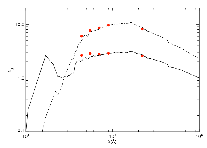
Figure 5: Normalization of $\beta$ distribution as a function of wavelength for main sequence stars with $\Omega_{s}=4\pi$, solid line is Zodi-limit while dashed-dot is Exo-zodi and PSF limits. The large dots are computed using the $B,V,R,I$ and $K$ band luminosity functions of nearby main sequence stars. For the Zodi and Exo-zodi limits, $\tau_{Z,EZ}$ has been set to one. The units of $N_{\beta}$ are chosen so that the specific luminosity has units of $4\pi$ Jy pc² and distance has units of pc.

10 Optimizing the wavelength of observation

Since $N_{det}$ is a function of wavelength, we need to compute the wavelength dependence of $N_{det}/N_{max}$ and $N_{max}$. To compute the first quantity, ${\cal D}_{1}$ and ${\cal D}_{2}$ should be computed from equation 26 for G-type stars (which are most common) at a range of wavelengths. Since ${\cal D}_{1,2}$ are weakly dependent on spectral type, these can be used for optimizing a survey of all stellar types. Then, $\eta_{EZ}$ and $\eta_{PSF}$ can be computed from equations 52 by computing $R$ from the fifth equation, solving for $y$ from the fourth equation (a quartic), and then plugging $y$ into the first two equations. Then, equations 29 and 62 can be used to compute $N_{max}$ from the other telescope, stellar and survey parameters, while equation 58 can be used to compute the number of detected planets from $\eta_{EZ,PSF}$ and $N_{max}$. This procedure yields $N_{det}(\lambda)$, which I carry out for a range of satellites discussed in the next section.

The general wavelength scaling can be derived if one of the three noise limits dominates since $N_{max}$ with wavelength as

$$N_{max}\propto\begin{cases}\left(N_{\beta}^{8/3}\epsilon\lambda^{-6}p_{\lambda}^{2}\right)^{3/11}&\text{Zodi limit}\cr\left(N_{\beta}^{2}\epsilon\lambda^{-4}p_{\lambda}^{2}\right)^{1/3}&\text{Exo-zodi limit}\cr\left(N_{\beta}^{2}\epsilon\lambda^{-2}p_{\lambda}^{2}\right)^{1/3}&\text{PSF limit}\cr\end{cases}$$ (64)

assuming $\Delta\ln{\lambda}=$ constant. I plot $N_{max}$ versus wavelength for Earth and Jupiter albedos shown in Figure 6. The albedo of the Earth I take from observations of earthshine by Woolf et al. (2002) and at shorter wavelengths from direct observations of the Earth with GOME (Burrows et al., 1999). The albedo of Jupiter I take from Karkoschka (1994) in the optical and Wagener et al. (1985) in the ultraviolet. I have assumed a 20% bandpass for computing these curves and I assume that $\epsilon_{\lambda}$ is independent of wavelength.

Figure 5 shows that the peak of $N_{\beta}$ is near $1.6$ micron (this is due to the large number of stars cooler than the Sun). However, due to the $\lambda^{-[6,4,2]}$ term, the peak in the number of detected planets is at a much shorter wavelength, $\lambda_{J}=[3961,4785,5826]$Å for Jovian albedo planets and $\lambda_{\oplus}=[3953,4615,4794]$Å for Earth albedo planets in the [Zodi,Ezo-zodi,PSF] noise limits, respectively. For Earth-like planets a sharp drop occurs shortward of 3000 Å due to the absorption opacity of ozone. Thus, surveys in the $B$ and $V$ bands should have the highest efficiency in detecting planets.

Figure 6: The maximum number of survey stars, $N_{max}$, and number of detected planets, $N_{det}$, as a function of wavelength for a population of planets with identical albedos to Jupiter (top) and Earth (bottom). The solid line is $N_{max}$ for the Zodi-limited noise case, the dashed line is the Exo-zodi limit, and the dotted line is the PSF-limit. The dash-dot line is $N_{max}$ from the combined noise limits for a survey with parameters of the TOPS telescope surveying all main-sequence stars (top panel) and parameters of TPF-C surveying only G dwarfs (bottom panel). The dark solid lines are the number of detected planets, $N_{det}$, for an optimized survey with $f_{10}=1$.

11 Comparing proposed satellites

With the analytic relations derived in the previous sections in hand, I can now compare various proposed coronagraphic planet imaging satellites. A survey of the SPIE conference proceedings “Future EUV/UV and Visible Space Astrophysics Missions and Instrumentation” and “High-Contrast Imaging for Exo-Planet Detection” turns up at least six planned coronagraphic satellites: EPIC/OPD (Mennesson et al., 2003), ECLIPSE (Trauger et al., 2003; Hull et al., 2003), TPF-C (Brown et al., 2003; Traub & et al., 2006), ESPI (Lyon et al., 2003), UMBRAS (Schultz & et al., 2003), ExPO (Gezari et al., 2003), and TOPS (Guyon & et al., 2006). For comparison, I also include the Hubble Space Telescope (Brown & Burrows, 1990) and the Hubble Space Telescope with a corrective secondary mirror, HST^∗ as proposed by Malbet et al. (1995). I also include the “DREAM” satellite which is my version of what an ideal design for TPF-C would be capable of. The parameters of these different missions reported in these citations are listed in Table 1.

To compare these various satellites, I define a figure of merit which I call “planet imaging power”, or PIP, (analogous to the “A-$\Omega$” étendue defined for large surveys, Claver et al., 2004; Kaiser, 2004). It is given simply by

$$PIP=\begin{cases}(D_{tel}^{24}\epsilon^{3}\Theta_{IWA}^{-12})^{1/11}&\text{ Zodi limit},\cr(D_{tel}^{18}\epsilon^{3}\Theta_{IWA}^{-6})^{1/9}&\text{ Exo-Zodi limit},\cr(D_{tel}^{18}\epsilon^{3}\Theta_{IWA}^{-12}C_{0}^{-3})^{1/9}&\text{ PSF limit}.\end{cases}$$ (65)

The number of planets that may be detected with a given telescope is simply proportional to $PIP$ assuming that a particular source of noise dominates. I have computed these for each proposed satellite in Table 1, which shows that TPF-C is the top-ranked proposed satellite in all three noise limits.

To compare these satellites, I assume a throughput of $\epsilon=$3% (independent of wavelength - although for TOPS and DREAM I assume an efficiency of 20%), a mission duration of $T_{s}=3$yr, a solid angle of $\Omega_{s}=4\pi$, and a planet albedo identical to either the Earth or Jupiter. I compare four surveys (1) a 3-year survey of solely G-type (Sun-like) stars optimized for either jupiters or earths; (2) a 3-year survey of all nearby main-sequence stars optimized for either jupiters or earths. Additional assumed parameters are $\Delta\ln{\lambda}=0.2$, $(S/N)_{det}=10$, $\tau_{Z}=6.8\times 10^{-10}$ sr^-1 (which is the weighted value in the anti-solar direction), $\tau_{EZ}=2.7\times 10^{-9}$ sr^-1 (which assumes an edge-on zodiacal cloud like the Sun’s around every star), a quasi-Lambert phase function, and, for the G-star survey, I assume a stellar number density of $n_{*}=5\times 10^{-3}$ pc^-3. For Jupiter-albedo planets I assume $R_{p}=7.15\times 10^{9}$ cm and and for Earth-albedo planets I assume $R_{p}=6.38\times 10^{8}$ cm. I compute the optimum $T_{exp}$, $N_{max}$, $N_{det}$, and $f_{det}=N_{det}/(N_{s}f_{10})$ for each proposed survey, listed in Tables 2-5 ($max$ is abbreviated $m$ for some quantities in the table). Two examples for the G-dwarf survey of earth-sized planets with TPF and a survey of all main sequence stars for jupiter-sized planets with TOPS are shown in Figure 6. For the computed exposure times, I also compute $D_{max}$ and $r_{max}$ for Sun-like stars. I assume that there is one planet per decade of radius for every star (that is, $f_{10}=1$). Since the current data favors $f_{10}\sim 10$% for Jovian planets (Tables 2 and 3), these numbers should be reduced by a factor of $\sim$ $f_{10}$.

Since each telescope has slightly different design parameters, the values in Tables 2-5 are only an approximate guide. However, a few points are striking. All of the detection efficiencies are between 21-32% of the average number of stars per decade of radius for the surveyed stars. Although the ECLIPSE and EPIC telescopes have similar sizes, the EPIC telescope is much more powerful due to its smaller inner working angle. For finding terrestrial planets about G dwarfs, the TPF-C is the only one with a statistically significant chance due to its large aperture size. More recent designs for TPF-C include a larger mirror than I have used here, so this number may be an underestimate. With a 4m mirror, an optimized survey of G dwarfs with TPF-C is most sensitive to planets at $\sim$2 AU, outside the habitable zone (if fewer stars are surveyed, then TPF-C can be optimized for the habitable zone, but many fewer planets will be detected). Jupiter-sized planets are optimized for detection at a few AU, but will be detected at a large range of radii. Comparing tables 4 and 5 shows that there is a factor of $\sim$3-5 increase in the number of detected earth-sized planets if all stars surveyed rather than just G-dwarfs. It is remarkable that the much smaller 1.2m TOPS telescope will have a significant chance of detecting a few Earth-sized planets if $f_{10}$ is not too small. The optimum wavelengths of detection range from 4000-4900 Å for earth-albedo planets and 4400-5900 Å for Jupiter-albedo planets; thus, the $B$ and $V$ bands are optimal for planet detection. The last two columns give the ratios of the distance maxima in the different noise limits. For all of the surveys the different sources of noise contribute at a similar level - this is not surprising as the telescopes were designed with the realization that it does not pay to reduce the PSF wings much below the Zodi and Exo-zodi limits. This is apparent in the both panels of Figure 6 where the Zodi and PSF noise contribute equally for the TOPS survey of jupiters, while Zodi and Exo-zodi noise contribute equally for the TPF-C survey of earths around G-dwarfs.

Table 1: Proposed satellite parameters.

Satellite	$\Theta_{IWA}$	$D_{tel}$	$C_{0}$	$PIP_{Z}$	$PIP_{EZ}$	$PIP_{PSF}$
		(m)	@550nm
ECLIPSE	4.0	1.8	1.e-09	0.3	0.4	0.16
EPIC	1.5	1.5	1.e-09	0.6	0.5	0.41
ESPI	4.0	1.5	3.e-07	0.2	0.3	0.02
ExPO	2.9	3.0	1.e-09	1.3	1.4	0.68
TPF-C	3.9	4.0	5.e-11	1.8	2.0	2.20
UMBRAS	3.5	1.0	1.e-08	0.1	0.1	0.03
HST	3.0	2.4	1.e-06	0.8	0.9	0.04
HST∗	3.0	2.4	5.e-10	0.8	0.9	0.52
TOPS	1.5	1.2	1.e-10	0.6	0.6	1.06
DREAM	1.5	8.0	5.e-11	38.7	28.6	59.17

Table 2: Expected number of detectable Jovian planets surveying all stars.

Satellite	$T_{exp}$	$N_{s}$	$N_{det}/f_{10}$	$f_{det}$	$\lambda_{m}$	$D_{m}$	$r_{m}$	${\cal D}_{1}$	${\cal D}_{2}$
Acronym	(hr)			(%)	(Å)	(pc)	(AU)
Equation(s)	5	20,28,62	58,52			22	30	26,13,16	26,13,18
ECLIPSE	41.7	630	152	24.2	5189.3	23.6	6.5	0.69	0.94
EPIC	18.9	1392	366	26.4	4897.5	29.7	3.5	0.85	0.86
ESPI	311.8	84	17	20.9	5848.7	12.3	4.6	0.62	2.11
ExPO	9.7	2710	662	24.4	5189.3	38.0	4.5	0.77	0.95
TPF-C	5.5	4790	1368	28.6	4412.9	44.6	4.6	0.79	0.68
UMBRAS	198.9	132	28	21.7	5584.0	14.2	6.6	0.65	1.22
HST	123.9	212	44	20.9	5848.7	16.7	2.9	0.68	2.56
HST∗	14.5	1810	465	25.7	4897.5	33.0	4.8	0.76	0.87
TOPS	15.5	1691	503	29.8	4278.7	31.0	3.9	0.82	0.59
DREAM	0.3	105044	32520	31.0	4412.9	117.9	2.3	0.97	0.61

Table 3: Expected number of detectable Jovian planets around Sun-like stars.

Satellite	$T_{exp}$	$N_{s}$	$N_{det}/f_{10}$	$f_{det}$	$\lambda_{m}$	$D_{m}$	$r_{m}$	${\cal D}_{1}$	${\cal D}_{2}$
Acronym	(hr)			(%)	(Å)	(pc)	(AU)
Equation(s)	5	20,19,62	58,52			22	30	26,13,16	26,13,18
ECLIPSE	130.8	200	49	24.8	5149.4	27.7	7.6	0.66	0.90
EPIC	63.5	413	110	26.8	4897.5	35.3	4.1	0.81	0.81
ESPI	911.4	28	6	20.9	5562.5	14.7	5.2	0.60	2.07
ExPO	30.9	850	211	24.9	5149.4	44.9	5.3	0.74	0.91
TPF-C	19.0	1382	399	28.9	4568.8	52.6	5.6	0.74	0.64
UMBRAS	592.4	44	9	21.9	5562.5	16.9	7.8	0.62	1.17
HST	362.1	72	15	20.9	5562.5	20.1	3.3	0.65	2.51
HST∗	47.3	555	145	26.2	4897.5	38.9	5.7	0.73	0.82
TOPS	55.2	476	141	29.8	4533.7	36.9	5.0	0.77	0.54
DREAM	1.0	27282	8365	30.7	4568.8	142.8	2.9	0.90	0.57

Table 4: Expected number of detectable Earth-like planets surveying all stars.

Satellite	$T_{exp}$	$N_{s}$	$N_{det}/f_{10}$	$f_{det}$	$\lambda_{m}$	$D_{m}$	$r_{m}$	${\cal D}_{1}$	${\cal D}_{2}$
Acronym	(day)			(%)	(Å)	(pc)	(AU)
Equation(s)	5	20,28,62	58,52			22	30	26,13,16	26,13,18
ECLIPSE	32.1	34	7	22.0	4903.2	9.0	2.3	0.91	1.27
EPIC	13.1	83	20	24.8	4881.3	11.3	1.3	1.11	1.12
ESPI	299.6	3	0	20.9	4903.2	4.4	1.4	0.83	2.99
ExPO	7.5	145	32	22.5	4903.2	14.4	1.6	1.02	1.28
TPF-C	3.0	370	101	27.4	4412.6	18.2	1.9	1.02	0.89
UMBRAS	182.2	6	1	21.0	4903.2	5.2	2.1	0.86	1.69
HST	119.1	9	1	20.9	4903.2	6.0	0.9	0.90	3.62
HST∗	10.2	107	25	23.6	4881.3	12.8	1.9	1.00	1.13
TOPS	7.5	145	43	30.0	4079.4	12.5	1.5	1.09	0.79
DREAM	0.1	8634	2768	32.1	4181.3	44.4	0.8	1.28	0.83

Table 5: Expected number of detectable Earth-like planets surveying Sun-like stars.

Satellite	$T_{exp}$	$N_{s}$	$N_{det}/f_{10}$	$f_{det}$	$\lambda_{m}$	$D_{m}$	$r_{m}$	${\cal D}_{1}$	${\cal D}_{2}$
Acronym	(day)			(%)	(Å)	(pc)	(AU)
Equation(s)	5	20,19,62	58,52			22	30	26,13,16	26,13,18
ECLIPSE	94.4	11	2	21.7	4522.8	10.0	2.4	0.96	1.38
EPIC	43.6	25	6	24.2	4422.5	13.0	1.4	1.18	1.23
ESPI	848.6	1	0	20.9	4533.0	4.8	1.4	0.88	3.26
ExPO	22.7	48	10	22.2	4522.8	16.1	1.7	1.08	1.39
TPF-C	11.0	99	27	27.3	4422.5	20.8	2.1	1.06	0.93
UMBRAS	518.8	2	0	21.0	4533.0	5.6	2.1	0.92	1.85
HST	337.4	3	0	20.9	4533.0	6.5	0.9	0.96	3.94
HST∗	31.7	34	7	23.0	4422.5	14.5	1.9	1.06	1.24
TOPS	31.8	34	10	30.3	4422.5	14.6	1.9	1.10	0.78
DREAM	0.6	1718	556	32.4	4422.5	52.9	1.0	1.30	0.82

12 Optimizing the metallicity of survey stars

Since it is known that planets of period less than 4 years show a frequency proportional to the square of the metallicity of the host star (Fischer & Valenti, 2005; Santos et al., 2004), the question arises as to how to distribute observing time among stars of different metallicities. Although coronagraphic surveys for giant planets may tend to find planets at periods longer than a few years, it may be reasonable to assume that the planet frequency-metallicity correlation will also hold for the distribution of planets discovered in a coronagraphic survey. I will assume that the exposure time is adjusted in proportion to the expected number of planets per star raised to some power $\gamma$, $T_{exp}(X)\propto f_{10}^{\gamma}$ ($X=$[Fe/H]). If I assume that the magnitude of a given type of star is independent of the metallicity, then the number of planets found about that stellar type is

$$N_{det}\propto{\int f_{10}^{1+3\gamma\delta/(1+3\delta)}{dn_{*}\over dX}dX\over\left(\int f_{10}^{\gamma}{dn_{*}\over dX}dX\right)^{3\delta/(1+3\delta)}}.$$ (66)

By differentiating with respect $\gamma$, the number of planets is maximized for $\gamma=1+3\delta$, meaning that each $X$ bin should be weighted by metallicity to the $\sim$third power. Using the metallicity distribution measured by Valenti & Fischer (2005) I find that the number of planets can be increased by 14% or 19% for $\gamma=1+3\delta$ (with $\delta=1/8$ or $1/6$) versus $\gamma=0$ (i.e. no preference for higher metallicity stars).

13 Discussion and Conclusions

Since detection of planets is the first-order goal of a coronagraphic survey, maximizing $N_{det}$ has some interesting implications:

1) Survey duration: The total number of planets detected scales as $N_{det}\propto T_{s}^{3/11}$ in the Zodi limit or $\propto T_{s}^{1/3}$ in the Exo-zodi and PSF limits, which means that about ten times as much time must be spent to double the number of detected planets.

3) Telescope design optimization: The number of planets detected scales as $N_{det}\propto PIP$ (given in equation 65) in the three different noise limits. The greatest gains come from first increasing the telescope aperture, second decreasing the inner working angle, and third decreasing the PSF wing contrast (if the PSF limits the detection) or increasing the telescope efficiency.

4) Optimum wavelength: This must be computed by combining the optimum number of stars to survey in all three noise limits. For Earth albedo the peak tends to lie in the B band, while for Jupiter albedo it lies in the V band (however, different telescope and survey parameters might shift the optimum wavelength to another region). In all cases the optimum wavelength is shortward of the peak of the stellar photon number flux.

5) Stellar spectral types: The number of planets detected scales with spectral type as $N_{det}\propto dn_{*}^{8/11}L_{\nu}^{6/11}$ in the Zodi noise dominated limit, while $N_{det}\propto dn_{*}^{2/3}L_{\nu}^{1/3}$ in the Exo-zodi and PSF dominated limits. Stars of G type dominate the number of detected planets (assuming that the frequency of planets is independent of stellar type). If main sequence stars of all types are surveyed, then the number of planets can be increased by a factor of $\sim 3$ over surveys that only target G-type stars.

6) Planet size: I have computed the number of detected planets assuming a single planet size (equation 2). However, we know that there will be a distribution of sizes of planets, in which case the number of planets detected at other sizes scales as ${df\over dR_{p}}R_{p}^{[3/2,2]}$ for smaller planets (in the [Zodi,Exo-zodi/PSF] limits), while for larger planets it has a more complicated scaling. So, for example, Earth-sized planets would need to be $\sim$10² times more abundant than giants to be detected in similar quantities by a survey optimized for giants.

7) Signal-to-noise: Since the number of planets in an optimized survey above a signal-to-noise $(S/N)_{0}$ scales as the volume within which those planets can be detected, then

$$N_{det}[S/N>(S/N)_{0}]=N_{det}[S/N>(S/N)_{det}]\begin{cases}\left({(S/N)_{det}\over(S/N)_{0}}\right)^{3/4}&\text{Zodi-limit,}\cr{(S/N)_{det}\over(S/N)_{0}}&\text{Exo-zodi/PSF limits.}\end{cases}$$ (67)

8) Planet-star distance: Since $D_{max}$ sets the maximum distance to which planets may be detected, $r_{max}=\theta_{IWA}D_{max}/\sin{\alpha_{max}}$ sets the planet-star separation at which the bulk of the planets will be detected (most planets are detected close to $r_{max}$ since this is where the volume of the survey is maximized). Since G type stars dominate the number of detections, $r_{max}$ should be computed for G stars in all three noise limits, and the minimum value should provide a good estimate of the peak of the planet-star distance distribution. If there is a reason to believe that the target planet population is not distributed uniformly in $log(r)$, then the optimization of the observing strategy will change only slightly. I have run some test cases with a planet-star separation distribution that is a power law with radius, and I find that the optimum ${\cal N}$ is still around 0.6. The reason for this is that the volume term dominates - at large distances the number of stars surveyed grows rapidly, so it does not pay to greatly decrease the number of surveyed stars. However, the values of $N_{det}$ can change significantly for a non log-uniform distribution of planet-star separations. For a planet-star separation that scales as $df/dr\propto r^{-(1+\xi)}$, total number of planets detected will scale as $r_{max}^{-\xi}$, and so the specific value of $r_{max}$ for a given telescope and survey strategy will determine how many planets are detected.

If one is concerned with targeting habitable-zone planets, then a different optimization strategy is required (which will likely involve observing more nearby stars); I will defer a study of this to future work (see Brown, 2005, for a numerical approach).

9) Fraction of detectable planets: I computed that if all stars are surveyed within $D_{max}$, then $\sim 21-44$% of the number of planets per decade in radius will be detected (even though a smaller number of stars are surveyed than in an unoptimized survey); the satellites modeled here show a range of 21-32%. Multiple visits might increase this yield as discussed by Brown (2004), which likely requires a Monte-Carlo approach, so I defer a study of this issue to future work.

10) Metallicity: If the planet frequency increases as the square of metallicity (as it does for the known extrasolar giant planets), then the exposure time should be scaled as the $\sim$cube of the metallicity. This increases the number of detected planets by about 15-20% over the number detected with a uniform exposure time.

11) Proposed telescopes: The TPF-C is by far the most powerful and ambitious of the proposed coronagraphic imaging telescopes. However, a much smaller telescope TOPS has a significant chance of detecting Earth-size/albedo planets if they are not too rare. The main competitive strengths of TOPS are (a) smaller inner working angle and (b) high throughput. Thus, a modified version of TPF-C with a larger mirror, higher throughput, and smaller inner working angle (I dub “DREAM”) would allow more than an order of magnitude increase in the number of detected Earth-like planets and would have a peak sensitivity in the habitable zone.

Finally, I wish to comment on the few assumptions I have made which should be studied in future work. I have assumed that the albedo and phase function is independent of the separation between planet and star and spectral type of the host star, and that the phase function is independent of wavelength. The simulated Jupiter-mass planetary atmospheres in Sudarsky et al. (2005) show an inverse square-law dependence with radius in the V-band from $\sim 2-20$ AU, show a nearly constant phase function at $>45^{\circ}$ from 0.2-4 AU, and show a geometric albedo that differs by at most 0.2 in the optical over 2-15 AU from the albedo at 6 AU. In regions that differ from an inverse square law, the results in this paper will change quantitatively, but probably not qualitatively. The Lambert phase function shape is a very poor description of cloudy atmospheres which can have a peak in the brightness at crescent phase (Sudarsky et al., 2005); however, this effect is more significant at longer wavelengths which are unfavorable due to poorer angular resolution.

I have assumed that the PSF has a hard “edge” at the inner working angle within which no planet can be detected, and that the wings of the PSF have a constant contrast. This is also clearly an oversimplification, but a full study will require knowing precisely the properties of a given instrument. I have assumed that the telescope is circular, while plans for TPF-C indicate that an oblong telescope may give better detection properties without much added cost. My analysis can accommodate an oblong mirror which has an inner working angle set by the long axis, which can be taken to be $2R_{tel}$. Then, the area of the telescope is smaller than $\pi R_{tel}^{2}$ by the ratio of the axis lengths which can be included in the efficiency factor, $\epsilon$. Observations at several roll angles can be used to circularize the inner working angle of an oblong telescope which also leads to a hit in the efficiency by the inverse of the number of roll angles.

I have assumed that the telescope efficiency is independent of wavelength. This might be achieved, for example, by observations with a superconducting tunneling junction (STJ) array (Peacock et al., 1998), but until then one must repeat my analysis with the efficiency of a particular telescope folded in. STJ detectors have the additional advantage that they measure the energy of each photon allowing detection of broad spectral features and subtraction of speckles which have different widths in each waveband. I have also assumed that there is no limit on exposure time - it may be that pointing control, cosmic rays, or other factors will limit the exposure time per star, which has not been taken into account in this analysis.

I have assumed that the planet frequency is independent of spectral type; however, enough data to quantify the variation of planet frequency with spectral type currently do not exist, although some predictions have been made (Ida & Lin, 2004; Laughlin et al., 2004). One of the most significant uncertainties in these calculations is the strength of the Exo-zodiacal light, of which there are currently no observational constraints. It is likely that the Exo-zodiacal dust distribution will depend on the age, spectral type, planet and minor planet distributions around given stars, so there is no simple way to predict or parameterize this source of noise. Further studies in the mid-infrared would be very helpful in constraining this factor and assessing how important it will be in limiting planet detection.

I have ignored the effect of $\theta_{OWA}$ since it only causes obscuration of planets orbiting the nearest stars, blocking a fraction $\sim(\theta_{IWA}/\theta_{OWA})^{2}$ which is typically quite a small number. I have primarily concentrated on a constant exposure time for all stars, but weighting the exposure time towards nearer stars can cause a slight increase in the signal-to-noise for each detection and increase the number of nearby planets detected at close distances to the host star around stars closer to the Sun without decreasing the number of detected planets significantly.

I have assumed for the blind surveys that there is no prior information about the existence of planets about these stars. However, given that of order one thousand stars have been surveyed to date with the radial velocity technique, it is likely that some parameter space for planets can be excluded for some survey stars. Currently the surveys are complete to about $K\sim 15$ m/s for long period planets, $\sim 3$ years (Cumming, 2004), while the peak of the surveys for Giant planets is about 3-15 years, so the current constraints will likely rule out only a small region of parameter space. However, as radial velocity surveys improve their sensitivity and time baseline these constraints will become more stringent. Incorporating this information into target selection and exposure time will be left for future work.

If you wish to use the codes used to compute the figures or tables, please visit the author’s web page at the University of Washington Astronomy Department.

14 Appendix

To make the notation in this paper easier to navigate, here are two tables (6,7) referencing the symbols used throughout, the units of each quantity, and the section or equation the first time each symbol appears in the paper.

Table 6: Definition of Roman symbols.

Symbol	Usage	Units	Equation
$a_{0},a_{1}$	Numbers used in approximation to $N_{det}/N_{max}$	–	58
$C(\lambda)$	Intensity contrast of PSF	–	§4
$C_{0}$	Intensity contrast of PSF at a fiducial wavelength	–	§4
$D$	Distance of star from the Earth	cm or pc	1
${\cal D}_{1}$	Ratio of $D_{Z}$ to $D_{EZ}$	–	26
${\cal D}_{2}$	Ratio of $D_{Z}$ to $D_{PSF}$	–	26
$D_{max}$	Maximum distance a planet can be detected	cm or pc	§6
$D_{s}$	Maximum distance of survey	cm or pc	6.4
$D_{Z}$	$D_{max}$ in the Zodi noise dominated limit	cm or pc	13
$D_{EZ}$	$D_{max}$ in the Exo-zodi noise dominated limit	cm or pc	16
$D_{PSF}$	$D_{max}$ in the PSF noise dominated limit	cm or pc	18
$D$	Distance of star from the Earth	cm or pc	1
$E(\eta)$	Expection value of the number of planets that can be detected	–	31
$\tilde{E}$	Approximation to $E(\eta)$	–	7.1
$f_{10}$	Expected number of planet per decade of $r$	–	2
$f_{det}$	Fraction of stars observed with detected planets, per decade radius	–	§11
$G$	Auxiliary quantity used in defining $D_{max}$	–	22
${\cal G}$	Quantity used in computing $D_{max}$ and $N_{max}$	cm4 erg-1 s-1	14
$h$	Planck’s constant	erg s	7
$H$	Heaviside step function	–	1
$L_{\nu}$	Star’s specific luminosity	erg s-1 Hz-1	7
$L_{\nu,\odot}$	Sun’s specific luminosity	erg s-1 Hz-1	8
$M$	Stellar mass	$M_{\odot}$	1
${\cal N}$	Ratio of $N_{s}$ to $N_{max}$	–	20
$N_{det}$	Number of detected planets	–	1
$N_{max}$	Maximum number of stars that can be surveyed	–	19,28
$N_{Z,EZ,PSF}$	Maximum number of stars that can be surveyed in 3 noise limits	–	19,62
$N_{s}$	Number of stars in survey	–	5
$N_{\beta}$	Normalization of $\beta$ distribution	various	61
$n_{*}$	Number density of stars of a particular spectral type	pc-3	§6.4
$p_{\lambda}$	Geometric albedo of planet as a function of wavelength	–	3
$PIP$	Planet imaging power (in each noise limit)	various	65
$Q_{EZ}$	Variance of noise from exo-zodiacal light	–	6,9
$Q_{Z}$	Variance of noise from Zodiacal light	–	6,8
$Q_{PSF}$	Variance of noise from stellar PSF	–	6
$Q_{B}$	Variance of noise from other backgrounds	–	6
$Q_{p}$	Number of photons detected from planet in an exposure	–	3
$Q_{*}$	Number of photons detected from star in an exposure	–	3
$r$	Planet-star separation	cm or AU	1
$r_{1}$	Minimum $r$ at which $\theta=\theta_{IWA}$	cm or AU	12
$r_{2}$	Maximum $r$ at which $S/N=S/N_{det}$	cm or AU	42
$r_{2,Z}$	Maximum $r$ at which $S/N=S/N_{det}$ in Zodi noise limit	cm or AU	11
$r_{2,EZ}$	Maximum $r$ at which $S/N=S/N_{det}$ in Exo-zodi noise limit	cm or AU	15
$r_{2,PSF}$	Maximum $r$ at which $S/N=S/N_{det}$ in PSF noise limit	cm or AU	17
$r_{max}$	Planet-star separation at maximum elongation	cm or AU	30
${\cal R}$	Auxiliary quantity used in defining $\eta_{EZ}$, $\eta_{PSF}$	–	52
$R_{p}$	Planet radius	cm	1
$R_{tel}$	Radius of telescope	cm	7
$s$	Quantity used in defining $E(\eta)$	–	33
$S/N$	Signal-to-noise ratio	–	1
$S/N_{0}$	Fiducial signal-to-noise ratio	–	§13
$S/N_{det}$	$S/N$ required for detection	–	1
$S_{fac}$	PSF sharpness	–	8
$T_{exp}$	Exposure time per star	sec	§4
$T_{s}$	Total time of survey	sec	§4
$V$	Auxiliary quantity used in defining $D_{max}$	–	22
$w$	Auxiliary quantity used in defining $dN_{det}/d\zeta$ in PSF noise limit	–	47
$x_{\pm}$	Quantity used in defining $E(\eta)$	–	33
$X$	$[Fe/H]$ log of metallicity	dex	1

Table 7: Definition of Greek symbols.

Symbol	Usage	Units	Equation
$\alpha$	Planet phase angle	rad	1
$\alpha_{\pm}$	Phase angle where resolution and flux limits cross	rad	44
$\alpha_{max}$	Phase angle where planet-star sky angle is maximum	rad	§6.1
$\beta$	Parameter used to rank priority of observing different stars in each noise limit	various	60
$\beta_{s}$	Value of $\beta$ at $D_{s}$	–	63
$\gamma$	Exponent of exposure time versus planet frequency as a function of metallicity	–	12
$\Gamma$	Quantity used in defining $E(\eta)$	–	33
$\delta(x)$	Dirac delta function	–	2
$\delta$	Exponent of $T_{exp}$ in equations for $D_{max}$	–	13
$\Delta$	Quantity used in defining $E(\eta)$	–	33
$\Delta\ln{\lambda}$	Fractional bandwidth of telescope	–	§4
$\epsilon$	Total throughput	–	§4
$\zeta$	Ratio of $r$ to $r_{max}$	–	§7
$\eta$	Ratio of $D$ to $D_{max}$	–	§7
$\eta_{Z}$	Ratio of $D_{max}$ to $D_{Z}$	–	38
$\eta_{EZ}$	Ratio of $D_{max}$ to $D_{EZ}$	–	38
$\eta_{PSF}$	Ratio of $D_{max}$ to $D_{PSF}$	–	38
$\theta$	Sky angle separation of planet & star	rad	1
$\theta_{IWA}$	Inner working angle of coronagraph	rad	1
$\Theta_{IWA}$	Dimensionless inner working angle	–	4
$\kappa$	Power law exponent for exposure time as a function of distance	–	8
$\lambda$	Wavelength	Å	3
$\lambda_{0}$	Reference wavelength for $C(\lambda)$	–	§4
$\Sigma$	Auxiliary quantity used in defining $dN_{det}/d\zeta$ in PSF noise limit	–	47
$\xi$	Power law exponent of $df/d\ln{r}$ versus $r$	–	§4
$\tau_{Z}$	Relates solar flux to zodiacal surface brightness	sr-1	8
$\tau_{EZ}$	Relates stellar flux at tangent to line of sight to exo-zodiacal surface brightness	sr-1	9
$\phi$	Quantity used in defining $E(\eta)$	–	33
$\Phi(\alpha)$	Planet phase function	–	3
$\Omega_{s}$	Solid angle of planet survey	rad	1

15 acknowledgements

I would like to thank Eric Ford for carefully reading the manuscript and for comments which improved the paper. The referee, Scott Gaudi, also gave comments that made the paper more complete and improved the presentation.

References

- Allende Prieto & Lambert (1999) Allende Prieto C., Lambert D. L., 1999, A&A, 352, 555
- Angel & Woolf (1998) Angel R., Woolf N., 1998, in Science with the NGST Sensitivity of an Active Space Telescope to Faint Sources and Extrasolar Planets. p. 172
- Beichman et al. (2006) Beichman C. A., Tanner A., Bryden G., Stapelfeldt K. R., Werner M. W., Rieke G. H., Trilling D. E., Lawler S., Gautier T. N., 2006, ApJ, 639, 1166
- Bond & et al. (2004) Bond I. A., et al. 2004, ApJL, 606, L155
- Brown (2004) Brown R. A., 2004, ApJ, 607, 1003
- Brown (2005) Brown R. A., 2005, astro-ph/0503077
- Brown & Burrows (1990) Brown R. A., Burrows C. J., 1990, Icarus, 87, 484
- Brown et al. (2003) Brown R. A., Burrows C. J., Casertano S., Clampin M., Ebbets D. C., Ford E. B., Jucks K. W., Kasdin N. J., Kilston S., Kuchner M. J., Seager S., Sozzetti A., Spergel D. N., Traub W. A., Trauger J. T., Turner E. L., 2003, in Future EUV/UV and Visible Space Astrophysics Missions and Instrumentation. Edited by J. Chris Blades, Oswald H. W. Siegmund. Proceedings of the SPIE, Volume 4854, pp. 95-107 (2003). The 4-m space telescope for investigating extrasolar Earth-like planets in starlight: TPF is HST2. pp 95–107
- Burrows et al. (1999) Burrows J. P., Weber M., Buchwitz M., Rozanov V., Ladstätter-Weißenmayer A., Richter A., Debeek R., Hoogen R., Bramstedt K., Eichmann K., Eisinger M., Perner D., 1999, Journal of Atmospheric Sciences, 56, 151
- Charbonneau et al. (2005) Charbonneau D., Allen L. E., Megeath S. T., Torres G., Alonso R., Brown T. M., Gilliland R. L., Latham D. W., Mandushev G., O’Donovan F. T., Sozzetti A., 2005, ApJ, 626, 523
- Claver et al. (2004) Claver C. F., Sweeney D. W., Tyson J. A., Althouse B., Axelrod T. S., Cook K. H., Daggert L. G., Kantor J. C., Kahn S. M., Krabbendam V. L., Pinto P., Sebag J., Stubbs C., Wolff S. C., 2004, in Proceedings of the SPIE, Volume 5489, pp. 705-716 (2004). Project status of the 8.4-m LSST. pp 705–716
- Cumming (2004) Cumming A., 2004, MNRAS, 354, 1165
- Deming et al. (2005) Deming D., Seager S., Richardson L. J., Harrington J., 2005, Nature, 434, 740
- Fischer & Valenti (2005) Fischer D. A., Valenti J., 2005, ApJ, 622, 1102
- Fridlund (2004) Fridlund M. C., 2004, in New Frontiers in Stellar Interferometry, Proceedings of SPIE Volume 5491. Edited by Wesley A. Traub. Bellingham, WA: The International Society for Optical Engineering, 2004., p.227 Darwin and TPF: technology and prospects. pp 227–+
- Gezari et al. (2003) Gezari D. Y., Nisenson P., Papaliolios C. D., Melnick G. J., Lyon R. G., Harwit M., Ridgway S. T., Woodruff R. A., 2003, in High-Contrast Imaging for Exo-Planet Detection. Edited by Alfred B. Schultz. Proceedings of the SPIE, Volume 4860, pp. 302-310 (2003). ExPO: a Discovery-class apodized square aperture exo-planet imaging space telescope concept. pp 302–310
- Gould et al. (2004) Gould A., Gaudi B. S., Han C., 2004, ArXiv Astrophysics e-prints
- Guyon & et al. (2006) Guyon O., et al. 2006, in Space Telescopes and Instrumentation I: Optical, Infrared, and Millimeter. Edited by John C. Mather, Howard A. MacEwen, and Mattheus W. M. de Graauw. Proceedings of the SPIE, Volume 6265, pp. 626518 (2006). Telescope to observe planetary systems (TOPS): a high throughput 1.2-m visible telescope with a small inner working angle
- Harmanec (1988) Harmanec P., 1988, Bulletin of the Astronomical Institutes of Czechoslovakia, 39, 329
- Hauschildt et al. (1999) Hauschildt P. H., Allard F., Baron E., 1999, ApJ, 512, 377
- Hull et al. (2003) Hull T., Trauger J. T., Macenka S. A., Moody D., Olarte G., Sepulveda C., Tsuha W., Cohen D., 2003, in High-Contrast Imaging for Exo-Planet Detection. Edited by Alfred B. Schultz. Proceedings of the SPIE, Volume 4860, pp. 277-287 (2003). Eclipse telescope design factors. pp 277–287
- Ida & Lin (2004) Ida S., Lin D. N. C., 2004, ApJ, 604, 388
- Jarrett et al. (1994) Jarrett T. H., Dickman R. L., Herbst W., 1994, ApJ, 424, 852
- Kaiser (2004) Kaiser N., 2004, in Proceedings of the SPIE, Volume 5489, pp. 11-22 (2004). Pan-STARRS: a wide-field optical survey telescope array. pp 11–22
- Kaltenegger & Fridlund (2005) Kaltenegger L., Fridlund M., 2005, Advances in Space Research, 36, 1114
- Karkoschka (1994) Karkoschka E., 1994, Icarus, 111, 174
- Kasdin et al. (2003) Kasdin N. J., Vanderbei R. J., Spergel D. N., Littman M. G., 2003, ApJ, 582, 1147
- Konacki et al. (2003) Konacki M., Torres G., Jha S., Sasselov D. D., 2003, Nature, 421, 507
- Kuchner (2004) Kuchner M. J., 2004, ApJ, 612, 1147
- Kuchner & Traub (2002) Kuchner M. J., Traub W. A., 2002, ApJ, 570, 900
- Laughlin et al. (2004) Laughlin G., Bodenheimer P., Adams F. C., 2004, ApJL, 612, L73
- Leger et al. (1996) Leger A., Mariotti J. M., Mennesson B., Ollivier M., Puget J. L., Rouan D., Schneider J., 1996, Icarus, 123, 249
- Leinert et al. (1998) Leinert C., Bowyer S., Haikala L. K., Hanner M. S., Hauser M. G., Levasseur-Regourd A.-C., Mann I., Mattila K., Reach W. T., Schlosser W., Staude H. J., Toller G. N., Weiland J. L., Weinberg J. L., Witt A. N., 1998, A&AS, 127, 1
- Lineweaver & Grether (2003) Lineweaver C. H., Grether D., 2003, ApJ, 598, 1350
- Lyon et al. (2003) Lyon R. G., Gezari D. Y., Melnick G. J., Nisenson P., Papaliolios C. D., Ridgway S. T., Friedman E. J., Harwit M., Graf P., 2003, in High-Contrast Imaging for Exo-Planet Detection. Edited by Alfred B. Schultz. Proceedings of the SPIE, Volume 4860, pp. 45-53 (2003). Extra-solar planetary imager (ESPI) for space-based Jovian planetary detection. pp 45–53
- Malbet et al. (1995) Malbet F., Yu J. W., Shao M., 1995, PASP, 107, 386
- Mayor & Queloz (1995) Mayor M., Queloz D., 1995, Nature, 378, 355
- Mennesson et al. (2003) Mennesson B. P., Shao M., Levine B. M., Wallace J. K., Liu D. T., Serabyn E., Unwin S. C., Beichman C. A., 2003, in High-Contrast Imaging for Exo-Planet Detection. Edited by Alfred B. Schultz. Proceedings of the SPIE, Volume 4860, pp. 32-44 (2003). Optical Planet Discoverer: how to turn a 1.5-m class space telescope into a powerful exo-planetary systems imager. pp 32–44
- Nisenson & Papaliolios (2001) Nisenson P., Papaliolios C., 2001, ApJL, 548, L201
- Peacock et al. (1998) Peacock T., Verhoeve P., Rando N., Erd C., Bavdaz M., Taylor B. G., Perez D., 1998, A&AS, 127, 497
- Reid & Hawley (2005) Reid I. N., Hawley S. L., 2005, New light on dark stars : red dwarfs, low-mass stars, brown dwarfs. New light on dark stars : red dwarfs, low-mass stars, brown dwarfs, by I.N. Reid and S.L. Hawley. 2nd ed. Springer-Praxis books in astrophysics and astronomy. New York, NY: Springer, 2005
- Santos et al. (2004) Santos N. C., Israelian G., Mayor M., 2004, A&A, 415, 1153
- Schultz & et al. (2003) Schultz A. B., et al. 2003, in High-Contrast Imaging for Exo-Planet Detection. Edited by Alfred B. Schultz. Proceedings of the SPIE, Volume 4860, pp. 54-61 (2003). UMBRAS: a matched occulter and telescope for imaging extrasolar planets. pp 54–61
- Stapelfeldt et al. (2005) Stapelfeldt K., Beichman C., Kuchner M., 2005, New Astronomy Review, 49, 396
- Stepinski & Black (2001) Stepinski T. F., Black D. C., 2001, A&A, 371, 250
- Sudarsky et al. (2005) Sudarsky D., Burrows A., Hubeny I., Li A., 2005, astro-ph/0501109
- Tabachnik & Tremaine (2002) Tabachnik S., Tremaine S., 2002, MNRAS, 335, 151
- Traub & et al. (2006) Traub W. A., et al. 2006, in Advances in Stellar Interferometry. Edited by John D. Monnier, Markus Schöller, and William C. Danchi. Proceedings of the SPIE, Volume 6268, pp. 626809 (2006). TPF-C: status and recent progress
- Trauger et al. (2003) Trauger J. T., Hull T., Stapelfeldt K., Backman D., Bagwell R. B., Brown R. A., Burrows A., Burrows C. J., Ealey M. A., Ftaclas C., Heap S. R., Kasdin J., Lunine J. I., Marcy G. W., Redding D. C., Traub W. A., Woodgate B. E., Sahai R., Spergel D., 2003, in Future EUV/UV and Visible Space Astrophysics Missions and Instrumentation. Edited by J. Chris Blades, Oswald H. W. Siegmund. Proceedings of the SPIE, Volume 4854, pp. 116-128 (2003). The Eclipse mission: a direct imaging survey of nearby planetary systems. pp 116–128
- Valenti & Fischer (2005) Valenti J. A., Fischer D. A., 2005, ApJS, 159, 141
- Wagener et al. (1985) Wagener R., Caldwell J., Owen T., Kim S.-J., Encrenaz T., Combes M., 1985, Icarus, 63, 222
- Woolf et al. (2002) Woolf N. J., Smith P. S., Traub W. A., Jucks K. W., 2002, ApJ, 574, 430