Correlation Properties of Galaxies from the Main Galaxy Sample of the SDSS Survey

Anton V. Tikhonov St. Petersburg State University,St. Petersburg, Russia, e-mail: avt@gtn.ru, ti@hotbox.ru avt@gtn.ru, ti@hotbox.ru

Abstract

The apparatus of correlation gamma function ( $\Gamma^{*}(r)$ ) is used to analyze volume-limited samples from the DR4 Main Galaxy Sample of the SDSS survey with the aim of determining the characteristic scales of galaxy clustering. Up to $20h^{-1}$ Mpc ( $H_{0}=65$ km s^-1Mpc^-1), the distribution of galaxies is described by a power-law density-distance dependence, $\Gamma^{*}(r)\propto r^{-\gamma}$ , with an index $\gamma\approx 1.0$ . A change in the state of clustering (a significant deviation from the power law) was found on a scale of $20-25h^{-1}$ Mpc. The distribution of SDSS galaxies becomes homogeneous ( $\gamma\sim 0$ ) from a scale of $\sim 60h^{-1}$ Mpc. The dependence of $\gamma$ on the luminosity of galaxies in volume-limited samples was obtained. The power-law index $\gamma$ increases with decreasing absolute magnitude of sample galaxies $M_{abs}$ . At $M_{abs}\sim-21.4$ ,which corresponds to the characteristic value $M^{*}_{r}$ of the SDSS luminosity function, this dependence exhibits a break followed by a more rapid increase in $\gamma$ .

galaxies, groups and clusters of galaxies, intergalactic gas, large-scale structure.

PACS numbers : 98.62.Py

DOI: 10.1134/S1063773706110016

1 Introduction

The large body of observational evidence, in particular, the homogeneity and isotropy of the blackbody cosmic microwave background radiation, suggests that the distribution of visible matter is homogeneous on fairly large scales. The homogeneity of the matter distribution in the Universe is postulated by the standard model of cosmological evolution (Peebles 1980). At the same time, the large-scale structuring of galaxies is traceable on scales larger than 300 Mpc (the Sloan Great Wall structure of of the SDSS survey). On small scales, the integrated parameters of the distribution of galaxies and systems of galaxies exhibit a power-law decrease in the density of objects as the volume under consideration increases. This behavior of the density is occasionally interpreted as fractality, self-similarity of structures in a certain range of scales. Both the extent of fractal structures and the possibility of describing the observed distribution in terms of fractal sets (Davis 1997; Sylos Labini et al. 1998; McCauley 2002; Barishev and Teerikorpi 2005) are being debated. If fractality were found on significant scales, then its formation would have to be explained theoretically and reproduced in numerical simulations of cosmological evolution. A large extent of fractal structures (of the order of several hundred Mpc) would pose serious challenges to the standard theory of galaxy formation.

To determine the characteristic scales of galaxy clustering, we use the conditional density function or the correlation gamma function (Coleman and Pietronero 1992). Based on a sample of rich Abell clusters, Tikhonov et al. (2000) determined the scale, $\sim 100h^{-1}$ Mpc (for the Hubble constant $H_{0}=100$ km s^-1Mpc^-1), from which the distribution clusters becomes homogeneous using this method. Based on galaxies from the CfA2 and SSRS2 surveys and clusters from the APM survey, they established that the regions in which the density-distance dependence is well fitted by a single power law are limited by a scale of $\sim 30h^{-1}$ Mpc. To test these results, in particular, to determine the homogeneity scale in the distribution of galaxies, we use data from the SDSS survey (York et al. 2000), which is currently the largest survey in sky coverage and depth. Based on the Luminous Red Galaxy Sample (Eisenstein et al. 2001) of SDSS galaxies, Hogg et al. (2005) found a homogeneity scale of $\sim 70h^{-1}$ Mpc (for $H_{0}=100$ km s^-1Mpc^-1). In this paper, we analyze a sample of galaxies from another part of the SDSS survey, the Main Galaxy Sample (Strauss et al. 2002).

Another principal objective of the correlation analysis is to describe the clustering of galaxies on small scales. The galaxy clustering parameters are known to depend on the luminosity, morphological type, and color of galaxies (see Zehavi (2005) and references therein). Bright galaxies exhibit a stronger clustering than faint galaxies; the differences are more pronounced beginning from $L^{*}$ , the characteristic value of the Schechter luminosity function for galaxies. A detailed dependence of the clustering on galaxy properties is required to constrain the parameters of the theory of galaxy formation, in particular, to ascertain the initial conditions and to determine the formation conditions of these properties. This dependence was determined mainly using a two-point correlation function (see Zehavi (2005) and references therein). In this paper, we establish the dependence of the degree of clustering on galaxy luminosity using a correlation gamma function.

2 THE DATA

When fully implemented, the SDSS (Sloan Digital Sky Survey) is expected to yield spectroscopic redshifts for $\sim 10^{6}$ galaxies and $\sim 10^{5}$ quasars based on photometric data from a sky region with an area of $10^{4}$ sq. degrees in the Northern Galactic Hemisphere in five bands, u, g, r, i,and z, with a limiting magnitude of $r=22.5$ . The photometric data were used for a homogeneous selection of objects of various classes (galaxies, stars, and quasars) to be subsequently observed spectroscopically. Two types of galaxies were chosen to determine the redshifts from the list of objects classified as extended ones: galaxies with Petrosian magnitudes $r<17.77$ and surface brightnesses higher than 24m/ $\square$ ” formed the Main Sample (the number of such objects in the final SDSS version is 900000) and the LRG (Luminous Red Galaxies) list includes galaxies with very red colors and $r<19.5$ (the final SDSS version contains 100000 such objects). In this paper, we analyze data from the fourth SDSS data release DR4 (www.sdss.org) (849920 spectra, including 565715 galaxies and 76484 quasars).

When processing the DR4 data, we first selected a rectangular part from the region of spectroscopic sky coverage to make the allowance for the boundary conditions more convenient when calculating the gamma function and to ensure completeness of the sample. In the coordinate system of the survey ( $\lambda,\eta$ ) (with the poles at $\alpha_{2000}=95^{\circ}$ , $\delta_{2000}=0^{\circ}$ and $\alpha_{2000}=95^{\circ}$ , $\delta_{2000}=0^{\circ}$ $\alpha_{2000}=275^{\circ},\delta_{2000}=0^{\circ}$ ; the point $\lambda=0^{\circ},\eta=0^{\circ}$ corresponds to $\alpha_{2000}=185^{\circ},\delta_{2000}=32.5^{\circ}$ , $\eta$ increases northward), the selected region is $-47^{\circ}<\lambda<8^{\circ}$ , $9^{\circ}<\eta<36^{\circ}$ . This region contains a certain number of small gaps in the spectroscopic coverage of the sky area under consideration. Filling the corresponding regions with the density equal to the mean density of the galaxy distribution in the selected region showed these gaps to have virtually no effect on the result.

The Main Galaxy Sample is an apparent-magnitude-limited survey, which determined the method for constructing a volume-limited sample, determining the constraint on the absolute $r$ -band magnitude of sample galaxies $M_{lim}=r_{lim}-25-5lg(R_{max}(1+z_{max}))-K(z)$ ), where $r_{lim}=17.77$ was taken as the limiting $r$ -band magnitude and $K(z)$ is the K-correction. We chose the sample parameters $z_{max}=0.16$ and $z_{min}=0.05$ based on the z-distribution of galaxies (histogram) so as to select the region of required completeness in redshift and to be able to fit fairly large spheres into the derived geometrical boundaries.

We constructed a volume-limited sample containing 18916 galaxies with $M_{abs}<-21.77$ . The mean K correction for SDSS galaxies in the form $K(z)=2.3537z^{2}+0.5735z-0.18437$ (Hikage et al. 2005) was used to estimate the absolute magnitudes of galaxies. We recalculated the metric distances from the redshifts using the Hubble constant $H_{0}=65$ km s^-1Mpc^-1 and the density parameters . $\Omega_{vacuum}=0.7$ , $\Omega_{0}=0.3$ (see, e.g., Hogg 1999).

3 THE METHOD

In the classical method of gamma function, the behavior of the density with distance is calculated in spheres (integral $\Gamma^{*}$ ) and spherical layers (differential $\Gamma$ ). Any sample objects the spheres around which are located completely within the specified geometrical boundaries of the sample can be taken as the sphere centers.

The differential ( $\Gamma$ (r))and integral ( $\Gamma^{*}$ (r)) gamma functions are defined by the following formulas:

\Gamma(r)=\frac{1}{N}\sum\limits_{i=1}^{N}\frac{3}{4\pi r^{2}\Delta}\int\limits_{r}^{r+\Delta}n(r_{i}-r)dr

(1)

\Gamma^{*}(r)=\frac{1}{N}\sum\limits_{i=1}^{N}\frac{3}{4\pi r^{3}}\int\limits_{0}^{r+\Delta}n(r_{i}-r)dr

(2)

where $n(\hat{r})=\frac{1}{\tilde{N}}\sum\limits_{i=1}^{\tilde{N}}\delta(r_{i}-\hat{r})$ is the number density $r$ is the working radius, $N$ is the number of the centers of the spheres involved in the counts, $\tilde{N}$ is the number of objects in the sample, and $\Delta$ is the thickness of the spherical layer (it is assumed to be small).

The gamma function gives the density of the objects within the spherical layer $r_{0}<r<r_{0}+dr$ around each object, i.e., the density at a given distance from the sample object for the differential gamma function and the density in spheres of radius $r_{0}$ centered on the sample objects for the integral gamma function (the sphere centers are not included in the counts, i.e., the density of the ”neighbors” is measured). In the case of practical implementation, the volume of the spherical layer is calculated as $\frac{4}{3}\cdot pi\cdot(r^{3}-r^{3}_{0})$ .

The counts are averaged. If part of a particular sphere goes beyond the sample boundaries as the working radius $r_{0}$ increases, then this sphere is excluded from the counts. Thus, as the working radius increases, only the spheres with the centers that come increasingly close to the center of the volume covered by the sample are involved in the counts. The counts are stopped when the number of remaining spheres $N_{sp}<10$ . The scale on which the gamma function is used is limited by the radius $R_{s}$ of the largest sphere centered on the sample object that fits into the geometrical boundaries of the sample.

The result is presented on a logarithmic scale as the dependencies of $log(\Gamma)$ on $log(r_{0})$ and of $log(\Gamma^{*})$ on $log(r_{0})$ . The slope $\gamma$ of the fitting straight line that is constructed using the selected region of change in $log(r_{0})$ determines the correlation dimension of the distribution (codimension) $D_{corr}=3-\gamma$ ( $\gamma\geq 0$ ). If the distribution is fractal, then $D_{corr}=D$ , where $D$ is the fractal dimension of the distribution.

Generally, a higher slope (a higher $\gamma$ corresponding to a lower dimension) means a greater mean decrease in density inside the volume and, consequently, a larger clustering of objects. The horizontal portions of the plot indicate that the distribution of objects in the sample is homogeneous on the corresponding scales ( $D_{corr}=3$ ).

Clearly, the slope in the logarithmic dependence (a good linear fit) is insufficient to assert that there is fractality on the corresponding scales (McCauley 1997; Tikhonov 2002). Nevertheless, the method of gamma function is an appropriate apparatus for determining the characteristic scales of galaxy clustering irrespective of whether the fractal interpretation is valid or not.

4 CHARACTERISTIC SCALES OF THE GALAXY DISTRIBUTION

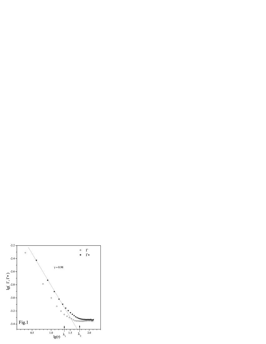
Figure 1 shows the pattern of SDSS galaxy density variations with distance. We can reliably distinguish the main features of the galaxy distribution on various scales. Up to $20h^{-1}$ Mpc, the gamma function is well fitted by a power law with the index (the slope in the logarithmic axes) $\gamma=0.98\pm 0.02$ . On a scale of ( $20-25h^{-1}$ Mpc, significant deviations from a linear dependence begin — the gamma function exhibits a break; the change in the slope is sharper for $\Gamma$ (r), which reflects the change in the state of clustering more accurately than $\Gamma^{*}$ (r), since the latter is more inertial. This suggests that the corresponding changes in the galaxy distribution also occur on a scale of $20h^{-1}$ Mpc abruptly. This effect may be related to the sizes of superclusters. The transition regime of clustering follows next (the density decreases with distance, but more slowly than on the power-law portion) and the distribution of SDSS galaxies becomes homogeneous beginning from a scale of $50-60h^{-1}$ Mpc. The depth of the sample allows spheres up to $130h^{-1}$ Mpc (the scale $R_{s}$ ) to be fitted in its volume and the extent of the ”homogeneous” portion of the density variation with distance is considerable.

It follows from our analysis of volume-limited samples with the angle boundaries $-47^{\circ}<\lambda<8^{\circ}$ and $9^{\circ}<\eta<36^{\circ}$ , different constraints on the radial coordinate ( $z_{max}$ ), and, accordingly, different upper limits on the absolute magnitudes of the galaxies included in the sample (up to the sample with the largest sphere that can be fitted in its boundaries, $\sim 100h^{-1}$ Mpc) that the form of the gamma function described above is stable for galaxies with $r$ -band absolute magnitudes $M_{abs}<-21$ . Our analysis of samples with even lower $z_{max}$ (the radius of the largest sphere is smaller than $100h^{-1}$ Mpc) showed the stability of the presence and scale of the break at $20-25h^{-1}$ Mpc.

To assert that the distribution of galaxies is fractal up to $20h^{-1}$ Mpc, the power law must be observed in a considerably larger interval of scales (McCauley 2002), since inhomogeneous distributions of an arbitrary type can yield a power-law gamma function in a small interval of scales. At the same time, the homogeneity of the galaxy distribution on scales larger than $100h^{-1}$ Iie has been firmly established. The large-scale structure is characterized by the presence of inhomogeneities with an extent of more than $100h^{-1}$ Mpc. For example, the extent of the Sloan Great Wall structure is believed to be more than $300$ Mpc. Therefore, the structuring of the Universe is not limited by the homogeneity scale, but, at the same time, the homogeneity of the distribution is consistent with the presence of structures on scales larger than the homogeneity scale (see, e.g., Gaite et al. 1999).

Thus, the conclusions about the pattern of the distribution of galaxies, clusters, and superclusters reached by Tikhonov et al. (2000) are confirmed completely.

5 THE LUMINOSITY DEPENDENCE OF CLUSTERING

In this paper, we studied the dependence of the slope of the gamma function before the break on the luminosity range of the galaxies included in our volume-limited sample. To study the dependence of the correlation index $\gamma$ over a wide luminosity range, we chose the redshift boundaries $z_{min}=0.03$ and $z_{max}=0.065$ . The upper limit on the absolute magnitude of the galaxies included in our volume-limited sample with these boundaries is $M_{lim}=-19.58$ . We chose the $M_{lim}$ range in which we analyzed the dependence, $-19.6$ (14703 galaxies) — $-21.6$ (1381 galaxies), in such a way that the sample was volume-limited and that a considerable number of galaxies remained in the sample (the number of objects in the sample decreases with decreasing $M_{lim}$ ). In Fig.2, $\gamma$ is plotted against $M_{lim}$ . Since the samples drawn in this way overlap in bright objects, $\gamma$ varies smoothly. The dependence exhibits a break near $M_{lim}=-20.2$ followed by a more rapid increase in $\gamma$ .

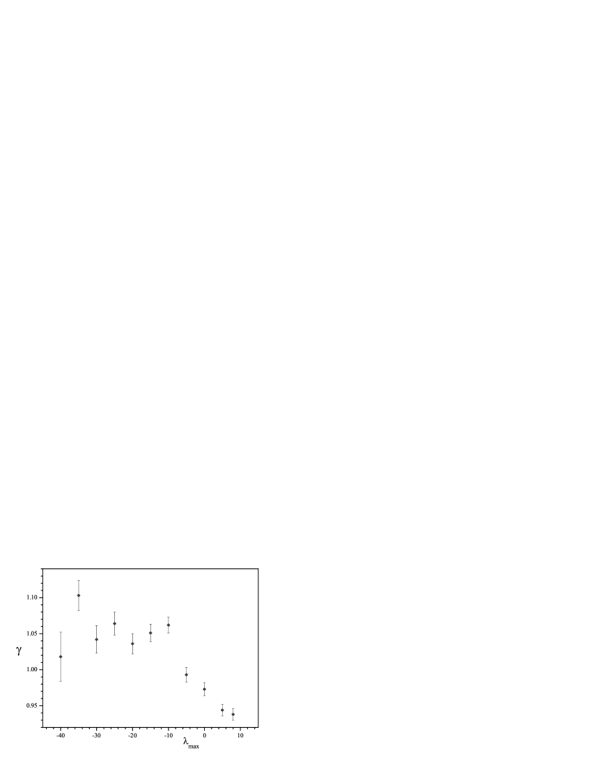
To analyze the possible systematic trends related to the change in the number of objects and in the volume of space covered by the sample, we analyzed the dependence of $\gamma$ on the chosen far boundary (the redshift boundary $z_{max}$ )at fixed $M_{lim}=-21.5$ (Fig.3) and the dependence of $\gamma$ on the longitude sample boundary $\lambda_{max}$ at $\lambda_{min}=-47^{\circ}$ , $z_{max}=0.12$ , and $M_{lim}=-21.5$ (Fig.4). The index $\gamma$ increases as $z_{max}$ increases to $0.1$ . This may be explained by the fact that new significant structures fall into the sample. We can note a slight decrease in $\gamma$ with increasing $\lambda_{max}$ beginning from $\lambda_{max}=-10^{\circ}$ as the volume and the number of galaxies increase.

The dependence of the correlation index $\gamma$ on $M_{abs}$ in Fig.5 was obtained using a sample with the same geometrical boundaries as those in Fig.2, but with galaxies taken from nonoverlapping ranges of absolute magnitudes (the range is 0.2 wide). This increases the statistical significance of the features in the dependence. The number of objects smoothly decreases from 1861 in the range $-19.6<M_{abs}<-19.8$ to 555 at $M_{abs}<-22.0$ ). The main feature of the dependence in Fig.5 is that $\gamma$ increases significantly near the characteristic value of the luminosity function for SDSS galaxies, $M^{*}=-21.38$ (at $H_{0}=65$ km s^-1Mpc^-1)(Blanton et al. 2003), and above.

6 CONCLUSIONS

Thus, as the amount of data obtained as part of the SDSS project increases, it has become possible to directly test the cosmological principle. The homogeneity of the galaxy distribution has passed from a theoretical assumption confirmed by circumstantial evidence (isotropy of the cosmic microwave background, homogeneity of the sky distribution of radio and X-ray sources, etc.) to a strict observational fact, which automatically closes all the inhomogeneous models of cosmological evolution. The mean galaxy density is now a directly measurable quantity.

Our results suggest that the slope before the break in the gamma function on a scale of $\sim 20h^{-1}$ Mpc (the correlation index $\gamma$ ) depends in a complex way on the luminosity and the region of space in which the measurements are made. This casts doubt on the possibility of describing the distribution of galaxies by a single power law (with a single index $\gamma$ ) on short scales.

The significant increase in the correlation index $\gamma$ with decreasing $M_{abs}$ after the break in the luminosity function for SDSS galaxies is indicative of a close relationship between the spatial distribution of galaxies and parameters of the luminosity function for these galaxies. The increase in $\gamma$ with luminosity must be reproduced in model calculations within the framework of the theory of galaxy formation.

7 ACKNOWLEDGMENTS

This work was supported by the Administration of St. Petersburg (grant no. PD05-1.9-117) and the ”Research and Development in Priority Fields of Science and Technology” Federal Program (project no. 02.438.11.7001).

8 REFERENCES

1. Y. Barishev and P. Teerikorpi, astro-ph/0505185, (2005).

2. M. R. Blanton, D. W. Hogg, J. Brinkmann, et al., Astrophys. J. 595, 819 (2003); astro-ph/0210215.

3. P. H. Coleman and L. Pietronero, Phys. Rep. 213, 311 (1992).

4. M. Davis, in Proceedings of the Conference: Critical Dialogues in Cosmology, Princeton, New Jersey, 1996, Ed. N. Turok (World Sci., Singapore, 1997), p. 13.

5. D. J. Eisenstein, J. Annis, J. E. Gunn, et al., Astron. J. 122, 2267 (2001); astro-ph/0108153.

6. J. Gaite, A. Dominguez, and J. Perez-Mercader, Astrophys. J. 522, L5 (1999).

7. C. Hikage, T.Matsubara,Y.Suto, et al., Publ. Astron. Soc. Jpn. 57, 709 (2005); astro-ph/0506194.

8. D.W.Hogg, D.J.Eisenstein, M. R. Blanton, et al., Astrophys. J. 624, 54 (2005); astro-ph/0411197.

9. D. W. Hogg, astro-ph/9905116 (1999).

10. J. L. McCauley, Physica A 309, 183 (2002); astro-ph/9703046.

11. P. J. E. Peebles, The Large-Scale Structure of the Universe (Princeton Univ. Press, Princeton, N.J., 1980; Mir, Moscow, 1983).

12. M. A. Strauss, D. H. Weinberg, R. H. Lupton, et al., Astron. J. 124, 1810 (2002); astro-ph/0206225.

13. F. Sylos Labini, M. Montuori, and L. Pietronero, Phys. Rep. 293, 61 (1998).

14. A. V. Tikhonov, Astrofizika 45, 99 (2002) [Astrophys. 45, 79 (2002)].

15. A. V. Tikhonov, D. I. Makarov, and A. I. Kopylov, Bull. Spwc, Aastrofiz. Obs. 50, 39 (2000); astro-ph/0106276.

16. D.J.York, J. Adelman, J. E. Anderson, etal.,Astron. J. 120, 1579 (2000); astro-ph/0006396.

17. I. Zehavi, Z. Zheng, D. Weinberg, et al., Astrophys. J. 630, 1 (2005); astro-ph/0408569.

Refer to caption — Figure 1: Gamma function of a volume-limited sample of galaxies from the SDSS Main Galaxy Sample with $z_{min}=0.05$ , $z_{max}=0.16$ , $M_{abs}<-21.77$ , $N=18916$ is the number of galaxies in the sample, $R_{s}=132$ Mpc, $\lambda_{1}$ is the break scale, and $\lambda_{2}$ is the homogeneity scale.