Low-Mass Dwarf Template Spectra from the Sloan Digital Sky Survey

Abstract

We present template spectra of low-mass (M0-L0) dwarfs derived from over 4,000 Sloan Digital Sky Survey (SDSS) spectra. These composite spectra are suitable for use as medium-resolution (R $\sim$ 1,800) radial velocity standards. We report mean spectral properties (molecular bandhead strengths, equivalent widths) and use the templates to investigate the effects of magnetic activity and metallicity on the spectroscopic and photometric properties of low-mass stars.

1. Introduction

Low-mass dwarfs are the dominant stellar component of the Galaxy. These ubiquitous stars, with main sequence lifetimes greater than the Hubble time (Laughlin et al., 1997), have been employed in a variety of Galactic studies: tracing Galactic Disk kinematics (Hawley et al., 1996; Gizis et al., 2002; Lépine et al., 2003; Bochanski et al., 2005), describing age-velocity dispersion relations (West et al., 2006), and studying Galactic structure components (Reid et al., 1997; Kerber et al., 2001; Pirzkal et al., 2005). Modelling of their internal structure, atmospheric properties and magnetic activity (Burrows et al., 1993; Baraffe et al., 1998; Allard et al., 1997; Hauschildt et al., 1999; Allred et al., 2006; West et al., 2006) presents interesting theoretical problems. Observationally, the spectra of these stars are marked by the presence of strong molecular absorption features, particularly titanium oxide (TiO), which dominates the optical opacity of their cool atmospheres. The TiO features, along with molecular bandheads introduced by vanadium oxide (VO) and calcium hydride (CaH) are used to define the widely accepted M spectral subtype classification scheme (Kirkpatrick et al., 1991; Reid et al., 1995a; Kirkpatrick et al., 1999).

In order to increase the utility of low-mass stars in large studies of galactic structure and dynamics, we have been engaged in analyzing spectroscopic data from the Sloan Digital Sky Survey (SDSS; York et al., 2000), resulting in a series of papers that describe our methods for photometrically selecting and spectral typing these objects (Hawley et al., 2002; West et al., 2004; Walkowicz et al., 2004; West et al., 2005) and discussing their magnetic activity properties (West et al., 2004, 2006). However, we have been unable to exploit the velocity information contained in the spectra due to the inability of the SDSS pipeline reductions to provide accurate velocites for M dwarfs (Abazajian et al., 2004). Our motivation for the present work is the desire to produce a set of radial velocity templates by combining native, high-quality, SDSS spectra at each spectral subtype in the M dwarf sequence. Additionally, we split the spectra at each subtype into active and inactive stars, and examine the spectroscopic and photometric properties of these templates separately, to determine whether the activity is imprinting a signature that may affect our velocity analysis, and to followup on previous suggestions that colors and detailed absorption features may change depending on activity level (Hawley et al., 1996; Amado & Byrne, 1997; Hawley et al., 1999).

The radial velocity (RV) of an object is the projection of its intrinsic motion onto the line of sight of an observer. In order to accurately determine the RV of a given star, one must carefully address the systematics imposed by the time and location of the observation. This is usually accomplished by shifting the frame of the observer to a heliocentric (sun-centered) or barycentric (center-of-mass centered) rest frame. The standard method of determining stellar and galactic RVs has been cross-correlation, as introduced by Tonry & Davis (1979). This method compares the spectrum of a science target against a known template, using cross-correlation to determine the wavelength shift (and therefore velocity) necessary to align the target with the template. Thus, correlating with a template spectrum that is similar to the science target in all ways except velocity ensures the most accurate determination of the RV.

In the following sections, we report on our efforts to establish a set of low-mass star template spectra suitable for RV analysis using SDSS spectra at medium (R $\sim$ 1,800) resolution. In §2, we describe the observational material from the SDSS and introduce the problems with the RVs reported for low-mass stars by the standard SDSS spectroscopic pipeline. The observations were spectral-typed, inspected for signs of chromospheric activity, and coadded to form templates at each spectral type, as discussed in §3. The resulting spectral templates, their accuracy as RV standards, and their spectral and photometric properties are detailed in §4. Our conclusions follow in §5.

2. Data

2.1. SDSS Photometry

The Sloan Digital Sky Survey (York et al., 2000; Gunn et al., 1998; Fukugita et al., 1996; Hogg et al., 2001; Smith et al., 2002; Stoughton et al., 2002; Abazajian et al., 2003; Pier et al., 2003; Abazajian et al., 2004; Ivezić et al., 2004; Abazajian et al., 2005; Adelman-McCarthy et al., 2006; Gunn et al., 2006) has revolutionized optical astronomy. Centered on the Northern Galactic Cap, SDSS has photometrically imaged $\sim$ 8,000 sq. deg. in five filters ($u,g,r,i,z$) to a faint limit of 22.2 mag in $r$. This has resulted in photometry of $\sim$ 180 million objects with typical photometric uncertainties of $\sim$ 2% at $r\sim 20$ (Ivezić et al., 2003; Adelman-McCarthy et al., 2006). SDSS imaging has been invaluable in recent studies concerning low-mass dwarfs, particularly the colors of the M star sequence (Walkowicz et al., 2004; West et al., 2005) and the study of L and T spectral types (Strauss et al., 1999; Fan et al., 2000; Leggett et al., 2000; Tsvetanov et al., 2000; Hawley et al., 2002; Knapp et al., 2004; Chiu et al., 2006).

2.2. SDSS Spectroscopy

Photometry acquired in SDSS imaging mode is used to select spectroscopic followup targets. The photometry is analyzed by a host of targeting algorithms (originally described in Stoughton et al., 2002) with the primary spectroscopic targets being galaxies (Strauss et al., 2002), luminous red galaxies with z $\sim 0.5-1.0$ (Eisenstein et al., 2001), and high redshift quasars (Richards et al., 2002). Designed to acquire redshifts for $\sim$ 1,000,000 galaxies and 100,000 quasars, twin fiber-fed spectrographs deliver 640 flux-calibrated spectra per 3^∘ diameter plate over a wavelength range of 3800-9200Å with a resolution $R\approx$ 1,800. Typical observations are the coadded result of multiple 15 minute exposures, with observations continuing until the signal-to-noise ratio per pixel is $>$ 4 at $g=20.2$ and $i=19.9$ (Stoughton et al., 2002). Typically, this takes about 3 exposures. Wavelength calibrations, good to 5 km s^-1 or better (Adelman-McCarthy et al., 2006), are carried out as described in Stoughton et al. (2002). The spectra are then flux-calibrated using F subdwarf standards, with broadband uncertainties of 4% (Abazajian et al., 2004). These observations, obtained and reduced in a uniform manner, form a homogeneous, statistically robust dataset of over 673,000 spectra (Adelman-McCarthy et al., 2006). SDSS has already proven to be an excellent source of low-mass stellar spectroscopy (Hawley et al., 2002; Raymond et al., 2003; West et al., 2004; Silvestri et al., 2006). Unfortunately, the RVs determined for low-mass stars in the SDSS pipeline are known to be inaccurate(Abazajian et al., 2004). These systematic errors, on the order of 10 km s^-1 (Abazajian et al., 2004) result primarily from spectral mismatch, since there are only four low-mass stellar templates in the standard spectroscopic pipeline. Thus, we sought to remedy this situation by establishing a uniform set of low-mass RV templates derived from SDSS spectroscopy.

3. Analysis

To build a database of low-mass stellar spectra, we queried the Data Release 3 (DR3; Abazajian et al., 2005) Catalog Archive Server (CAS) for spectra with late-type dwarf colors (from West et al., 2005), using $0.5<r-i<3.05$ and $0.3<i-z<1.9$. The color ranges quoted in West et al. (2005) were slightly extended to increase the total number of low-mass stellar spectra. These color cuts were the only restrictions applied to the DR3 data. We treated each spectral subtype independently, performing 11 (M0-L0) queries, some of which overlapped in color-color space (see Table 1). Thus, some spectra were selected twice, usually in neighboring spectral subtypes (i.e., M0 and M1). These queries yielded $\sim$ 133,000 candidate spectra in the 11 (M0-L0) spectral type bins.

3.1. Spectral Types and Activity

The candidate spectra were examined with a suite of software specifically designed to analyze M dwarf spectra. This pipeline, as introduced in Hawley et al. (2002), measures a host of molecular band indices (TiO2, TiO3, TiO4, TiO5, TiO8, CaH1, CaH2, and CaH3), and employs relations first described by Reid et al. (1995a) to determine a spectral type from the strength of the TiO5 bandhead. All spectral types were confirmed by manual inspection, adjusting the final spectral type, if necessary. The accuracy of the final spectral type is $\pm 1$ subtype. Additionally, the software pipeline measures the equivalent width (EW) of the H$\alpha$ line, quantifying the level of magnetic activity in a given low-mass dwarf. See West et al. (2004) for details on the measurement of bandheads and line strengths in low-mass star SDSS spectra.

Inspection of each candidate spectrum allowed us to remove contaminants (mostly galaxies) from the sample, reducing its size to $\sim$20,000 stellar spectra. We also removed the white dwarf-M dwarf pairs that were photometrically identified by Smolčić et al. (2004). The database was then culled of duplicates. As shown in West et al. (2005) (and Table 1), M dwarfs of different spectral types can possess similar SDSS photometric colors. Thus, some spectra with overlapping photometric colors were duplicated in our original database (see §3 and Table 1). Each duplicate spectrum was identified by filename and in cases where different spectral types were manually assigned by eye to the same star (typically one subtype apart), the earlier spectral type was kept. The typical difference in spectral type was one subclass, in agreement with our stated accuracy. These various cuts reduced the sample from $\sim$20,000 to $\sim$12,000 stars.

The spectra were then categorized based on their activity. In order to be considered active, a star had to meet the criteria originally described in West et al. (2004): (1) The measured H$\alpha$ EW is larger than 1.0 Å; (2) The measured EW is larger than the error; (3) The height of the H$\alpha$ line must be three times the noise at line center; (4) The measured EW must be larger than the average EW in two 50 Å comparison regions (6500-6550 Å and 6575-6625 Å). In order to be considered inactive, the measured EW had to be less than 1.0 Å  and have a signal-to-noise ratio greater than three in the comparison regions. By selecting only these active and inactive stars, our final sample is limited to spectra with well-measured features, removing spectra with low signal-to-noise ratios. The resulting database consisted of $\sim$6,000 stellar spectra.

3.2. Coaddition

SDSS spectra are corrected to a heliocentric rest frame during the standard pipeline reduction and are on a vacuum wavelength scale. To assemble the fiducial template spectra, stars of a given spectral type were first shifted to a zero-velocity rest frame, then normalized and coadded. Multiple strong spectral lines were used to measure the velocity of each star to obtain an accurate shift to the rest frame. For inactive stars, the red line (7699 Å) of the K I doublet and both lines of the Na I doublet (8183, 8195 Å) were measured, while in active stars, H$\alpha$ was also used. These spectral line combinations were selected for their strength in all low-mass stellar spectra, ensuring that no single line would determine the final velocity of a star. Spectral lines were fit with single Gaussians and inspected visually to ensure proper fitting. Stars with spurious fits or discrepant line velocities (lines which deviated from the mean by $>$ 30 km s^-1) were removed from the final coaddition. Removing these spectra reduced the final sample size to $\sim$ 4,300 stars. The classical redshift correction was then applied to each spectrum in the final sample, justifying them to a zero-velocity rest frame.

The velocity of each spectral line in the final sample was fit with an measurement uncertainty of $\sim$ 10 km s^-1, as determined by the mean scatter among individual line RV measurements. In wavelength space, this translates to about 0.2 Å resolution near H$\alpha$ (note the resolution of SDSS (R $\sim$ 1,800) implies 3.6 Å resolution at H$\alpha$). Since the observed spectrum is a discretization of a continuous flux source (i.e., the star), wavelength shifts introduced by the radial velocity of a star will move flux within and between resolution elements. These wavelength shifts, which are resolved to subpixel accuracy, act to increase the resolution of the final co-added spectrum (see Pernechele et al., 1996). This is similar to the common “drizzle” technique of using multiple, spatially distinct low-resolution images to produce a single high-resolution image (Fruchter & Hook, 2002).

The wavelength-justified spectra were then normalized at 8350Å and coadded (with equal weighting of each spectrum) using the following prescription. At each subtype, we attempted to construct three templates: one composed solely of active stars (Fig. 1), one composed of inactive stars (Fig. 2), and a third composed of both the inactive and active stars from the previous two sets (Fig 3). For each template, the mean and standard deviation were calculated at each pixel. In later ($>$ M7) subtypes, the lack of spectra meeting our activity and velocity criteria resulted in fewer templates.

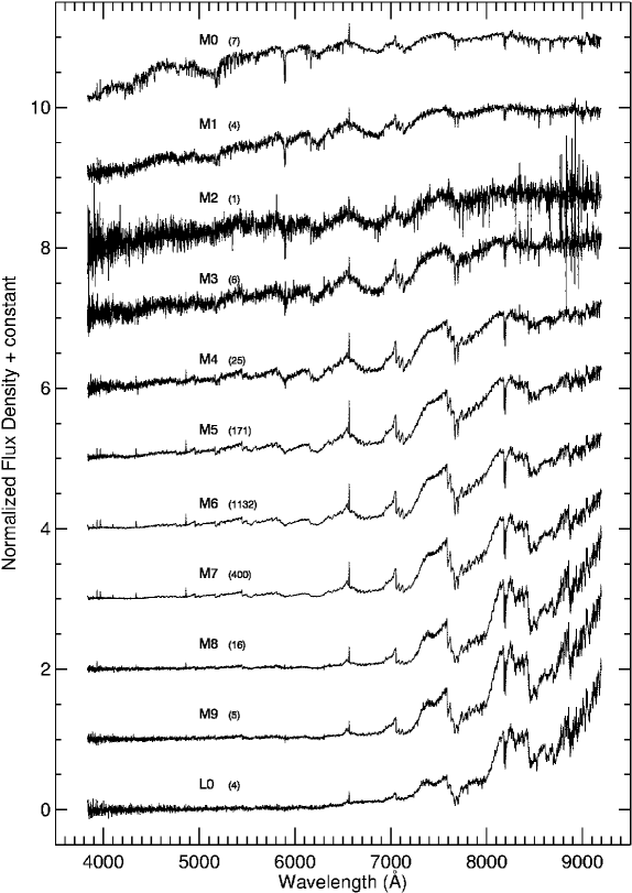
Figure 1.— Mean template spectra of active low-mass dwarfs of types M0-L0. The spectral type and number of stars (in parentheses) are labeled for each template.

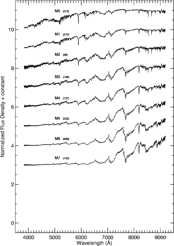
Figure 2.— Mean template spectra of inactive low-mass dwarfs of types M0-M7. No M8-L0 dwarfs met the activity and consistent line velocity criteria. Spectral type and number of stars in each template are labeled.

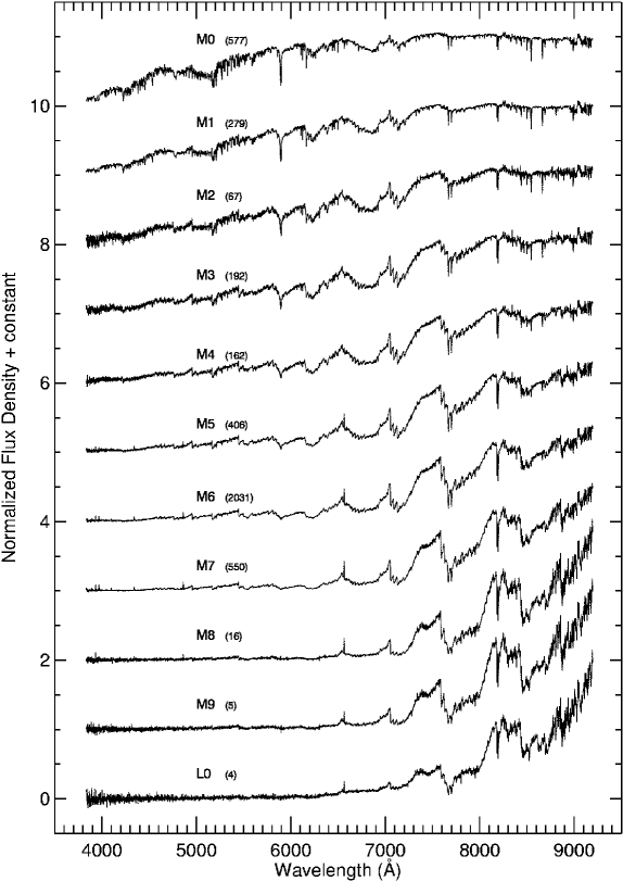
Figure 3.— Mean composite template spectra for low-mass dwarfs of types M0-L0, formed by combining the data shown in Figures 1 and 2. Spectral type and number of stars in each template are labeled.

4. Results and Discussion

The final template spectra (Figures 1-3) represent the mean spectral properties of low-mass dwarfs as observed by the SDSS spectrographs. In Figure 4, we show illustrative examples of our templates for an inactive M1 star and an active M6 star, with strong atomic lines and molecular bandheads labeled. Prominent molecules include MgH, CaH, TiO, VO and CaOH. The active stars show the Balmer series to H8 ($\lambda\sim$ 3889 Å) along with Ca II H and K ($\lambda\sim$ 3968, 3933 Å). In Figure 5 we compare a high signal-to-noise SDSS spectrum of an M5 star to its template counterpart in the region near H$\alpha$. It is clear that the template has significantly higher spectral resolution; e.g. a weak feature near 6575 Å is visible only in the template. In the following sections, we explore the feasibility of using these templates as RV standards and the effects of chromospheric activity and metallicity on the mean spectroscopic and photometric characteristics of low-mass stars.

4.1. Radial Velocity Accuracy

The primary uncertainties associated with determining RVs using the cross-correlation method are due to the resolution of the spectra, accuracy of the wavelength calibration and matching the spectral type of the template and science data. To ensure that the RVs measured with our templates are accurate, we have carried out tests that quantify the internal consistency and external zero-point precision of these templates. These tests are described below.

4.1.1 Internal Consistency

To quantify the internal consistency among templates, sequential spectral types were cross-correlated using the $fxcor$ task in IRAF. This minimizes the error introduced by spectral type mismatch, which often dominates the errors associated with cross-correlation redshift measurements (Tonry & Davis, 1979). Thus, wavelength calibration and intrinsic resolution are the major sources of uncertainty in our analysis. In all cases (i.e., active, inactive and combined templates) the mean difference in velocity between adjacent spectral subtypes was $\lesssim$ 1 km s^-1. This compares favorably with the 3.5 km s^-1 spread in SDSS data as reported by York et al. (2000). Note this value is derived from observations of stars in M67 (Mathieu et al., 1986), and does not include any low-mass dwarfs.

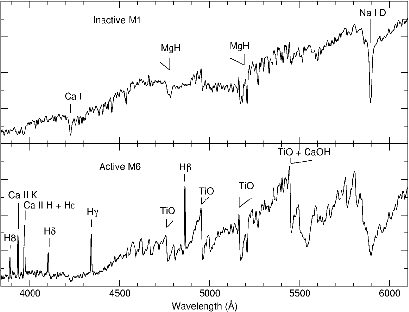
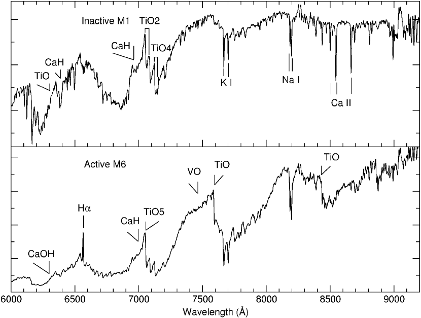
Figure 4.— Illustrative template spectra of an inactive M1 star and an active M6 star with strong molecular and atomic features labeled.

Figure 5.— Comparison of a high signal-to-noise SDSS M5 spectrum (bottom) to the active M5 template (top) near H$\alpha$. Note the higher resolution of the template spectrum.

4.1.2 External Consistency: Hyades

To test the external accuracy of the template spectra, they were cross-correlated against Hyades cluster members with well-measured RVs, observed as part of our SDSS collaboration effort to produce RV standards for low-mass dwarfs. Each Hyades star has a known RV (Reid & Mahoney, 2000; Stauffer et al., 1994, 1997; Terndrup et al., 2000; Griffin et al., 1988) or is a confirmed member of the cluster, whose dispersion is $<$ 1 km s^-1 (Gunn et al., 1988; Makarov et al., 2000). The Hyades RVs in the literature were measured from high-resolution echelle spectra, with a typical accuracy of $\lesssim$ 1 km s^-1. Thus, the SDSS spectra of these Hyads provide a way to check our cross-correlation RVs against an external standard system.

The medium-resolution spectra of the Hyades stars secured by SDSS were correlated against our templates, with results shown in Figure 6. The high-resolution echelle data have a mean of 38.8 km s^-1 and a standard deviation of 0.27 km s^-1. The RVs measured with our template spectra yield a mean RV of 42.6 km s^-1 with a standard deviation of 3.2 km s^-1. By comparison, the SDSS pipeline RVs produced a mean velocity of 31.9 km s^-1 and a standard deviation of 6.8 km s^-1 (after removing two highly discrepant measurements). Using the template spectra better reproduces the coherent velocity signature of the Hyades and provides much more reliable velocities than the standard SDSS pipeline measurements. The templates are therefore well-suited for use as medium-resolution RV standards for low-mass dwarfs.

Figure 6.— Histogram comparison of high-resolution echelle RV measurements (solid line), medium resolution cross-correlation RV determinations (dashed line), and SDSS pipeline RVs (dotted line) for 19 Hyades M dwarfs. Note the SDSS pipeline reported wildly discrepant velocities for two stars (not shown).

4.2. Spectral Differences: Activity & Metallicity

The effect of magnetic activity on the spectral properties of a low-mass star is clearly manifested by the existence of emission lines. This effect is often quantified by measuring the luminosity in the H$\alpha$ line divided by the bolometric luminosity ($L_{\rm H\alpha}/L_{\rm Bol}$). Other changes due to activity, such as varying strength of molecular bandheads (Hawley et al., 1996, 1999) and changes in the shape of the continuum have been sparsely investigated. Additionally, metallicity affects the strength of molecular bandheads at a given temperature (see Woolf & Wallerstein, 2006). Using the template spectra as fiducial examples of thin-disk, solar-metallicity low-mass stars, we next examine changes in the spectral properties of low-mass stars introduced by magnetic activity and metallicity.

4.2.1 Activity: Decrements & $L_{\rm H\alpha}/L_{\rm Bol}$

Emission features are dependent on the temperature and density structure of the outer stellar atmosphere. The line fluxes of the Balmer series lines and the Ca II K line ($\lambda\sim 3933$ Å) can be used to examine the structure of the chromosphere in magnetically active stars (Reid et al., 1995b; Rauscher & Marcy, 2006) and to investigate chromospheric heating in quiescent (i.e. non-flaring) dMe stars (Mauas & Falchi, 1994; Mauas et al., 1997). The Balmer decrement (ratios of Balmer line strengths to a fiducial, here taken to be H$\beta$) is traditionally used to quantify medium-resolution spectra. Table 2 gives the Balmer series and Ca II K decrements for the active templates. There is no strong trend in the decrement with spectral type for the template spectra, which is consistent with the previous study of Pettersen & Hawley (1989), who reported average decrements over a range of K and M spectral types. However, both the templates and Pettersen & Hawley (1989) show a gradual increase in the H$\alpha/$H$\beta$ ratio with spectral type (see Table 2). Evidently the structure and heating of low-mass stellar chromospheres remains fairly similar over the range of M dwarf effective temperature (mass), with the H$\alpha$ gradually becoming stronger relative to the higher order Balmer lines at later spectral type.

The Balmer decrements observed in AD Leo (dM3e) during a large flare (Hawley & Pettersen, 1991) and determined for quiescent and flaring model atmospheres (Allred et al., 2006) are given in Table 2 for comparison. In Figure 7, we plot these observed and model decrements together with the average Balmer decrements of the active low-mass stellar templates. The flare decrements, both observed and model, are much flatter than those in the non-flaring atmospheres, suggesting (though within the errors) increased emission in the higher order Balmer lines. This probably reflects the higher chromospheric densities (hence greater optical depth in the Balmer line-forming region) in the flare atmospheres. Evidently the range in chromospheric properties among M dwarfs of different spectral types is much less (during quiescent periods) than in a given star between its quiet and flaring behavior.

For completeness, the average Balmer line and Ca II K EWs and the quantity $L_{\rm H\alpha}/L_{\rm Bol}$ measured from the active templates are reported in Table 3. $L_{\rm H\alpha}/L_{\rm Bol}$ which is used to quantify activity, was calculated using the H$\alpha$ EW and the ($i-z$) continuum ($\chi$) relation of West et al. (2005), as first described in Walkowicz et al. (2004). The average EWs reported in Table 3 agree with previous results (Stauffer et al., 1997; Gizis et al., 2002). The general increase toward later types is attributed to the lower continuum flux in the vicinity of H$\alpha$ as the stellar effective temperature decreases. The $L_{\rm H\alpha}/L_{\rm Bol}$ ratios are also consistent with previous studies (Hawley et al., 1996; Gizis et al., 2000; West et al., 2004), attaining a relatively constant value (with large scatter) among early-mid M (M0-M5) types, and decreasing at later types.

Figure 7.— Decrements for the averaged active templates (open diamonds, error bars) are shown. Also shown are results for the dM3e star AD Leo: observed flare (filled circles; from Hawley & Pettersen, 1991), model flare (open squares), and model quiescent (open triangles) decrements (Allred et al., 2006). Flaring atmospheres have increased density at chromospheric temperatures, resulting in higher opacity and increased emission in the higher-order Balmer lines compared to H$\alpha$. The result is a relatively flatter decrement.

4.2.2 Activity: Bandheads

Molecular rotational and vibrational transitions imprint large bandheads on the observed spectra of low-mass stars. The strength of the TiO bandheads in the visible is often used as a spectral-type discriminant (Reid et al., 1995a). Additionally, CaOH, TiO and CaH bandheads have been employed as temperature and metallicity indicators (Gizis, 1997; Hawley et al., 1999; Woolf & Wallerstein, 2006). Following previous conventions (Reid et al., 1995a; Kirkpatrick et al., 1999), we provide measurements for the CaH bandheads at $\sim$ 6400Å (CaH1), $\sim$ 6800Å (CaH2,CaH3) in Table 4, and for the TiO bandheads at $\sim$ 7050Å (TiO2,TiO4,TiO5) and $\sim$ 8430Å (TiO8) in Table 5. Note that TiO2 and TiO4 are sub-bands of the full TiO5 bandhead.

As first observed by Hawley et al. (1996), activity can introduce changes in the TiO bandheads (Hawley et al., 1999; Martín, 1999). Shown in Figure 8 is the TiO2 index as a function of the TiO4 index. For active stars, the strength of the TiO2 bandhead is increased (smaller index) at a given value of the TiO4 index. Alternately, at a given index of TiO2, the TiO4 index is weaker in active stars. This provides interesting constraints on the structure of the atmosphere, suggesting that the formation of TiO, thought to take place near the temperature minimum region below the chromospheric temperature rise (Chabrier et al., 2005; Reid & Hawley, 2005), is affected by the presence of an overlying chromosphere. The opposite behavior of these two sub-bands serves to decrease the sensitivity of TiO5 to chromospheric activity, making it a good temperature (spectral-type) proxy regardless of the activity level of the star (see Hawley et al., 1999).

Figure 8.— TiO2 vs. TiO4 for active (open triangles) and inactive (filled circles) templates. At a constant TiO4 value, TiO2 is deeper (smaller index values) in the active stars, confirming the result originally discussed in Hawley et al. (1996).

4.2.3 Activity: Spectral Features

Two main effects influence the colors of active stars: the presence of emission lines and changes in the continuum emission. To investigate these effects, we divided the active templates by their inactive counterparts. Figure 9 is an illustrative example of our analysis, showing the individual active and inactive M0 template spectra together with the ratio of the active to inactive flux. The approximate wavelength bounds of the SDSS $g,r$ and $i$ filters are indicated. The ratio shows enhanced blue continuum emission in the active template, and significantly enhanced emission lines, particularly in Ca II H and K. These effects lead to a bluer ($g-r$) color for the active star (see Table 6, discussed further in §4.3 below). The change in color is dominated by the continuum enhancement, with the increased emission line flux providing only a marginal effect. Similar continuum and line flux enhancements are observed during flares, suggesting that the active M0 template may include one or more stellar spectra obtained during low level flaring conditions. As described in Güdel et al. (2002), low level flaring maybe responsible for a significant fraction of the “quiescent” chromospheric emission observed on active stars.

The ratio also shows two “emission” lines in the $r$ band corresponding to emission in the core of the Na I D doublet ($\lambda\sim$5900 Å, doublet marginally resolved at SDSS resolution, but well resolved in our templates) and in H$\alpha$. Again, these lines do not significantly contribute to the combined flux of the template in the $r$ band, as shown by the marginally redder $r-i$ color for the active template in Table 6. The spectral flux ratio in the $i$ band is very close to unity, with no strongly varying emission or continuum features between the active and inactive templates. This analysis suggests that changes in the continuum emission of active stars provide the most important contribution to observed color differences.

The variable strength of the CaOH (6230 Å) bandhead is also of note. Shown in Figure 10 are the active to inactive ratios for M4-M7 subtypes. The growth of this feature indicates there is some dependence of the formation mechanism of CaOH on spectral type (effective temperature, mass), perhaps changing the position of the temperature minimum within the atmosphere. Note that the feature near this wavelength previously discussed as a good temperature indicator by Hawley et al. (1999) is actually due to TiO in early M dwarfs. CaOH begins to dominate the opacity in this region only at types later than M4, which were not available to observation in the clusters described by Hawley et al. (1999). Therefore these new SDSS observations are the first evidence of a real effect in the CaOH band that differs with the presence of a chromosphere and changes with spectral type. These observations, together with the differences in the TiO2 and TiO4 bands should provide strong constraints on the next generation of atmospheric models (including chromospheres) for M dwarfs.

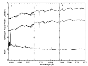
Figure 9.— Shown is an illustrative example of our flux-ratio analysis. The active M0 spectral template (top) is divided by the inactive (middle) template. The resulting flux ratio is plotted on the bottom. The windows display the approximate wavelength bounds of the SDSS $g$,$r$, and $i$ filters.

Figure 10.— The ratio of the active to inactive flux for the M4-M7 templates is shown in the vicinity of the CaOH (6230 Å) bandhead. Note the increase in the ratio at later types, indicating a shallower CaOH band in the active template compared to its inactive counterpart. Apparently, the formation mechanism of CaOH depends on both the star’s spectral type (effective temperature) and the presence of a chromosphere.

4.2.4 Metallicity: Spectral Features

We explored the effects of metallicity on the spectra by comparing our composite templates to a low-metallicity subdwarf ([Fe/H] $\sim-0.5$; Woolf & Wallerstein, 2006) and a metal-rich Hyades dwarf ([Fe/H] = 0.13, Paulson et al., 2003) , both observed with SDSS. The results are shown in Figure 11. Previous studies (West et al., 2004) indicate that subdwarfs are $\sim$ 0.2 mags redder than solar-metallicity stars in $g-r$. This is most likely due to the multiple hydride bands present in the $g$ filter (Hartwick, 1977; Dahn et al., 1995; West et al., 2004). The region between 4000-4500Å in Figure 11 (left panel) shows that the flux in the subdwarf is depressed by $\sim$ 60% compared to the level present in the composite template. Strong hydride bands, such as MgH near 5000Å and CaH bands near 6800Å are also depressed. These bands are labeled in Figure 4.

In contrast, the metal-rich Hyades star (right panel of Fig. 11) shows mostly enhanced but variable continuum in the $g$ band, which is difficult to attribute to any particular feature. There is enhanced emission in the core of Na I D and Ca II H and K, but these are likely not strong enough to influence the colors. Unfortunately we do not have colors in the SDSS filters, measured with the 2.5m SDSS telescope, for the Hyades stars, and therefore cannot directly compare the spectral features with measured color differences between the metal-rich stars and our templates.

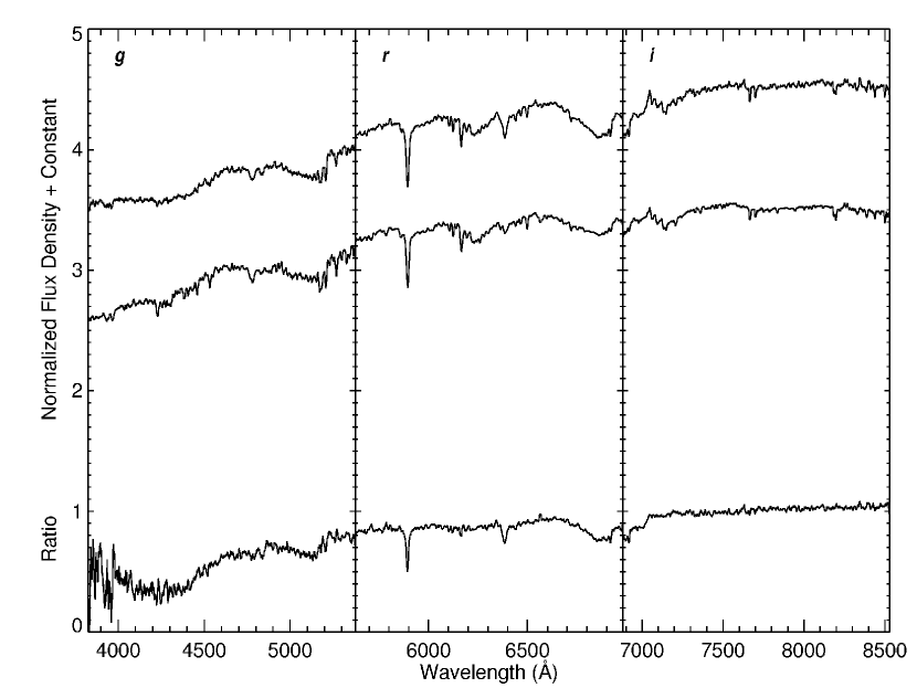
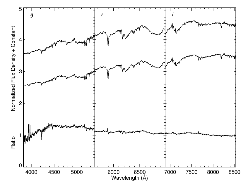
Figure 11.— Shown are illustrative examples of our flux ratio analysis of an M0 subdwarf (left panel) and an M1 Hyades star (right panel). The subdwarf and Hyades star are the top spectra in their respective panels; the composite template of the same spectral type (from Figure 3) appears as the middle spectrum, and the ratio of the two spectra is shown on the bottom.

4.3. Photometric Differences: Colors

Photometry was obtained from the SDSS CAS for each star used in constructing the templates. The average colors for each template are listed in Table 6 by spectral type. Previous studies have been inconclusive, suggesting that active stars are marginally bluer in $U-B$ (Amado & Byrne, 1997), redder in $V-I$ (Hawley et al., 1999) or not statistically different from inactive populations for SDSS colors (West et al., 2004). We computed the color difference for each spectral subtype (active color - inactive color) and averaged over spectral type. The data in Table 6 indicate the following general trends: active stars are $\sim 0.09\pm 0.24$ mags bluer than their non-active counterparts in $u-g$, while they are $\sim 0.05\pm 0.03$ mags redder in $i-z$. We note that while these trends are suggestive, but are within the scatter. No strong trends were present in $g-r$ or $r-i$.

Our goal was to link changes in the spectral features to differences in photometric colors. Due to the spectral coverage of the SDSS spectra, we are only able to investigate the $g-r$ and $r-i$ colors in detail, which did not demonstrate any discernible trends with activity. The bluer $g-r$ color in the M0 active template appears to be anomalous, and from the spectral analysis, may be due to low level flaring - see §4.2.3. This may also be simply due to the small number of spectra associated with the active M0 template. However, the photometric trend in $u-g$, where active stars were an average of $\sim$ 0.09 mags bluer than inactive stars, may be reflecting the presence of similar low level flaring in many of the active templates, as the enhanced blue continuum during flares will appear even more strongly in the $u$ band (Moffett & Bopp, 1976; Hawley & Pettersen, 1991).

The small number of M subdwarfs identified in the SDSS database, and the lack of SDSS photometry for the Hyades M dwarfs prevented us from investigating color differences due to metallicity. As noted in the previous section, West et al. (2004) showed that M subdwarfs are $\sim$ 0.2 mags redder in $g-r$ than their solar-metallicity counterparts.

5. Conclusions

We used the large SDSS spectral database from DR3 to form active, inactive and composite template spectra of M dwarfs spanning types M0-L0, on a uniform, zero-velocity scale. Our spectral templates provide suitable radial velocity standards for analyzing spectra with R$\sim$ 1,800, with an external accuracy of 3.8 km s^-1, within the quoted error associated with the wavelength scale for SDSS spectroscopy (York et al., 2000). Internally, the templates are consistent to $<$ 1 km s^-1.

The magnetically active templates, as identified by the presence of H$\alpha$ emission in the individual stellar spectra, showed little difference in the measured Balmer decrements with spectral type, indicating that chromospheric structure and heating are apparently similar through the M dwarf sequence. Flares cause much larger changes in the decrement. We found some evidence that color changes (active stars appearing bluer in $u-g$ and in one case in $g-r$) are due primarily to blue continuum enhancements in the active stars, which may be due to intermittent low-level flaring. In general, chromospheric line emission has a negligible effect on the colors of active stars. Molecular bands including TiO2, TiO4 and CaOH showed significant changes between the active and inactive templates.

With regard to metallicity, our findings extend the earlier study by West et al. (2004), which found subdwarfs to be $\sim$ 0.2 mags redder in $g-r$. Our spectral analysis shows that the flux in the blue is depressed by as much as 60%, and that the strong MgH and CaH bands are significantly deeper in the subdwarfs. The spectral analysis of metal-rich Hyades stars ([Fe/H] = 0.13, Paulson et al., 2003) showed continuum differences, but these were not obviously attributed to any particular features.

The authors would like to thank Andrew Becker and Kelle Cruz for their enlightening conversations. The authors gratefully acknowledge the support of NSF grant AST02-05875 and NASA ADP grant NAG5-13111. This research has made use of NASA’s Astrophysics Data System Abstract Service, the SIMBAD database, operated at CDS, Strasbourg, France. This project made extensive use of SDSS data. Funding for the SDSS and SDSS-II has been provided by the Alfred P. Sloan Foundation, the Participating Institutions, the National Science Foundation, the U.S. Department of Energy, the National Aeronautics and Space Administration, the Japanese Monbukagakusho, the Max Planck Society, and the Higher Education Funding Council for England. The SDSS Web Site is http://www.sdss.org/.

The SDSS is managed by the Astrophysical Research Consortium for the Participating Institutions. The Participating Institutions are the American Museum of Natural History, Astrophysical Institute Potsdam, University of Basel, Cambridge University, Case Western Reserve University, University of Chicago, Drexel University, Fermilab, the Institute for Advanced Study, the Japan Participation Group, Johns Hopkins University, the Joint Institute for Nuclear Astrophysics, the Kavli Institute for Particle Astrophysics and Cosmology, the Korean Scientist Group, the Chinese Academy of Sciences (LAMOST), Los Alamos National Laboratory, the Max-Planck-Institute for Astronomy (MPIA), the Max-Planck-Institute for Astrophysics (MPA), New Mexico State University, Ohio State University, University of Pittsburgh, University of Portsmouth, Princeton University, the United States Naval Observatory, and the University of Washington.

Table 1DAS Query Color Ranges

Sp. Type	$r-i$	$i-z$
M0	0.50 - 0.85	0.30 - 0.50
M1	0.60 - 1.15	0.30 - 0.65
M2	0.80 - 1.30	0.40 - 0.75
M3	0.90 - 1.50	0.40 - 0.90
M4	1.10 - 1.80	0.60 - 1.10
M5	1.45 - 2.20	0.80 - 1.15
M6	1.65 - 2.25	0.90 - 1.20
M7	1.90 - 2.70	0.95 - 1.65
M8	2.65 - 2.85	1.20 - 1.90
M9	2.85 - 3.05	1.25 - 1.80
L0	2.30 - 2.70	1.70 - 1.90

Table 2Active Template Decrements

Sp. Type	H$\alpha$	H$\beta$	H$\gamma$	H$\delta$	H$8$	Ca II K
M0	2.09 (0.22)	1.00 (0.15)	$\cdots$	$\cdots$	$\cdots$	$\cdots$
M1	2.33 (0.50)	1.00 (0.28)	$\cdots$	$\cdots$	$\cdots$	0.19 (0.16)
M2	$\cdots$	$\cdots$	$\cdots$	$\cdots$	$\cdots$	$\cdots$
M3	3.08 (0.73)	1.00 (0.28)	$\cdots$	$\cdots$	$\cdots$	$\cdots$
M4	3.37 (0.67)	1.00 (0.26)	0.51 (0.26)	0.43 (0.25)	$\cdots$	$\cdots$
M5	4.27 (1.33)	1.00 (0.34)	1.12 (0.41)	0.52 (0.30)	0.13 (0.36)	0.86 (0.38)
M6	3.68 (0.66)	1.00 (0.24)	0.76 (0.25)	0.36 (0.22)	0.31 (0.33)	0.67 (0.27)
M7	4.18 (0.71)	1.00 (0.23)	0.72 (0.23)	0.47 (0.23)	0.25 (0.32)	0.80 (0.27)
M8	5.90 (1.11)	1.00 (0.25)	0.90 (0.28)	0.64 (0.28)	0.32 (0.39)	$\cdots$
M9	$\cdots$	$\cdots$	$\cdots$	$\cdots$	$\cdots$	$\cdots$
L0	$\cdots$	$\cdots$	$\cdots$	$\cdots$	$\cdots$	$\cdots$
Average	3.61 (1.21)	1.00 (0.00)	0.80 (0.23)	0.48 (0.11)	0.25 (0.09)	0.78 (0.10)
AD Leo (Hawley & Pettersen, 1991)	$\cdots$	1.00	0.81	0.69	0.50	0.18
Quiet Model (Allred et al., 2006)	2.20	1.00	0.58	0.21	0.34	3.65
Flare Model (Allred et al., 2006)	0.57	1.00	0.84	0.75	0.54	0.10

Note. — Decrement measurements are reported with measurement errors in parentheses.

Table 3Active Template Equivalent Widths and $L_{\rm H\alpha}/L_{\rm bol,{\it i-z}}$

Sp. Type	H$\alpha$ EW	H$\beta$ EW	H$\gamma$ EW	H$\delta$ EW	H$8$ EW	Ca II K EW	$L_{\rm H\alpha}/L_{\rm bol,{\it i-z}}$
M0	1.39 (0.04)	1.09 (0.11)	$\cdots$	$\cdots$	$\cdots$	$\cdots$	2.15E-04 (5.48E-05)
M1	1.33 (0.10)	1.54 (0.31)	$\cdots$	$\cdots$	$\cdots$	1.03 (0.84)	1.28E-04 (5.83E-05)
M2	3.57 (0.10)	$\cdots$	$\cdots$	$\cdots$	$\cdots$	$\cdots$	3.24E-04 (2.87E-05)
M3	2.45 (0.31)	2.40 (0.48)	$\cdots$	$\cdots$	$\cdots$	$\cdots$	1.42E-04 (7.00E-05)
M4	4.12 (0.35)	5.10 (0.93)	6.33 (3.09)	7.17 (4.09)	$\cdots$	$\cdots$	1.75E-04 (6.08E-05)
M5	5.85 (1.16)	5.56 (1.34)	16.15 (4.56)	8.28 (4.41)	3.78 (10.26)	25.09 (12.75)	1.82E-04 (7.14E-05)
M6	6.06 (0.39)	7.94 (1.34)	18.88 (5.55)	9.36 (5.75)	9.26 (10.20)	19.10 (9.16)	1.35E-04 (2.43E-05)
M7	8.15 (0.50)	10.47 (1.70)	25.85 (7.89)	15.73 (7.64)	10.29 (13.44)	21.30 (8.84)	1.01E-04 (3.45E-05)
M8	10.99 (0.64)	12.23 (2.24)	113.05 (60.46)	38.65 (19.74)	20.34 (27.37)	$\cdots$	4.41E-05 (1.14E-05)
M9	6.10 (0.18)	$\cdots$	$\cdots$	$\cdots$	10.94 (14.52)	$\cdots$	2.52E-05 (6.41E-06)
L0	6.86 (0.41)	$\cdots$	$\cdots$	$\cdots$	$\cdots$	$\cdots$	1.97E-05 (2.50E-06)

Note. — Equivalent Widths are reported in Åwith measurement errors in parentheses.

$L_{\rm H\alpha}/L_{\rm bol,{\it i-z}}$ measurement errors are also in parentheses.

Table 4Template Bandheads

Sp. Type	CaH1			CaH2			CaH3
	Active	Inactive	All	Active	Inactive	All	Active	Inactive	All
M0	0.94 (0.00)	0.91 (0.01)	0.91 (0.01)	0.79 (0.00)	0.79 (0.01)	0.79 (0.01)	0.87 (0.00)	0.89 (0.01)	0.89 (0.01)
M1	0.86 (0.01)	0.85 (0.02)	0.85 (0.02)	0.68 (0.01)	0.67 (0.01)	0.67 (0.01)	0.82 (0.01)	0.83 (0.02)	0.83 (0.02)
M2	0.81 (0.01)	0.80 (0.03)	0.80 (0.03)	0.49 (0.01)	0.56 (0.03)	0.56 (0.03)	0.68 (0.01)	0.76 (0.04)	0.76 (0.04)
M3	0.74 (0.04)	0.78 (0.07)	0.78 (0.07)	0.48 (0.03)	0.48 (0.06)	0.48 (0.06)	0.71 (0.04)	0.72 (0.09)	0.72 (0.09)
M4	0.76 (0.03)	0.76 (0.04)	0.76 (0.04)	0.39 (0.02)	0.43 (0.02)	0.42 (0.02)	0.65 (0.03)	0.69 (0.04)	0.68 (0.04)
M5	0.75 (0.04)	0.80 (0.03)	0.78 (0.04)	0.37 (0.03)	0.38 (0.02)	0.38 (0.02)	0.64 (0.04)	0.67 (0.03)	0.66 (0.04)
M6	0.76 (0.03)	0.79 (0.07)	0.77 (0.05)	0.33 (0.01)	0.33 (0.03)	0.33 (0.02)	0.60 (0.02)	0.64 (0.06)	0.62 (0.04)
M7	0.78 (0.04)	0.77 (0.04)	0.78 (0.04)	0.29 (0.01)	0.28 (0.01)	0.28 (0.01)	0.58 (0.02)	0.59 (0.02)	0.58 (0.02)
M8	0.84 (0.04)	$\cdots$	0.85 (0.04)	0.28 (0.01)	$\cdots$	0.28 (0.01)	0.57 (0.01)	$\cdots$	0.57 (0.01)
M9	0.90 (0.03)	$\cdots$	0.91 (0.03)	0.30 (0.01)	$\cdots$	0.30 (0.01)	0.63 (0.01)	$\cdots$	0.63 (0.01)
L0	0.97 (0.04)	$\cdots$	0.96 (0.04)	0.50 (0.01)	$\cdots$	0.50 (0.01)	0.71 (0.01)	$\cdots$	0.71 (0.01)

Note. — Measurement errors are given in parentheses.

Table 5Template Bandheads

Sp. Type	TiO2			TiO4			TiO5			TiO8
	Active	Inactive	All	Active	Inactive	All	Active	Inactive	All	Active	Inactive	All
M0	0.86 (0.01)	0.91 (0.02)	0.91 (0.02)	0.89 (0.01)	0.91 (0.02)	0.91 (0.02)	0.78 (0.01)	0.82 (0.01)	0.82 (0.01)	0.97 (0.00)	0.99 (0.01)	0.99 (0.01)
M1	0.79 (0.03)	0.85 (0.03)	0.84 (0.03)	0.83 (0.02)	0.85 (0.02)	0.85 (0.02)	0.71 (0.01)	0.72 (0.02)	0.72 (0.02)	0.98 (0.01)	0.98 (0.01)	0.98 (0.01)
M2	0.72 (0.02)	0.78 (0.05)	0.77 (0.05)	0.75 (0.02)	0.79 (0.05)	0.79 (0.05)	0.52 (0.01)	0.61 (0.03)	0.60 (0.03)	0.97 (0.01)	0.97 (0.03)	0.97 (0.03)
M3	0.65 (0.07)	0.69 (0.13)	0.69 (0.13)	0.69 (0.06)	0.70 (0.10)	0.70 (0.10)	0.49 (0.03)	0.49 (0.07)	0.49 (0.07)	0.99 (0.03)	0.92 (0.06)	0.93 (0.06)
M4	0.56 (0.04)	0.62 (0.05)	0.61 (0.05)	0.64 (0.04)	0.64 (0.04)	0.64 (0.04)	0.39 (0.02)	0.41 (0.03)	0.41 (0.02)	0.91 (0.02)	0.90 (0.03)	0.90 (0.02)
M5	0.51 (0.05)	0.54 (0.04)	0.53 (0.05)	0.60 (0.04)	0.60 (0.04)	0.60 (0.04)	0.34 (0.03)	0.34 (0.02)	0.34 (0.02)	0.84 (0.03)	0.84 (0.02)	0.84 (0.03)
M6	0.43 (0.02)	0.46 (0.07)	0.44 (0.05)	0.56 (0.03)	0.54 (0.07)	0.55 (0.05)	0.28 (0.01)	0.27 (0.03)	0.27 (0.02)	0.77 (0.01)	0.77 (0.04)	0.77 (0.03)
M7	0.35 (0.02)	0.37 (0.02)	0.35 (0.02)	0.53 (0.03)	0.47 (0.03)	0.51 (0.03)	0.22 (0.01)	0.20 (0.01)	0.22 (0.01)	0.68 (0.01)	0.68 (0.01)	0.68 (0.01)
M8	0.32 (0.02)	$\cdots$	0.32 (0.02)	0.65 (0.03)	$\cdots$	0.65 (0.03)	0.25 (0.01)	$\cdots$	0.25 (0.01)	0.55 (0.01)	$\cdots$	0.55 (0.01)
M9	0.32 (0.01)	$\cdots$	0.32 (0.01)	0.62 (0.02)	$\cdots$	0.61 (0.02)	0.26 (0.01)	$\cdots$	0.26 (0.01)	0.54 (0.00)	$\cdots$	0.54 (0.00)
L0	0.65 (0.04)	$\cdots$	0.64 (0.04)	0.87 (0.05)	$\cdots$	0.86 (0.05)	0.64 (0.02)	$\cdots$	0.64 (0.02)	0.62 (0.01)	$\cdots$	0.62 (0.01)

Note. — Measurement errors are given in parentheses.

Table 6Template Colors

Sp. Type	Num. Stars			$u-g$			$g-r$			$r-i$			$i-z$
				Active	Inactive	All	Active	Inactive	All	Active	Inactive	All	Active	Inactive	All
M0	7	570	577	2.21 (0.40)	2.56 (0.66)	2.56 (0.66)	1.24 (0.38)	1.40 (0.55)	1.40 (0.54)	0.68 (0.13)	0.65 (0.12)	0.65 (0.12)	0.41 (0.09)	0.39 (0.08)	0.39 (0.08)
M1	4	275	279	2.17 (0.51)	2.54 (0.64)	2.53 (0.64)	1.43 (0.19)	1.47 (0.44)	1.47 (0.44)	0.77 (0.16)	0.80 (0.11)	0.80 (0.11)	0.58 (0.16)	0.47 (0.07)	0.47 (0.07)
M2	1	66	67	2.69 (0.03)	2.29 (0.80)	2.30 (0.80)	1.90 (0.03)	1.60 (0.36)	1.60 (0.35)	1.07 (0.03)	1.04 (0.18)	1.04 (0.18)	0.60 (0.03)	0.59 (0.11)	0.59 (0.11)
M3	6	186	192	2.00 (0.35)	2.18 (0.85)	2.18 (0.84)	1.69 (0.18)	1.59 (0.23)	1.60 (0.22)	1.30 (0.15)	1.28 (0.19)	1.28 (0.19)	0.76 (0.17)	0.70 (0.12)	0.70 (0.12)
M4	25	137	162	2.28 (1.09)	2.28 (0.77)	2.28 (0.82)	1.60 (0.17)	1.55 (0.21)	1.56 (0.20)	1.49 (0.28)	1.42(0.16)	1.43 (0.19)	0.87 (0.12)	0.79 (0.10)	0.81 (0.10)
M5	171	235	406	2.13 (0.95)	2.18 (0.89)	2.16 (0.92)	1.52 (0.30)	1.57 (0.24)	1.55 (0.27)	1.74 (0.21)	1.72 (0.21)	1.73 (0.21)	0.98 (0.12)	0.95 (0.11)	0.96 (0.12)
M6	1132	899	2031	2.12 (0.90)	2.17 (0.93)	2.15 (0.91)	1.59 (0.13)	1.55 (0.13)	1.57 (0.13)	1.98 (0.11)	1.99 (0.12)	1.98 (0.12)	1.10 (0.06)	1.09 (0.06)	1.09 (0.06)
M7	400	150	550	1.89 (0.91)	1.98 (0.93)	1.92 (0.92)	1.63 (0.17)	1.55 (0.15)	1.61 (0.17)	2.33 (0.19)	2.35 (0.18)	2.34 (0.19)	1.31 (0.12)	1.26 (0.09)	1.29 (0.11)
M8	16	$\cdots$	16	1.65 (0.93)	$\cdots$	1.65 (0.93)	1.80 (0.16)	$\cdots$	1.80 (0.16)	2.76 (0.12)	$\cdots$	2.76 (0.12)	1.71 (0.09)	$\cdots$	1.71 (0.09)
M9	5	$\cdots$	5	1.79 (0.79)	$\cdots$	1.79 (0.79)	1.74 (0.14)	$\cdots$	1.74 (0.14)	2.83 (0.07)	$\cdots$	2.83 (0.07)	1.70 (0.09)	$\cdots$	1.70 (0.09)
L0	4	$\cdots$	4	1.35 (1.35)	$\cdots$	1.35 (1.35)	2.50 (0.39)	$\cdots$	2.50 (0.39)	2.54 (0.08)	$\cdots$	2.54 (0.08)	1.83 (0.04)	$\cdots$	1.83 (0.04)

Note. — Mean SDSS colors are reported in magnitudes, with the one $\sigma$ spread at each spectral type reported in parentheses.

References

- Abazajian et al. (2003) Abazajian, K., et al. 2003, AJ, 126, 2081
- Abazajian et al. (2004) —. 2004, AJ, 128, 502
- Abazajian et al. (2005) —. 2005, AJ, 129, 1755
- Adelman-McCarthy et al. (2006) Adelman-McCarthy, J. K., et al. 2006, ApJS, 162, 38
- Allard et al. (1997) Allard, F., Hauschildt, P. H., Alexander, D. R., & Starrfield, S. 1997, ARA&A, 35, 137
- Allred et al. (2006) Allred, J. C., Hawley, S. L., Abbett, W. P., & Carlsson, M. 2006, ApJ, 644, 484
- Amado & Byrne (1997) Amado, P. J., & Byrne, P. B. 1997, A&A, 319, 967
- Baraffe et al. (1998) Baraffe, I., Chabrier, G., Allard, F., & Hauschildt, P. H. 1998, A&A, 337, 403
- Bochanski et al. (2005) Bochanski, J. J., Hawley, S. L., Reid, I. N., Covey, K. R., West, A. A., Tinney, C. G., & Gizis, J. E. 2005, AJ, 130, 1871
- Burrows et al. (1993) Burrows, A., Hubbard, W. B., Saumon, D., & Lunine, J. I. 1993, ApJ, 406, 158
- Chabrier et al. (2005) Chabrier, G., Baraffe, I., Allard, F., & Hauschildt, P. H. 2005, ArXiv Astrophysics e-prints
- Chiu et al. (2006) Chiu, K., Fan, X., Leggett, S. K., Golimowski, D. A., Zheng, W., Geballe, T. R., Schneider, D. P., & Brinkmann, J. 2006, AJ, 131, 2722
- Dahn et al. (1995) Dahn, C. C., Liebert, J., Harris, H. C., & Guetter, H. H. 1995, in The Bottom of the Main Sequence - and Beyond, Proceedings of the ESO Workshop Held in Garching, Germany, 10-12 August 1994, edited by Christopher G. Tinney. Springer-Verlag Berlin Heidelberg New York. Also ESO Astrophysics Symposia, 1995., p.239, ed. C. G. Tinney, 239–+
- Eisenstein et al. (2001) Eisenstein, D. J., et al. 2001, AJ, 122, 2267
- Fan et al. (2000) Fan, X., et al. 2000, AJ, 119, 928
- Fruchter & Hook (2002) Fruchter, A. S., & Hook, R. N. 2002, PASP, 114, 144
- Fukugita et al. (1996) Fukugita, M., Ichikawa, T., Gunn, J. E., Doi, M., Shimasaku, K., & Schneider, D. P. 1996, AJ, 111, 1748
- Gizis (1997) Gizis, J. E. 1997, AJ, 113, 806
- Gizis et al. (2000) Gizis, J. E., Monet, D. G., Reid, I. N., Kirkpatrick, J. D., Liebert, J., & Williams, R. J. 2000, AJ, 120, 1085
- Gizis et al. (2002) Gizis, J. E., Reid, I. N., & Hawley, S. L. 2002, AJ, 123, 3356
- Griffin et al. (1988) Griffin, R. F., Griffin, R. E. M., Gunn, J. E., & Zimmerman, B. A. 1988, AJ, 96, 172
- Güdel et al. (2002) Güdel, M., Audard, M., Skinner, S. L., & Horvath, M. I. 2002, ApJ, 580, L73
- Gunn et al. (1988) Gunn, J. E., Griffin, R. F., Griffin, R. E. M., & Zimmerman, B. A. 1988, AJ, 96, 198
- Gunn et al. (1998) Gunn, J. E., et al. 1998, AJ, 116, 3040
- Gunn et al. (2006) —. 2006, AJ, 131, 2332
- Hartwick (1977) Hartwick, F. D. A. 1977, ApJ, 214, 778
- Hauschildt et al. (1999) Hauschildt, P. H., Allard, F., & Baron, E. 1999, ApJ, 512, 377
- Hawley et al. (1996) Hawley, S. L., Gizis, J. E., & Reid, I. N. 1996, AJ, 112, 2799
- Hawley & Pettersen (1991) Hawley, S. L., & Pettersen, B. R. 1991, ApJ, 378, 725
- Hawley et al. (1999) Hawley, S. L., Tourtellot, J. G., & Reid, I. N. 1999, AJ, 117, 1341
- Hawley et al. (2002) Hawley, S. L., et al. 2002, AJ, 123, 3409
- Hogg et al. (2001) Hogg, D. W., Finkbeiner, D. P., Schlegel, D. J., & Gunn, J. E. 2001, AJ, 122, 2129
- Ivezić et al. (2003) Ivezić, Ž., et al. 2003, Memorie della Societa Astronomica Italiana, 74, 978
- Ivezić et al. (2004) —. 2004, Astronomische Nachrichten, 325, 583
- Kerber et al. (2001) Kerber, L. O., Javiel, S. C., & Santiago, B. X. 2001, A&A, 365, 424
- Kirkpatrick et al. (1991) Kirkpatrick, J. D., Henry, T. J., & McCarthy, D. W. 1991, ApJS, 77, 417
- Kirkpatrick et al. (1999) Kirkpatrick, J. D., et al. 1999, ApJ, 519, 802
- Knapp et al. (2004) Knapp, G. R. et al. 2004, AJ, 127, 3553
- Laughlin et al. (1997) Laughlin, G., Bodenheimer, P., & Adams, F. C. 1997, ApJ, 482, 420
- Leggett et al. (2000) Leggett, S. K., et al. 2000, ApJ, 536, L35
- Lépine et al. (2003) Lépine, S., Rich, R. M., & Shara, M. M. 2003, AJ, 125, 1598
- Makarov et al. (2000) Makarov, V. V., Odenkirchen, M., & Urban, S. 2000, A&A, 358, 923
- Martín (1999) Martín, E. L. 1999, MNRAS, 302, 59
- Mathieu et al. (1986) Mathieu, R. D., Latham, D. W., Griffin, R. F., & Gunn, J. E. 1986, AJ, 92, 1100
- Mauas & Falchi (1994) Mauas, P. J. D., & Falchi, A. 1994, A&A, 281, 129
- Mauas et al. (1997) Mauas, P. J. D., Falchi, A., Pasquini, L., & Pallavicini, R. 1997, A&A, 326, 249
- Moffett & Bopp (1976) Moffett, T. J., & Bopp, B. W. 1976, ApJS, 31, 61
- Paulson et al. (2003) Paulson, D. B., Sneden, C., & Cochran, W. D. 2003, AJ, 125, 3185
- Pernechele et al. (1996) Pernechele, C., Poletto, L., Nicolosi, P., & Naletto, G. 1996, Optical Engineering, 35, 1503
- Pettersen & Hawley (1989) Pettersen, B. R., & Hawley, S. L. 1989, A&A, 217, 187
- Pier et al. (2003) Pier, J. R., Munn, J. A., Hindsley, R. B., Hennessy, G. S., Kent, S. M., Lupton, R. H., & Ivezić, Ž. 2003, AJ, 125, 1559
- Pirzkal et al. (2005) Pirzkal, N. et al. 2005, ApJ, 622, 319
- Rauscher & Marcy (2006) Rauscher, E., & Marcy, G. W. 2006, PASP, 118, 617
- Raymond et al. (2003) Raymond, S. N. et al. 2003, AJ, 125, 2621
- Reid et al. (1997) Reid, I. N., Gizis, J. E., Cohen, J. G., Pahre, M. A., Hogg, D. W., Cowie, L., Hu, E., & Songaila, A. 1997, PASP, 109, 559
- Reid & Hawley (2005) Reid, I. N., & Hawley, S. L. 2005, New light on dark stars : red dwarfs, low-mass stars, brown dwarfs (New Light on Dark Stars Red Dwarfs, Low-Mass Stars, Brown Stars, by I.N. Reid and S.L. Hawley. Springer-Praxis books in astrophysics and astronomy. Praxis Publishing Ltd, 2005. ISBN 3-540-25124-3)
- Reid et al. (1995a) Reid, I. N., Hawley, S. L., & Gizis, J. E. 1995a, AJ, 110, 1838
- Reid & Mahoney (2000) Reid, I. N., & Mahoney, S. 2000, MNRAS, 316, 827
- Reid et al. (1995b) Reid, N., Hawley, S. L., & Mateo, M. 1995b, MNRAS, 272, 828
- Richards et al. (2002) Richards, G. T., et al. 2002, AJ, 123, 2945
- Silvestri et al. (2006) Silvestri, N. M., et al. 2006, AJ, 131, 1674
- Smith et al. (2002) Smith, J. A., et al. 2002, AJ, 123, 2121
- Smolčić et al. (2004) Smolčić, V. et al. 2004, ApJ, 615, L141
- Stauffer et al. (1997) Stauffer, J. R., Balachandran, S. C., Krishnamurthi, A., Pinsonneault, M., Terndrup, D. M., & Stern, R. A. 1997, ApJ, 475, 604
- Stauffer et al. (1994) Stauffer, J. R., Liebert, J., Giampapa, M., Macintosh, B., Reid, N., & Hamilton, D. 1994, AJ, 108, 160
- Stoughton et al. (2002) Stoughton, C., et al. 2002, AJ, 123, 485
- Strauss et al. (1999) Strauss, M. A., et al. 1999, ApJ, 522, L61
- Strauss et al. (2002) —. 2002, AJ, 124, 1810
- Terndrup et al. (2000) Terndrup, D. M., Stauffer, J. R., Pinsonneault, M. H., Sills, A., Yuan, Y., Jones, B. F., Fischer, D., & Krishnamurthi, A. 2000, AJ, 119, 1303
- Tonry & Davis (1979) Tonry, J., & Davis, M. 1979, AJ, 84, 1511
- Tsvetanov et al. (2000) Tsvetanov, Z. I., et al. 2000, ApJ, 531, L61
- Walkowicz et al. (2004) Walkowicz, L. M., Hawley, S. L., & West, A. A. 2004, PASP, 116, 1105
- West et al. (2006) West, A. A., Bochanski, J. J., Hawley, S. L., Cruz, K. L., Covey, K. R., Silvestri, N. M., Reid, I. N., & Liebert, J. 2006, ArXiv Astrophysics e-prints
- West et al. (2005) West, A. A., Walkowicz, L. M., & Hawley, S. L. 2005, PASP, 117, 706
- West et al. (2004) West, A. A., et al. 2004, AJ, 128, 426
- Woolf & Wallerstein (2006) Woolf, V. M., & Wallerstein, G. 2006, PASP, 118, 218
- York et al. (2000) York, D. G., et al. 2000, AJ, 120, 1579