Deviations from He i Case B Recombination Theory and Extinction Corrections in the Orion Nebula

Abstract

We are engaged in a comprehensive program to find reliable elemental abundances in and to probe the physical structure of the Orion Nebula, the brightest and best-resolved H ii region. In the course of developing a robust extinction correction covering our optical and ultraviolet FOS and STIS observations, we examined the decrement within various series of He i lines. The decrements of the $2~{}^{3}S-n~{}^{3}P$, $2~{}^{3}P-n~{}^{3}S$ and $3~{}^{3}S-n~{}^{3}P$ series are not in accord with case B recombination theory. None of these anomalous He i decrements can be explained by extinction, indicating the presence of additional radiative transfer effects in He i lines ranging from the near-IR to the near-UV. CLOUDY photoionization equilibrium models including radiative transfer are developed to predict the observed He i decrements and the quantitative agreement is quite remarkable. Following from these results, select He i lines are combined with H i and [O ii] lines and stellar extinction data to validate a new normalizable analytic expression for the wavelength dependence of the extinction. In so doing, the He⁺/H⁺ abundance is also derived.

1 Introduction

The Orion Nebula is the brightest and best-resolved H ii region and is the defining case with a blister geometry (Zuckerman, 1973; Balick et al., 1974). Our study of this region makes use of emission-line diagnostics from HST FOS and STIS spectra supplemented by extensive ground-based observations (e.g., Baldwin et al., 1996; Rubin et al., 1997; Baldwin et al., 2000), with the goal of probing the nebula’s physical structure and determining a robust set of its elemental abundances.

To complete a full spectral analysis in the UV and visible, we have had to develop and test an extinction curve amended slightly from those often applied to visible Orion Nebula observations (Costero & Peimbert, 1970; Cardelli et al., 1989, hereafter CP70 and CCM89, respectively). See § 3. In the course of this work we examined the decrement within various series of He i lines, planning to use these lines to constrain extinction, primarily in the ultraviolet. As reported in Martin et al. (1996) and now fully described in § 4, our FOS and STIS observations have revealed a decrement within the ultraviolet $2~{}^{3}S-n~{}^{3}P$ series that is not in accord with case B (as defined in Baker & Menzel, 1938) recombination theory (Smits, 1996; Benjamin et al., 1999; Porter et al., 2005), and cannot be explained by extinction effects. This anomalous decrement stems from the metastability of $2~{}^{3}S$, leading to radiative transfer effects which then affect other series (Robbins, 1968; Osterbrock, 1989). We compare the predictions of this theory with our set of HST FOS and STIS observations – the first detailed observational analysis of He i UV lines originating from high $n$ terms. In a comprehensive examination including other datasets we also show quantitatively how the same theory self-consistently accounts for resonance fluorescence enhancement observed in several other lines of two related series. Including the radiative transfer effects reduces $\chi^{2}$ by a factor of roughly 10 as compared to case B recombination alone, showing a remarkable agreement between radiative transfer theory and observations.

2 Observations

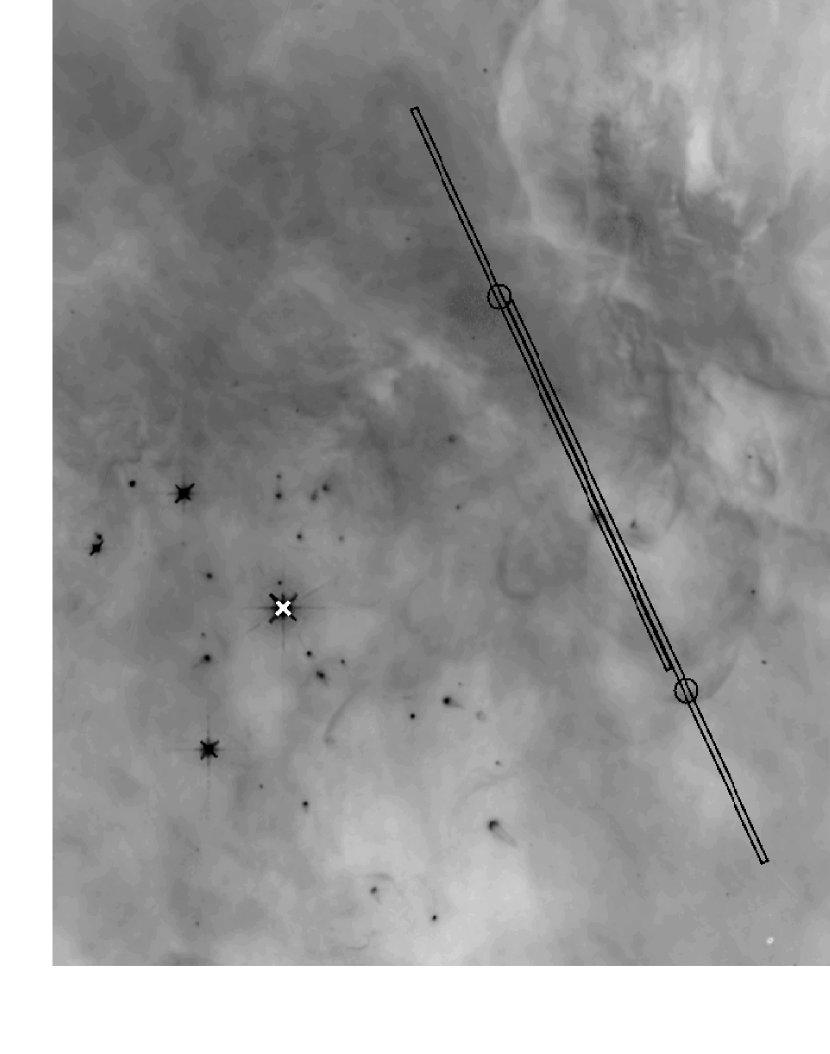
Figure 1: HST STIS Slit 1 ($52\arcsec\times 0.5\arcsec$, right) and Slit 2 (left) shown overlapping with HST FOS positions 1SW (right circle) and x2 (left circle) (Baldwin et al., 1996; Rubin et al., 1997), respectively. Slit positions are overlaid on F656N (H$\alpha$) WFPC2 image. $\theta^{1}$ Ori C is marked with a $\times$. N is up and E to the left.

HST FOS and STIS spectra were obtained with spectral coverage from the UV (1600Å) through to the visible (7400Å) for two lines of sight (roughly 1SW and x2, Baldwin et al., 1996; Rubin et al., 1997). The FOS aperture has a diameter $0\farcs 86$ and the STIS slit is $52\arcsec\times 0\farcs 5$ (refer to Fig. 1) of which only (the roughly central) $28\arcsec$ are recorded using the STIS UV detectors (FUV-MAMA, NUV-MAMA). The UV and optical spectra were adjusted to align spatially using a bright feature common to all spectra: proplyd 159-350 (O’Dell & Wen, 1994).

The placement of Slit 1 (see Fig. 1) was such that it was centered on a region of the nebula where there is an extinction gradient. Because of this, we divided the $52\arcsec\times 0\farcs 5$ slit into four $13\arcsec\times 0\farcs 5$ sections, labeled “a” through “d”. The different spatial coverage of the MAMA and CCD detectors means that the outer two sections (SLIT1a and SLIT1d) have reliable coverage only in the visible, but the central two sections (SLIT1b and SLIT1c) have coverage in the visible and the UV. The same sectioning was done for Slit 2 (x2, see Fig. 1). However, there was little change in the extinction across Slit 2 so the two central sections (SLIT2b and SLIT2c) should be similar.

The reduction of STIS spectra was performed as in Rubin et al. (2003) and the reduction of FOS spectra as in Rubin et al. (1998). Our HST STIS (SLIT1b, SLIT1c, SLIT2b, SLIT2c) and FOS (1SW) observations are presented in Table 1.

A wavelength-dependent extinction correction must still be applied to the entire spectrum (UV through visible/near-IR). To date, there has not been a robust way of reliably correcting such a large portion of the spectrum to allow for full (i.e., UV through visible) spectral analysis. However, with the broad spectral coverage of the HST data, we are able to develop and test a smooth consistent extinction correction curve. The development and validation of such an analytic extinction curve is discussed in § 3. To ensure that any extinction curve is well constrained, we must maximize the number of lines used in its determination. In § 4, we discuss the basis for the inclusion of He i (especially He i UV) lines.

3 Extinction corrections

Were it not for extinction, the Orion Nebula would appear much brighter. Typical optical depths reported are $\tau_{V}\sim 1$ . From the shape of the extinction curve (e.g., see curves in Kim et al., 1994), the optical depth in the Lyman continuum ($\tau_{912}$) would be several times this value. The relatively soft radiation from the primary ionization source (O star, $\theta^{1}$ Ori C) cannot photoionize an optical depth to dust of much more than $\tau_{912}\sim 1$ indicating that a large part of the optical extinction must come from neutral material in the foreground. Further evidence for and properties of this “veil” are summarized by Abel et al. (2004).

All observed emission-line surface brightnesses or fluxes, from the infrared to ultraviolet, are affected by this wavelength-dependent extinction and must be corrected before further analysis and interpretation. Extinction is characterized by its wavelength dependence (shape) and the amount at a given wavelength (amplitude).

Stellar extinction deduced from stars in the nebula provides a useful reconnaissance of the shape of the Orion Nebula extinction curve, providing a continuous curve with which to make predictions (by interpolation) for any given line observed. We have reconsidered the wavelength dependence of the infrared, optical and ultraviolet extinction, presenting our results as a convenient analytic expression describing this shape (“normalized extinction curve”) in § 3.1.1. The amplitude by which to scale the normalized extinction curve can be determined for a given line of sight from nebular lines whose ratios of line emissivities are known from atomic theory (e.g., H i Balmer series). An optimal implementation is discussed in § 3.1.2. In § 3.2, we compare our extinction curve with the nebular extinction curve of CP70. In § 3.3, we discuss our extensive validation of the use of our stellar-based extinction curve for interpolating corrections to the nebular emission in the optical, the ultraviolet and the near-infrared.

3.1 Parameterization of extinction

We have already stressed how one requires a shape ($s_{\lambda}$) and amplitude ($a$) to describe the extinction:

$$\tau_{\lambda}=a\,s_{\lambda}.$$ (1)

For different lines of sight, grain properties like size distribution and composition are manifested in $s_{\lambda}$, while $a$ scales with the column density of dust.

Let $F$ represent the observed flux of a patch of nebula (surface brightness times solid angle) or of a star, with subscript $o$ indicating the intrinsic flux – as it would have been had it not been affected by extinction $\tau$. (The dependence on wavelength $\lambda$ has been suppressed.) Thus $F/F_{o}=\exp(-\tau)$. For a uniformly bright nebular patch this is also the ratio of the specific intensities, $I/I_{o}$. Note that $I_{o}$ can be predicted by atomic theory, from the emissivity $j$ and (for most lines) the emission measure (Osterbrock, 1989). We adopt $I_{o}\propto j$ in the applications here, so that

$$F_{\lambda}={\rm constant}\times j_{\lambda}\;\exp(-a\,s_{\lambda}).$$ (2)

The logarithmic (base 10) extinction is $C=-\log(F/F_{o})=-\log(\exp(-\tau))=0.4343\tau$. The extinction in magnitudes is $A=-2.5\log(F/F_{o})=2.5C=1.086\tau$. Given the linear transformations between $A$, $C$, and $\tau$, a ratio like $A_{\lambda_{1}}/A_{\lambda_{2}}$ evaluated for two wavelengths is clearly interchangeable with the same ratio for $C$ or $\tau$.

In the literature there are various parameterizations of $A$, $C$, and $\tau$ that are worth distinguishing, since they imply different choices and normalizations of $s_{\lambda}$. Osterbrock (1989) uses $s_{\lambda}=0.5\tau_{\lambda}/(\tau_{\mathrm{H}\gamma}-\tau_{\mathrm{H}\alpha})$ and comments on the utility of the differential form $s_{\lambda}-s_{{\mathrm{H}}\beta}$. Note that he uses the notation $f_{\lambda}$ where we use $s_{\lambda}$.

For nebular extinction, one often writes the logarithmic extinction as $C_{\lambda}=C_{{\mathrm{H}}\beta}(1+f_{\lambda})$, with $f_{{\mathrm{H}}\beta}=0$ (e.g., Peimbert & Torres-Peimbert, 1977). Then if we adopt $s_{\lambda}=(1+f_{\lambda})\equiv\tau_{\lambda}/\tau_{{\mathrm{H}}\beta}$ we have $a=C_{{\mathrm{H}}\beta}/0.4343=\tau_{{\mathrm{H}}\beta}$.

For stellar extinction one often adopts the normalization $s_{\lambda}=A_{\lambda}/A_{V}\equiv\tau_{\lambda}/\tau_{V}$ (e.g., CCM89) in which case $a=A_{V}/1.086=\tau_{V}$. In order to compare these differently normalized nebular and stellar extinctions, one can easily show that

$$1+f_{\lambda}=\frac{A_{\lambda}/A_{V}}{A_{{\mathrm{H}}\beta}/A_{V}}.$$ (3)

Differential extinction between two wavelengths can of course be defined in any system. For example, color excesses are differences in magnitudes, like $E_{B-V}=A_{B}-A_{V}$. These can lead to differential extinction curves with new normalizations, like $E_{\lambda-V}/E_{B-V}=(A_{\lambda}-A_{V})/E_{B-V}=R_{V}(A_{\lambda}/A_{V}-1)$, accompanied by the introduction of new parameters, like the ratio of total to selective extinction, $R_{V}=A_{V}/E_{B-V}$.

3.1.1 Determining the shape, $s_{\lambda}$: Stellar extinction

CCM89 defined the shape of optical stellar extinction analytically using a single parameter, $R_{V}$, to describe differences between lines of sight. The shape has been adopted in many investigations of the Orion Nebula (Baldwin et al. 1991; Osterbrock et al. 1992, hereafter OTV92; Greve et al. 1994), with $R_{V}=5.5$.

Optical Good optical spectrophotometry of the Orion stars ($\theta^{1}$ and $\theta^{2}$) is presented by Cardelli & Clayton (1988) (hereafter CC88) as $E_{\lambda-V}/E_{B-V}$. Using measurements from their graphs, we show that the optical data (and more scanty infrared data) are fit well by the CCM89 formula (dash-dotted line in our Fig. 2). The CC88 data (asterisks in Fig. 2) continue to about 3 µm^-1 and show that there is a knee in the CCM89 curve at about 2.7 µm^-1 ($\lambda$3700) that is perhaps a bit too high and sharp. Therefore, an analytic modification has been made to the CCM89 formula (solid line) to round off the knee smoothly between 2.3 and 3.3 µm^-1, fitting the CC88 data quite well.

Ultraviolet The ultraviolet data come from IUE measurements by Bohlin & Savage (1981) (hereafter BS81) for the same Orion stars (see Fig. 2). The BS81 points (x) do not join on smoothly to the CC88 optical data. CC88 reanalyzed the ultraviolet data, showing how it could reasonably be joined smoothly to their new accurate optical spectrophotometry (asterisks). The main effect on the BS81 data (x) is to move it up slightly ($\sim 0.25$ mag shift), concomitantly increasing the expected ultraviolet extinction (see Fig. 2).

Note that in the ultraviolet, the analytic CCM89 formula does not fit either the CC88 or BS81 observations: the predicted bump is too strong. However, it is possible to adjust a few constants in the CCM89 formula to obtain a modified CCM89 curve (solid line) that runs smoothly through the CC88 data.

To gauge the importance of these modifications for the determination of extinction-corrected fluxes, consider the situation for the N ii] $\lambda\lambda$2140-43 pair near the peak of the extinction curve. The unmodified CCM89 curve exceeds ours by $\delta E_{\lambda-V}/E_{B-V}=0.85$. For a typical value $E_{B-V}=0.3$ the difference would be $\delta\tau=0.23$; thus the N ii] line would be 26% (0.1 dex) stronger if corrected according to the unmodified CCM89 curve.

Near infrared Near 1 µm the CCM89 $A_{\lambda}/A_{V}$ curve becomes a power law in $\lambda^{-1}$ of index 1.6. Most stellar curves exhibit this “common power law” region of the extinction curve, independent of $R_{V}$ (Martin & Whittet, 1990). The latter analysis suggests an index of 1.85, which we adopt in our extinction curve. This modification will not have an impact here, as the observations analyzed do not extend much beyond 1 µm.

We have included a table of $f_{\lambda}$ values for a number of observed emission line wavelengths (see Table 2), calculated directly from our modified set of CCM89 equations (with $R_{V}=5.5$). For other wavelengths, refer to CCM89 and our analytic modifications discussed above.

3.1.2 Setting the amplitude, $a$: Optimal fitting of emission lines

Measurements of emission lines in nebulae are often used to gauge the extinction (e.g., CP70; OTV92; Greve et al. 1994; Esteban et al. 1998, hereafter EPTE98; Esteban et al. 2004, hereafter EPG04). If the shape $s_{\lambda}$ of the extinction curve is known, then the amplitude $a$ in equation 2 can be determined with even a single line pair from the same ion, assuming the relevant emissivities $j_{\lambda}$ are known. The Balmer and Paschen lines are popular as their emissivities are well described by H i recombination theory and can be computed readily for various electron temperatures ($T_{e}$) and densities ($N_{e}$). See Storey & Hummer (1995) for detailed access to the results of their computations using an interactive data server. For the illustrations below we adopt case B emissivities with $T_{e}=8000$ K, $N_{e}=2500$ cm^-3 for FOS-1SW and STIS-SLIT1c (as determined from nebular models presented in § 4.4), $T_{e}=9000$ K, $N_{e}=5000$ cm^-3 for the remainder of the STIS slits, and $T_{e}=8300$ K, $N_{e}=8900$ cm^-3 for the EPG04 observations (as determined from their temperature and density diagnostic ratios). Lines from other ions can be useful too (e.g., He i, [O ii], [S ii]), as further illustrated in § 4 (He i) and § 3.3 ([O ii], [S ii], He i).

Method Sometimes the amplitude is taken from only one line ratio, like H$\alpha$/H$\beta$, but often other lines are available too. Past methodology has been to form various line ratios, compute the amplitude (e.g., the equivalent $A_{V}$) from each independently (sometimes with discrepant results), and then compute some average. A new approach adopted here is to fit the observed line fluxes directly to equation 2, not forming line ratios at all. The fit is carried out straightforwardly by non-linear least squares, with two unknowns: $a$ and a constant multiplier (which is proportional to the ionic abundance through the emission measure.) In addition, from the goodness of fit of the data to the model, we obtain the $1\sigma$ confidence intervals on the parameters. This approach has some advantages: avoiding the inevitable bias from errors in the chosen normalizing line(s), using a standard treatment of the measurement errors to weight the fit and hence avoiding the ambiguity associated with deciding what average amplitude to compute.

If later one wants to tabulate extinction-corrected line ratios relative to, say, H$\beta$ (or He i 4471 if He i lines are used in the extinction fitting), then the extinction model gives the best estimate of the corrected flux for this normalization, optimally consistent with all other lines in the series. When the He i recombination lines are fit simultaneously, then the optimal He⁺/H⁺ ratio is obtained, along with its formal error, without reference to particular He i to H i dereddened line ratios.

3.2 Comparison between stellar and nebular extinction curves

The CP70 nebular extinction curve is an alternative commonly used in the calculation of the extinction correction (EPTE98; EPG04). This curve was determined from optical and radio observations of four lines-of-sight in the Orion Nebula. The radio (1.95 cm) observations are used to determine the absolute extinction, $A_{{\mathrm{H}}\beta}$, and the piecewise normalized extinction curve, $1+f_{\lambda}$, is obtained for various lines:

$$f_{\lambda}=\frac{E_{\lambda-{\mathrm{H}}\beta}}{A_{{\mathrm{H}}\beta}}.$$ (4)

Calculations of $C_{{\mathrm{H}}\beta}$ offer a simple means by which to compare our modified CCM89 curve with that of CP70. Performing a least-squares analysis on EPG04 data using the CP70 curve (and interpolations thereof), we get $C_{{\mathrm{H}}\beta}=0.65\pm 0.03$, as compared to $C_{{\mathrm{H}}\beta}=0.85\pm 0.04$ when we use our extinction curve. EPG04 had $C_{{\mathrm{H}}\beta}=0.76\pm 0.08$ when using this same series (up to H15, $\lambda$3712) of H i lines. However, this comparison of $C_{{\mathrm{H}}\beta}$ is not enough. The shape of the CP70 curve is investigated more thoroughly in the following sections.

3.2.1 Infrared discrepancy

The zero-point is calculated by CP70 using radio data at (more or less) the same spatial position as the optical data. The rest of CP70’s $f_{\lambda}$ is determined directly from specific Balmer or Paschen lines (as tabulated in Peimbert & Torres-Peimbert, 1977), so that most of the curve plotted in Figure 3 is interpolated (by CP70; Peimbert & Torres-Peimbert, 1977; Walter, 1993).

Near 1 µm^-1, the CP70 curve is dramatically below our extinction curve (see Fig. 3). This is getting into the “common power law” region of the extinction curve mentioned in § 3.1.1. Nowhere is there evidence for the strong curvature implied in the CP70 extinction curve in the region from 1 µm^-1 to zero wavenumber. The IR discrepancy might simply be the result of an inappropriate interpolation of the CP70 extinction curve. Looking at Figure 1 of CP70, it appears as if other interpolations to the $V$ band are possible. If the interpolated $f_{V}$ were a bit more negative ($-0.12$ or $-0.13$ instead of $-0.094$ would seem reasonable) and the CP70 curve (shown in our Fig. 3) was refit (and rescaled, see below), it would be noticeably closer to the stellar one from the optical through the near infrared.

The change in the interpolated $f_{V}$ would affect $R_{V}$ as derived from

$$R_{V}=\frac{1+f_{V}}{f_{B}-f_{V}},$$ (5)

resulting in $R_{V}=4.5$ ($f_{V}=-0.12$) or 4.2 ($f_{V}=-0.13$) compared to the CCM89 and CP70 value of $R_{V}=5.5$. However, the $f_{\lambda}$ depend on comparing radio and optical data (see equation 4). This radio/optical comparison is almost certainly affected by a 10-20% reflection effect in the optical (e.g., Henney, 1998). Because of reflection, the lines like H$\beta$ are measured to be too bright relative to the radio, resulting in a low estimate of the absolute extinction, $A_{{\mathrm{H}}\beta}$. In the optical where the differential extinction $E_{\lambda-{\mathrm{H}}\beta}$ is not affected much by reflection, $f_{\lambda}=E_{\lambda-{\mathrm{H}}\beta}/A_{{\mathrm{H}}\beta}$ will be too high. A typical logarithmic extinction $C_{{\mathrm{H}}\beta}$ ($C_{{\mathrm{H}}\beta}=0.4A_{{\mathrm{H}}\beta}$) is 0.5, so that with $f_{V}=-0.12$, the logarithmic extinction at $V$ is $0.5\times(1-0.12)=0.44$ or $A_{V}\sim 1$. A 20% reflection effect at $V$ would cancel out real extinction at the level $\Delta~{}A_{V}=0.2$, lowering what should be 1 to 0.8 (apparent). Then $0.8\times 5.5$ predicts $R_{V}$(apparent)$=4.4$. Both the sign and order of magnitude of the reflection correction appear to be right. Note that there are other possibilities of systematic error as the radio/optical comparison also depends on the adopted temperature, matching the spots observed, etc.

To remedy this artificial alteration of $R_{V}$, we introduce a correction to $A_{{\mathrm{H}}\beta}$ – effectively a rescaling of $f_{\lambda}$ – to maintain $R_{V}=5.5$. With $f_{V}=-0.12$ in our new interpolation of the CP data, one needs to divide all $f_{\lambda}$ by a factor 1.198 to ensure that $R_{V}=5.5$. This rescaled CP70 absolute extinction curve is presented in Figure 3.

The shape of our rescaled CP70 curve in the visible is similar to that of our modified CCM89 curve and so regardless of which of these is used, one should be able to get good differential fits to a series of optical lines. The differential extinction between H$\alpha$ (1.52 µm^-1) and H$\delta$ (2.44 µm^-1) is the same in both curves, and one obtains more or less the same $C_{{\mathrm{H}}\beta}$ when fit to the Balmer lines, independent of the choice of curve (see § 3.3.1).

3.2.2 Ultraviolet

Walter (1993) extended the CP70 curve to the ultraviolet by attaching on the BS81 data assuming $R_{V}=5.5$. This extended extinction curve was also described by Rubin et al. (1993). We have derived $f_{\lambda}$ values from the original BS81 $E_{\lambda-V}/E_{B-V}$ form (as in Rubin et al., 1993) for both the CP70 and rescaled CP70 curves, generating a shape of the ultraviolet extinction for each, as seen in Figure 3. This extension lies below the CC88 revision of the BS81 data in the ultraviolet and does not join smoothly to the optical portion of the CP70 curve. One of the reasons is that the CP70 curve has been extrapolated to $\lambda$3500 (see their Table 2), incorrectly high, beyond the highest Balmer transitions that were observed (H9, $\lambda$3835). When combined with the ultraviolet data (BS81 version) this really sticks out as a kink in the curve at $\lambda$3500; a smooth join, like all (stellar) extinction curves observed, is not possible. The reddening correction of a line like [O ii] $\lambda$3727 would be in doubt. Our modified CCM89 curve seems a more reliable alternative in this “extrapolated” region.

3.3 The stellar extinction curve: validation

It is important to address whether the shape of extinction derived from stars is appropriate for diffuse nebular emission, where the presence of scattered light might be an issue. We have therefore carried out extensive tests of this technique using consistent sets of nebular measurements of hydrogen lines in Orion, both from the literature (CP70; Peimbert & Torres-Peimbert 1977; OTV92; EPTE98; EPG04) and from our HST and ground-based (Baldwin et al. 2000, hereafter BVV00; Blagrave et al., 2006a, b) observations.

Here we exploit our HST FOS and STIS (SLIT1c) observations for the line of sight 1SW (see Table 1) as, with the addition of several UV lines, they offer an extensive spectral range for the validation. As will be discussed here, and again in § 4.6 (Figures 9 and 10), the data are well fit using our extinction curve.

3.3.1 Optical

In addition to our own STIS and FOS observations we have used others’ observations to examine the fit of the stellar-derived extinction curve in the optical. Using the extensive observations of EPG04, we have determined the best-fit extinction curve (see § 3.1.1) using the unblended H i Balmer lines (up to H17, $\lambda$3697) and Paschen lines (up to P18, $\lambda$8438), resulting in $C_{{\mathrm{H}}\beta}=0.82\pm 0.04$. The resulting curve and residuals from this fit are shown in Figure 4. Over the spectral range that can be accessed by these lines, the fit is good, demonstrating that our extinction curve provides a good empirically-derived interpolation formula for differential extinction.

The EPG04 data were also fit using the scaled form of CP70 developed in § 3.2 and the same H i lines as above. The resulting curve and residuals are included in the bottom panel of Figure 4. We find $C_{{\mathrm{H}}\beta}=0.76\pm 0.04$, in agreement with $C_{{\mathrm{H}}\beta}=0.76\pm 0.08$ found by EPG04. As shown in the top and bottom panels of Figure 4 and discussed in § 3.2, the differential extinction is well represented by both our scaled CP70 and modified CCM89 curves.

We have also carried out fits of the various data sets using our curve and $R_{V}=3.1$, appropriate to the diffuse interstellar medium (Savage & Mathis, 1979). By comparison to the Orion curve (with $R_{V}=5.5$) this curve is steeper throughout the optical, producing relatively less (more) extinction compared to H$\beta$ in the near-infrared (blue). This produces a markedly inferior fit.

3.3.2 Ultraviolet

Validation using nebular observations is especially important for the ultraviolet portion of the extinction model. The STIS and FOS spectra include the common upper level pair [O ii] $\lambda\lambda 2471,7325$ which can be used in this validation.

The [O ii] $\lambda$2471 line is actually a blend of transitions from ${}^{2}P_{1/2}$ and ${}^{2}P_{3/2}$ to ${}^{4}S_{3/2}$ (Osterbrock, 1989). Transitions from these upper levels also lead to the formation of a pair of blended near-infrared lines. Each upper level contributes a line to a blend at $\lambda$7321 (transitions to ${}^{2}D_{5/2}$) and another line to a blend at $\lambda$7332 (transitions to ${}^{2}D_{3/2}$); the combined near-infrared line will be denoted $\lambda$7325. Thus the $I_{2471}/I_{7325}$ line ratio is not quite the ideal case with a single common upper level in which the emissivities of the line pair are simply proportional to the radiative transition probabilities divided by the respective wavelengths. Instead, this line ratio depends on the collisional excitation of ${}^{2}P_{1/2}$ relative to ${}^{2}P_{3/2}$. However, calculations with a five-level atomic model show that the line ratio is not very sensitive to $T_{e}$ and $N_{e}$ over the range expected in the Orion Nebula. We adopt 0.75 using modern collision strengths (Pradhan et al., 2006) and older transition probabilities (Zeippen, 1982). We compare these results with a second ratio, 0.81 derived using the modern set of transition probabilities recommended by Wiese et al. (1996). These are both calculated for $T_{e}=8000$ K and $N_{e}=2500$ cm^-3 (see § 4.4).

In Table 3, the predicted $I_{2471}/I_{7325}$ ratios are compared to our observed ratio corrected using our extinction curve and H i lines. Use of the modern transition probabilities results in a 15-20% over-prediction, whereas the older transition probabilities result in a slightly lower 10-15% over-prediction. These modern transition probabilities have been found to yield anomalous density and temperatures from [O ii] lines (see Wang et al., 2004; Blagrave et al., 2006a, EPG04) and thus it is not unexpected that the older transition probabilities yield a slightly more consistent result.

As a check on the theoretical predictions, we have also examined the [O ii] $I_{7321}/I_{7332}$ line ratio which is slightly more sensitive to the relative upper level populations, but not sensitive to the applied reddening correction. The prediction is 1.25 using Zeippen (1982) transition probabilities and 1.23 using Wiese et al. (1996) transition probabilities. Our ratios are 1.21-1.24 for the STIS observations. Other observations in Orion by OTV92 give 1.134, while BVV00 find 1.25 and EPG04 find 1.30. Our ability to accurately predict (within 15%) both the $I_{7321}/I_{7332}$ line ratio and the common-upper-level line ratio $I_{2471}/I_{7325}$ supports the validity of our analytic extinction curve in the UV. However, it would be beneficial to have further constraints in the UV. This is addressed in § 4.

3.3.3 Near infrared

Similarly, the [S ii] common upper-level line pair $I_{10300}/I_{4072}$ can be used to confirm the validity of the extinction curve in the infrared. Our data do not extend into the infrared, but those of EPG04 do. The three observed lines at $\lambda 10300$ and two at $\lambda 4072$ have been corrected for extinction using our best-fit extinction curve (see § 3.3.1). Since this is a ratio being used for validation and is not in the fit, the visible line (which tends to have the lower error) has been set to $I_{corrected}/I_{predicted}=1$ in Figure 4. The agreement is good.

As pointed out in Porter et al. (2006), EPG04 have also observed a series of He i common upper-level line pairs. These line pairs have been overplotted on Figure 4 too. The IR pair members have $I_{corrected}/I_{predicted}=1.2\pm 0.5$. While there are large differences between the observed and predicted line strengths, there is no significant systematic bias, indicating that our extinction curve is also valid between the near-IR and near-UV.

4 Anomalous He i decrements

Based on predictions from recombination theory we have used the H i Balmer and Paschen series to calibrate the reddening curve. The same should be possible using recombination theory (Smits, 1996; Benjamin et al., 1999; Porter et al., 2005) and observations of the He i lines (see energy-level diagrams in Fig. 5).

4.1 Extinction-corrected data

Table 4 presents our He i data from FOS-1SW and (the section of our STIS spectrum that covers 1SW) STIS-SLIT1c observations as well as complementary data from comprehensive ground-based studies by OTV92, EPTE98, BVV00, and EPG04.

Each of the He i lines has been corrected for reddening using our best-fit curve as normalized using the observed H i Balmer (and Paschen, where available) series lines, and each line’s case B prediction. Case B predictions depend on $T_{e}$ and $N_{e}$ (Storey & Hummer, 1995) and so are unique to each observation set: $T_{e}=9000$ K, $N_{e}=4000$ cm^-3 (OTV92); $T_{e}=9500$ K, $N_{e}=5700$ cm^-3 (EPTE98, position 2); $T_{e}=9000$ K, $N_{e}=5000$ cm^-3 (BVV00); $T_{e}=8300$ K, $N_{e}=8900$ cm^-3 (EPG04); $T_{e}=8000$ K, $N_{e}=2500$ cm^-3 (FOS-1SW, STIS-SLIT1c).

As is common, the line strengths are given relative to the singlet line $\lambda$4471.

The quoted uncertainties for OTV92 and EPTE98 are estimated from their description of the quality of the data. Those of EPG04 are directly from the per cent errors in their Table 2. BVV00 and FOS-1SW uncertainties were determined using the signal to noise ratio, $S/N$, as found from fitting each emission line to a five-parameter (area, central wavelength, FWHM, continuum baseline and continuum slope) single Gaussian model. This $S/N$ is combined with the integrated line flux to produce the uncertainty. The STIS data is similarly fit with a model which takes into account the $0\farcs 5$ STIS slit width (see Appendix A in Rubin et al., 2003). Again, the resultant $S/N$ from this fit is combined with the integrated flux to determine the uncertainty.

4.2 Case B

He i case B predictions for FOS-1SW and STIS-SLIT1c $T_{e}$ and $N_{e}$ ($n\leq 5$, Porter et al. 2005; $n>5$, Smits 1996) are shown in column (3) of Table 4 and are quite representative for the range of nebular densities and temperatures we consider.

Most of the reddening-corrected singlet and triplet lines (cols. (6)-(11)) are well-approximated by case B recombination alone (col. (3)).

In comparing their case B results with the OTV92 observations, Benjamin et al. (1999) noted (their Figs. 2a and 2b) that the lines (singlets and triplets) shortward of $\lambda$3820 were consistently brighter than predicted, increasingly with decreasing wavelength, except $\lambda$3188 which appeared to be accurately predicted. They suggested that this upward trend shortward of $\lambda$3820 could be due to unaccounted for radiative transfer effects, though this seems very unlikely given the lines involved. Inclusion of radiative transfer (see discussion below) would cause the plotted $\lambda$3188 ratios to increase – possibly enough to agree with the apparent upward trend shortward of $\lambda$3820 – while not affecting the other lines shortward of $\lambda$3820. If alternatively this upward trend arose from inadequate/unmodeled extinction corrections, there would have to be a very sudden (relative) decrease in the extinction in order for the extinction-corrected lines not to appear so bright. It is informative to note that the discrepancy in this instance cannot be explained by the inaccurate extrapolation of CP70 as discussed in § 3.2.2 (since CP70 is not used in the extinction correction). It seems most probable that there is a systematic problem with the absolute calibration used and/or significant measurement errors due to strong atmospheric extinction varying rapidly with wavelength for $\lambda<3500$ Å (OTV92). See also § 4.5, Figure 8.

In their discussion of nebular model predictions of the He i lines compared to the EPG04 observations, Porter et al. (2006) have noted that He i lines of the $2~{}^{1}S~{}-~{}n~{}^{1}P$ series in the same wavelength range ($\lambda\lambda 3448,3355,3297$) are also brighter than the expected case B predictions. Analyzing the line ratios between successive members of this series (their Figs. 1 and 5) they conclude that there are problems with these observational results, possibly with the extinction (over-)correction. The same observations, corrected according to our best-fit extinction curve, are presented in Table 4, where it can be seen that the observations and case B (or our full models) are in agreement within the errors.

As seen in Table 4, use of our extinction curve brings $\lambda$7281 into agreement with the case B predictions (as suggested by Porter et al., 2006). Many of the other near-IR lines observed by EPG04 are still scattered about the best-fit expectation (Table 4 and graphically in § 3.3.3, Figure 4). These infrared lines are difficult to observe because of atmospheric effects (OTV92) and the errors might be underestimated (Porter et al., 2006), but the important thing to note is that there does not appear to be any systematic discrepancy – except as noted below for the infrared lines of the triplet series $3~{}^{3}S~{}-~{}n~{}^{3}P$.

4.3 Anomalous decrements

Despite the validity of case B for the prediction of most lines, there remains a systematic mismatch between observed and predicted ratios for a number of the He i lines from the series $2~{}^{3}S~{}-~{}n~{}^{3}P$, $2~{}^{3}P~{}-~{}n~{}^{3}S$, $3~{}^{3}S~{}-~{}n~{}^{3}P$, and $2~{}^{1}S~{}-~{}n~{}^{1}P$.

For the triplet lines, the underlying reason is the metastability of the $2~{}^{3}S$ term which can only be depopulated via photoionization, through collisional transitions to $2~{}^{1}S$ and $2~{}^{1}P$, or through the (strongly forbidden) radiative transition $1~{}^{1}S~{}-~{}2~{}^{3}S$ (Osterbrock, 1989). The visible/near-UV lines of the $2~{}^{3}S~{}-~{}n~{}^{3}P$ series (including $\lambda\lambda$3889, 3188, 2945, 2829, etc.) are affected by self-absorption from the metastable $2~{}^{3}S$ term to the corresponding $n~{}^{3}P$ term. This results in case B recombination theory over-predicting these lines (see Table 4). Note that although $\lambda 3889$ is blended with a Balmer line, it is still possible to predict the observed intensity of the He i component and use it as a valuable diagnostic. For the entries in Table 4 we used case B H i predictions and the He⁺/H⁺ derived from the other lines to deblend $\lambda$3889; this also enables a “case B” prediction for the blend (see col. (3) in Table 4). The space-based observations that we report here are particularly valuable for verifying the expected diminution of this self-absorption effect in higher members of the series. This appears to be the case as discussed in the modeling below.

For self-consistency, there must also be a detectable resonance fluorescence enhancement of the $2~{}^{3}P~{}-~{}n~{}^{3}S$ series as some of the electrons promoted by self-absorption to $n~{}^{3}P$ radiatively cascade back down to $2~{}^{3}S$ via alternate routes. Indeed, this is quite evident in the $2~{}^{3}P~{}-~{}n~{}^{3}S$ series, primarily in $\lambda$7065 ($n=3$), but detectable in $\lambda$4713 ($n=4$) and $\lambda$4121 ($n=5$) too (see Table 4). Similarly, we expect to see an enhancement of other triplet series including the near-IR series, $3~{}^{3}S~{}-~{}n~{}^{3}P$. The data in Table 4 show this enhancement. We will return to analysis of these series in § 4.5.

The singlet lines of the series $2~{}^{1}S~{}-~{}n^{1}P$, $\lambda$5016 ($n=3$) (and to a much lesser extent $\lambda$3965, $n=4$) are also observed to be consistently less than the case B prediction. As discussed in Porter et al. (2006), this is most probably a result of UV lines ($\lambda$537, $1~{}^{1}S~{}-~{}3~{}^{1}P$ and $\lambda 522$, $1~{}^{1}S~{}-~{}4~{}^{1}P$) escaping the nebula, resulting in case B being shifted slightly toward case A (as defined in Baker & Menzel, 1938).

4.4 Photoionization models

The CLOUDY photoionization code (Ferland et al., 1998) accounts for many radiative transfer effects, including those relating to the metastable $2~{}^{3}S$ term. It is also possible to run CLOUDY models that exclude all line transfer in order to investigate its importance. With this in mind, a series of CLOUDY photoionization models was developed.

Self-absorption effects depend on the line width because this affects the opacity. The He i lines (among others) observed in the ground-based echelle spectra (BVV00; Blagrave et al., 2006a, b) have line widths (FWHM) in excess of the Doppler/thermal and instrumental widths. When the Doppler/thermal and instrumental widths are subtracted (in quadrature) from the measured FWHM there remains an unaccounted for contribution to the broadening which has been labeled as “turbulence”. In the case of the He i singlet lines (which do not have any fine-structure levels and therefore will not have any further FWHM contribution from a line blend) in the 1SW ground-based echelle spectra (Blagrave et al., 2006b), we find FWHM${}_{turb}=15.5\pm 2.4$ km s^-1. This is quite consistent with the “turbulence” contribution quoted in O’Dell et al. (2003) for the He i $\lambda$5876 triplet line: $18.4\pm 2.9$ km s^-1. This latter line and other triplet lines have another broadening contribution brought on by transitions in the fine structure ($J$ levels) and therefore are slightly less reliable in the determination of the additional “turbulence” contribution. As was mentioned in O’Dell et al. (2003) and is also found here, the magnitude of the “turbulence” contribution to the line width appears to decrease as one probes along the line of sight from cooler (associated with H i and He i) to hotter (associated with [O iii], [O ii], [S ii], etc.) regions of the nebula. As the He i recombination lines preferentially probe the cooler region of the nebula, the “turbulence” that these lines reveal is an upper limit for the nebular model.

This turbulent contribution to the line width will affect the magnitude of the radiative transfer effect on the $2~{}^{3}S-n~{}^{3}P$ series of lines (and the related lines, like $\lambda$7065), as it broadens the lines and lowers the effective optical depth and line trapping. The effects from radiative transfer should diminish as the turbulence is increased. To investigate the effects of this change in turbulence on line predictions, we developed a series of constant density ($10^{4}$ cm^-3) and constant temperature ($10^{4}$ K) CLOUDY models each with a different turbulence parameter, $v_{turb}=\mathrm{FWHM}_{turb}/\sqrt{4\ln 2}$ (as defined in CLOUDY), and excluding “induced processes” (as defined in CLOUDY, these include continuum fluorescent excitation and induced recombination). Then each of these constant-turbulence models was varied in thickness, in order to develop plots of line ratios as a function of $\tau_{0}$($\lambda 3889$) – the optical depth at the center of He i $\lambda$3889 for zero turbulence velocity (see Fig. 6). For the normalizing line we use $\lambda$4471 which is not significantly affected by radiative transfer. Our Figure 6 can be compared with Figure 4.5 of Osterbrock (1989), which shows similar variation, but in the latter case as a result of changes in the nebular expansion velocity. At $\tau_{0}=0$ all models reduce, as is expected, to their case B values.

Figure 7 plots the line strengths, $I_{\lambda}/I_{\lambda 4471}$, as a function of each model’s “turbulence” parameter for fixed $\tau_{0}$($\lambda 3889$)$\sim 27$ which is appropriate to the column density of our full nebular model below. In this case to enable the best comparison between the CLOUDY model predictions and our observations, the “induced processes” are included (regardless, in our full model the relative importance of the induced processes is much diminished because the nebula becomes optically thick to the continuum radiation responsible for these excitations). From the overplotted observed $I_{\lambda 7065}/I_{\lambda 4471}$ in Figure 7, we would predict $v_{turb}=20-30$ km s^-1, whereas from $\lambda 3889$ (deblended), $\lambda 3188$ and $\lambda 2945$, $v_{turb}=10-12$ km s^-1. This latter prediction is consistent with the “turbulence” contribution (FWHM${}_{turb}\sim 16$ km s^-1; i.e., $v_{turb}\sim 10$ km s^-1) which was determined from the observed He i lines’ FWHM above. The value $v_{turb}=12$ km s^-1 will be adopted in the CLOUDY models discussed hereafter. Models with this value of the turbulence should be able to roughly explain the observations of the hitherto anomalous He i lines. As expected, the results of the full nebular models to be discussed (Table 4) are slightly different than the results for constant $N_{e}$ and $T_{e}$ in Figure 7, in particular giving even better agreement for $\lambda$7065.

Our full nebular models are similar to the Orion Nebula model discussed in Baldwin et al. (1991) – i.e., a closed geometry and constant pressure. Two such models (see Tables 5 and 6) were created, as was done in Blagrave et al. (2006a): one with a Mihalas stellar atmosphere model (Mihalas, 1972) and H ii region abundances as defined in CLOUDY (Baldwin et al., 1991; Rubin et al., 1991, OTV92) (model M); and one with a Kurucz stellar atmosphere model (Kurucz, 1979) and EPG04 Orion Nebula abundances (model K). The Mihalas (non-LTE) stellar atmosphere has been shown to best represent the incident continuum radiation (BVV00), but to test the robustness of our results we also include the Kurucz (LTE, line-blanketed) stellar atmosphere in our second model. Each of these models has $v_{turb}=12$ km s^-1. The other parameters (density, radius, etc.) were varied so as to best reproduce the SLIT1c H$\beta$ surface brightness and the temperature- and density-sensitive lines, as summarized in Table 7 for both models.

The models’ predictions of the He i lines given in columns (4) and (5) in Table 4 include the deviation from case B introduced by the metastable $2~{}^{3}S$ term. The effect of this metastability is reflected in the models’ (non-zero) line optical depth, $\tau$($\lambda 3889$)=13. Note that He i $\lambda$3889 ($n=3$) appears as a blend with H i $\lambda$3889 and He i $\lambda$2829 ($n=6$) appears as a blend with [Fe iv] $\lambda$2829. Neither of these blends is included in our quantitative analysis, but the predicted value for each is shown in a separate row in Table 4.

Models M and K were modified to exclude radiative transfer in order to further investigate the validity of the CLOUDY models. This exclusion has the expected effect on the lines: returning the triplet line predictions to roughly their case B values and those singlets connected radiatively to the ground state are reduced to their case A values.

4.5 Comparison with observations

We have modeled the extinction correction for OTV92, EPTE98, BVV00, EPG04 and our FOS-1SW and STIS-SLIT1c observations using our extinction curve and the H i Balmer (and Paschen, where available) lines and a subset of He i lines, excluding lines from the triplet series $2~{}^{3}S~{}-~{}n~{}^{3}P$ ($\lambda\lambda$3889, 3188, 2945, 2829), $2~{}^{3}P~{}-~{}n~{}^{3}S$ ($\lambda\lambda$7065, 4713, 4121) and $3~{}^{3}S~{}-~{}n~{}^{3}P$ (all lines) and the singlet line, $\lambda$5016. Our $C_{\mathrm{H}\beta}$ from the fit of H i and the subset of He i lines is consistent with that found using H i lines alone (see end of Table 4), suggesting that both H i and this subset of He i lines are reliable determinants of the extinction correction.

For comparison with these extinction-corrected observations, $I_{corrected}$, we adopt separately predictions, $I_{predicted}$, from case B and CLOUDY model M. Values of log($I_{corrected}/I_{predicted}$) are plotted in Figure 8 for all observed members of four series for both case B and model M predictions. Many data sets are shown, but EPTE98 is excluded simply to avoid visual clutter. For the $2~{}^{3}P~{}-~{}n~{}^{3}D$ series, which includes $\lambda$4471 ($n=4$), case B and model M are in close agreement. This triplet series is not significantly affected by radiative transfer effects and the theory and observations are in close agreement. The other triplet series are clearly affected, by self-absorption ($2~{}^{3}S~{}-~{}n~{}^{3}P$) or by resonance fluorescence enhancement ($2~{}^{3}P~{}-~{}n~{}^{3}S$, $3~{}^{3}S~{}-~{}n~{}^{3}P$). Case B is a poor approximation, but the agreement between theory and observations improves dramatically as we switch from case B to model M. ($\chi^{2}$ is reduced by a factor of roughly 10.)

Two features deserve further discussion. The OTV92 data shortward of 3700 Å (including $\lambda$3188) most likely suffer from systematic errors (§ 4.2). This can be seen graphically in the $2~{}^{3}P~{}-~{}n~{}^{3}D$ series of Figure 8 when comparing OTV92 (circles, no uncertainty bars) and others’ datasets; the OTV92 data points (with one exception, $\lambda$3479) all lie significantly apart from the other data. Second, $\lambda$9464 measured by EPG04 appears to be too faint. This line has a number of neighboring near-IR H i Paschen lines and He i lines which appear to be well-fit by our extinction correction. There would have to be a large sudden increase in the amount of extinction for the extinction correction to be able to account for this anomaly. This suggests that $\lambda$9464 may have a larger than reported measurement uncertainty (see also § 4.2 and Porter et al., 2006).

4.6 Extinction corrections revisited

The STIS and FOS data are corrected for extinction using our extinction curve, the unblended H i lines, the subset of He i lines and the common-upper-level pair of [O ii] lines (refer to § 4.5 and § 3.3.2). These are presented in Table 8 relative to the H$\beta$ predicted from the fit, along with the derived $C_{\mathrm{H}\beta}$.

In Figure 9, we show the extinction-corrected FOS-1SW line intensities compared to the case B theory (the residuals of the fit) as well as the extinction correction applied (here expressed differentially with respect to $C_{\mathrm{H}\beta}$). The He i lines $\lambda\lambda$7065, 3188, and 2945 are excluded from the fit, but their values relative to case B and model M predictions are overplotted. Model M provides a better prediction for the lines affected by radiative transfer.

The analysis for the SLIT1c data is shown in a similar way in Figure 10. The He i lines $\lambda\lambda$7065, 5016 and 2945 (and H i line $\lambda$3704, because of large uncertainty) are excluded from the fit, but their values relative to case B and model M are overplotted. Again, model M provides a better prediction for the lines affected by radiative transfer.

In fitting the UV extinction curve, we conclude that $\lambda$3889 (a blend in any case), $\lambda$3188, $\lambda$2945, and $\lambda$2829 (also a blend) should be excluded – pending correction for radiative transfer effects – but that lines associated with higher $n$ (i.e., $n>6$) can be included to ensure a more robust determination. The visible/IR extinction correction can be strengthened by including case B predictions for He i triplet and singlet lines, but as discussed above, we conclude that lines from the series $3~{}^{3}S~{}-~{}n~{}^{3}P$ (all lines), $2~{}^{3}P~{}-~{}n~{}^{3}S$ ($\lambda\lambda$7065, 4713, 4121) and $2~{}^{1}P~{}-~{}n~{}^{1}S$ ($\lambda$5016) should be excluded – again pending correction for radiative transfer effects.

4.7 He⁺/H⁺ ratio

In fitting the H i and He i lines simultaneously, we are also able to calculate the He⁺/H⁺ abundance directly from the parameterization used in the fitting (see § 3.1). These abundances are included at the bottom of Tables 4 and 8. Table 4 also shows the abundances from the original reference (when published). Our new analysis agrees with these within the errors. Our confidence intervals reflect implicitly the consistency of the extinction correction as well as the match to theory and observational errors and so are somewhat larger.

The He⁺/H⁺ ratio could in principle vary with position in the nebula if the ionization structure (hence the ionization correction factor, ICF, used to convert He⁺/H⁺ to He/H) differs on account of nebular structure. However, this is likely to be a small effect. It is the case that the He⁺/H⁺ values for the different positions agree with one another within their errors. The unweighted mean and its standard deviation is $0.0883\pm 0.0019$. If weighted, the ratio is $0.0882\pm 0.0004$. Neither accounts for any systematic error.

Extensive discussion of the ICF required to determine the atomic He/H ratio would take us beyond the scope of this paper. However, our CLOUDY model M gives 1.14 and model K gives 1.00, which are within the range given by other authors; 1.1 is a typical value with an uncertainty of roughly $\pm 0.05$. Adopting this we obtain He/H = $0.097\pm 0.002\pm 0.005$. The latter uncertainty from the ICF is probably the major source of uncertainty, greater than that in measuring the ionic abundance.

5 Summary

Using slight modifications to the valuable stellar extinction curve developed by CCM89, we have been able to develop an accurate new analytic method of determining the nebular extinction curve over an extensive wavelength range in the Orion Nebula. This curve has been rigorously tested with currently available near-IR, optical, and ultraviolet ground-based and space-based data, standing up as a robust measure of the extinction. We have also compared this new curve with the CP70 nebular extinction curve. We have confirmed that the discrepancy, with respect to theoretical expectations, in some near-IR and near-UV He i lines measured by EPG04 is a result of inaccurate extinction correction, but that the UV discrepancy in observations by OTV92 is a result of calibration and/or measurement uncertainty and not an extinction (or radiative transfer) effect.

On the foundation of this new extinction analysis, we have measured systematic anomalous He i decrements, compared to case B, associated with the $2~{}^{3}S-n~{}^{3}P$, $2~{}^{3}P-n~{}^{3}S$ and $3~{}^{3}S-n~{}^{3}P$ series, and to a lesser extent with the $2~{}^{1}S-n~{}^{1}P$ series, none of which can be explained by any adjustment to the extinction curve. Qualitatively, these anomalies are as expected from radiative transfer effects, for the triplets arising from the metastability of $2^{3}S$ (Osterbrock, 1989). Furthermore, modeling of the radiative transfer effects using CLOUDY produces a remarkable quantitative agreement between theory and observation.

Because He i case B recombination theory is not reliable for a subset of He i permitted lines associated with these aforementioned series, those lines most affected ($\lambda$3889, $\lambda$3188, $\lambda$2945, $\lambda$2829, $\lambda$7065, $\lambda$4713, $\lambda$4121, $\lambda$5016 and those of the triplet series $3~{}^{3}S~{}-~{}n~{}^{3}P$) must be excluded in the determination of the amplitude of the extinction curve, or in the calculation of He⁺/H⁺ abundance. Alternatively, they could be included after adjustment from their case B predictions by modeling radiative transfer effects.

Table 1: HST STIS V2 and FOS observations prior to reddening correction ($I_{\lambda}/I_{\mathrm{H}\beta}$)

ID	$\lambda$ (Å)	SLIT1b	SLIT1c	SLIT2b	SLIT2c	FOS-1SW
C iii]	$1907$	$0.0371\pm 0.0021$	$0.0534\pm 0.0012$	$\cdots$	$\cdots$	$\cdots$
C iii]	$1909$	$0.0316\pm 0.0020$	$0.0444\pm 0.0008$	$\cdots$	$\cdots$	$\cdots$
[O ii]	$2470$	$0.0393\pm 0.0013$	$0.0752\pm 0.0013$	$0.0323\pm 0.0014$	$0.0454\pm 0.0012$	$0.1164\pm 0.0009$
He i	$2697$	$\cdots$	$\cdots$	$\cdots$	$\cdots$	$0.0017\pm 0.0009$
He i	$2723$	$0.0023\pm 0.0049$	$0.0029\pm 0.0001$	$\cdots$	$\cdots$	$0.0032\pm 0.0010$
He i	$2764$	$0.0048\pm 0.0004$	$0.0041\pm 0.0001$	$\cdots$	$\cdots$	$0.0048\pm 0.0010$
He i+[Fe iv]	$2829$	$\cdots$	$\cdots$	$\cdots$	$\cdots$	$0.0081\pm 0.0006$
He i	$2945$	$0.0083\pm 0.0007$	$0.0091\pm 0.0003$	$\cdots$	$\cdots$	$0.0110\pm 0.0006$
He i	$3188$	$\cdots$	$\cdots$	$\cdots$	$\cdots$	$0.0186\pm 0.0006$
H i	$3697$	$0.0114\pm 0.0231$	$0.0068\pm 0.0004$	$0.0127\pm 0.0102$	$0.0044\pm 0.0088$	$\cdots$
H i	$3704$	$0.0108\pm 0.0098$	$0.0143\pm 0.0061$	$0.0187\pm 0.0042$	$0.0140\pm 0.0017$	$\cdots$
H i	$3712$	$0.0109\pm 0.0012$	$0.0139\pm 0.0006$	$0.0101\pm 0.0125$	$0.0101\pm 0.0031$	$\cdots$
H i+[S iii]	$3722$	$0.0212\pm 0.0011$	$0.0278\pm 0.0005$	$0.0223\pm 0.0008$	$0.0268\pm 0.0016$	$\cdots$
[O ii]	$3726$	$0.4797\pm 0.0142$	$0.6041\pm 0.0148$	$0.4898\pm 0.0137$	$0.5228\pm 0.0184$	$\cdots$
[O ii]	$3729$	$0.2309\pm 0.0213$	$0.2649\pm 0.0220$	$0.2456\pm 0.0184$	$0.2546\pm 0.0124$	$\cdots$
H i	$3734$	$0.0212\pm 0.0019$	$0.0204\pm 0.0009$	$0.0147\pm 0.0005$	$0.0180\pm 0.0012$	$\cdots$
H i	$3750$	$0.0190\pm 0.0016$	$0.0236\pm 0.0006$	$0.0243\pm 0.0021$	$0.0190\pm 0.0008$	$0.0242\pm 0.0015$
H i	$3771$	$0.0230\pm 0.0011$	$0.0299\pm 0.0005$	$0.0281\pm 0.0011$	$0.0276\pm 0.0007$	$0.0338\pm 0.0011$
H i	$3798$	$0.0308\pm 0.0008$	$0.0395\pm 0.0006$	$0.0297\pm 0.0009$	$0.0361\pm 0.0010$	$0.0444\pm 0.0011$
He i	$3820$	$\cdots$	$\cdots$	$\cdots$	$\cdots$	$0.0085\pm 0.0010$
He i+H i	$3889$	$\cdots$	$\cdots$	$\cdots$	$\cdots$	$0.1298\pm 0.0017$
He i+H i+[Ne iii]	$3965$	$\cdots$	$\cdots$	$\cdots$	$\cdots$	$0.1886\pm 0.0026$
He i	$4026$	$\cdots$	$\cdots$	$\cdots$	$\cdots$	$0.0167\pm 0.0007$
H i	$4340$	$0.4004\pm 0.0048$	$0.4170\pm 0.0048$	$0.3777\pm 0.0035$	$0.4064\pm 0.0059$	$0.4444\pm 0.0021$
[O iii]	$4363$	$0.0091\pm 0.0003$	$0.0095\pm 0.0002$	$0.0074\pm 0.0003$	$0.0115\pm 0.0003$	$\cdots$
He i	$4388$	$0.0048\pm 0.0002$	$0.0045\pm 0.0001$	$0.0039\pm 0.0002$	$0.0048\pm 0.0001$	$0.0042\pm 0.0006$
He i	$4471$	$0.0397\pm 0.0005$	$0.0432\pm 0.0005$	$0.0359\pm 0.0005$	$0.0398\pm 0.0006$	$0.0416\pm 0.0008$
H i	$4861$	$1.0000\pm 0.0111$	$1.0000\pm 0.0110$	$1.0000\pm 0.0073$	$1.0000\pm 0.0131$	$1.0000\pm 0.0081$
He i	$4922$	$0.0093\pm 0.0010$	$0.0098\pm 0.0002$	$0.0142\pm 0.0010$	$0.0106\pm 0.0007$	$0.0121\pm 0.0013$
[O iii]	$4959$	$1.2387\pm 0.0148$	$1.0750\pm 0.0115$	$1.2212\pm 0.0096$	$1.2046\pm 0.0165$	$\cdots$
[O iii]	$5007$	$3.7521\pm 0.0408$	$3.2426\pm 0.0345$	$3.6822\pm 0.0270$	$3.6453\pm 0.0473$	$\cdots$
He i	$5016$	$0.0271\pm 0.0008$	$0.0233\pm 0.0006$	$0.0214\pm 0.0006$	$0.0206\pm 0.0005$	$\cdots$
[Cl iii]	$5518$	$0.0049\pm 0.0003$	$0.0039\pm 0.0001$	$0.0028\pm 0.0002$	$0.0036\pm 0.0003$	$\cdots$
[Cl iii]	$5538$	$0.0075\pm 0.0002$	$0.0064\pm 0.0001$	$0.0048\pm 0.0001$	$0.0063\pm 0.0001$	$\cdots$
[N ii]	$5755$	$0.0095\pm 0.0003$	$0.0148\pm 0.0002$	$0.0081\pm 0.0003$	$0.0107\pm 0.0002$	$\cdots$
He i	$5876$	$0.1797\pm 0.0020$	$0.1703\pm 0.0018$	$0.1643\pm 0.0010$	$0.1812\pm 0.0023$	$0.1449\pm 0.0013$
[N ii]	$6548$	$0.2341\pm 0.0031$	$0.2667\pm 0.0031$	$0.2101\pm 0.0021$	$0.2461\pm 0.0035$	$\cdots$
H i	$6563$	$4.4094\pm 0.0510$	$3.9699\pm 0.0498$	$3.9989\pm 0.0294$	$4.4652\pm 0.0665$	$4.2067\pm 0.0336$
H i	$6563$	$\cdots$	$\cdots$	$\cdots$	$\cdots$	$3.7418\pm 0.0265$
[N ii]	$6583$	$0.7209\pm 0.0102$	$0.8343\pm 0.0098$	$0.6460\pm 0.0071$	$0.7654\pm 0.0106$	$\cdots$
He i	$6678$	$0.0549\pm 0.0008$	$0.0504\pm 0.0007$	$0.0476\pm 0.0004$	$0.0539\pm 0.0009$	$0.0439\pm 0.0031$
He i	$6678$	$\cdots$	$\cdots$	$\cdots$	$\cdots$	$0.0433\pm 0.0016$
[S ii]	$6716$	$0.0344\pm 0.0007$	$0.0318\pm 0.0004$	$0.0358\pm 0.0007$	$0.0337\pm 0.0006$	$\cdots$
[S ii]	$6731$	$0.0637\pm 0.0012$	$0.0636\pm 0.0008$	$0.0660\pm 0.0009$	$0.0662\pm 0.0011$	$\cdots$
He i	$7065$	$0.1176\pm 0.0013$	$0.1058\pm 0.0012$	$0.1036\pm 0.0008$	$0.1169\pm 0.0015$	$0.1014\pm 0.0035$
[Ar iii]	$7136$	$0.2679\pm 0.0034$	$0.2457\pm 0.0029$	$0.2298\pm 0.0020$	$0.2742\pm 0.0040$	$\cdots$
C ii	$7236$	$0.0048\pm 0.0004$	$0.0041\pm 0.0002$	$0.0038\pm 0.0002$	$0.0041\pm 0.0004$	$\cdots$
O i	$7254$	$0.0022\pm 0.0002$	$0.0019\pm 0.0001$	$0.0014\pm 0.0001$	$0.0022\pm 0.0001$	$\cdots$
He i	$7281$	$0.0119\pm 0.0003$	$0.0112\pm 0.0001$	$0.0095\pm 0.0002$	$0.0113\pm 0.0002$	$\cdots$
[O ii]	$7319$	$0.1144\pm 0.0014$	$0.1547\pm 0.0019$	$0.0896\pm 0.0010$	$0.1215\pm 0.0020$	$0.3344\pm 0.0056$
[O ii]	$7330$	$0.0936\pm 0.0012$	$0.1276\pm 0.0015$	$0.0723\pm 0.0008$	$0.1006\pm 0.0016$	Blend

Table 2: Orion extinction curve presented as $f_{\lambda}$ for select emission line wavelengths

${\lambda}$ (Å)	$x$ ($\mu$m-1)	ID	$f_{\lambda}$
1909	5.238	C iii]	0.299
2470	4.049	[O ii]	0.288
2697	3.708	He i	0.226
2723	3.672	He i	0.222
2764	3.618	He i	0.217
2829	3.535	He i	0.209
2945	3.396	He i	0.199
3188	3.137	He i	0.195
3697	2.705	H i	0.163
3704	2.700	H i	0.162
3712	2.694	H i	0.161
3722	2.687	H i	0.160
3729	2.682	[O ii]	0.160
3734	2.678	H i	0.159
3750	2.667	H i	0.158
3771	2.652	H i	0.155
3798	2.633	H i	0.152
3820	2.618	He i	0.150
3835	2.608	H i	0.148
3889	2.571	He i	0.142
3965	2.522	He i	0.134
3970	2.519	H i	0.133
4026	2.484	He i	0.126
4102	2.438	H i	0.117
4340	2.304	H i	0.086
4363	2.292	[O iii]	0.082
4388	2.279	He i	0.078
4400	2.273	$Bband$	0.076
4471	2.237	He i	0.064
4713	2.122	He i	0.024
4861	2.057	H i	0.000
4922	2.032	He i	-0.009
4959	2.017	[O iii]	-0.015
5007	1.997	[O iii]	-0.022
5016	1.994	He i	-0.024
5500	1.818	$Vband$	-0.091
5518	1.812	[Cl iii]	-0.093
5538	1.806	[Cl iii]	-0.096
5755	1.738	[N ii]	-0.123
5876	1.702	He i	-0.138
6548	1.527	[N ii]	-0.218
6563	1.524	H i	-0.220
6583	1.519	[N ii]	-0.222
6678	1.497	He i	-0.233
6716	1.489	[S ii]	-0.238
6731	1.486	[S ii]	-0.239
7065	1.415	He i	-0.278
7136	1.401	[Ar iii]	-0.286
7236	1.382	C ii	-0.298
7254	1.379	O i	-0.300
7281	1.373	He i	-0.303
7319	1.366	[O ii]	-0.307
7330	1.364	[O ii]	-0.309
9229	1.084	H i	-0.507
9464	1.057	He i	-0.529
9546	1.048	H i	-0.537
9603	1.041	He i	-0.542
10049	0.995	H i	-0.579
10311	0.970	He i	-0.598

Table 3: Observed ratios of common-upper-level lines, $I_{2471}/I_{7325}$, and predictions from theory

Dataset	Theory		Uncorrected	Corrected for reddening
	Z82	W96		using H i lines
FOS-1SW	0.75	0.81	$0.35\pm 0.01$	$0.71\pm 0.01$
STIS-SLIT1b	0.75	0.81	$0.19\pm 0.01$	$0.61\pm 0.02$
STIS-SLIT1c	0.75	0.81	$0.27\pm 0.01$	$0.66\pm 0.01$

Table 4: He i relative intensities, $I_{\lambda}/I_{4471}$, after correcting for reddening using H i Balmer (and Paschen) lines and our extinction curve

$\lambda$	$n$	Predicted			Observed
(Å)		Case B	Model M	Model K	OTV92	EPTE98	BVV00	EPG04	FOS-1SW	STIS-SLIT1c
(1)	(2)	(3)	(4)	(5)	(6)	(7)	(8)	(9)	(10)	(11)
2 ${}^{3}S~{}-~{}n~{}^{3}P$
3889	3	2.315	0.780	0.580	$1.019\pm 0.362$	$1.165\pm 0.242$	$1.126\pm 0.191$	$0.950\pm 0.152$	$1.005\pm 0.131$	$\cdots$
+H i	$\cdots$	4.575	3.389	2.651	$3.112\pm 0.561$	$3.518\pm 0.393$	$3.702\pm 0.163$	$3.267\pm 0.103$	$3.425\pm 0.080$	$\cdots$
3188	4	0.878	0.441	0.337	$0.933\pm 0.487$	$\cdots$	$\cdots$	$0.536\pm 0.043$	$0.521\pm 0.018$	$\cdots$
2945	5	0.414	0.290	0.229	$\cdots$	$\cdots$	$\cdots$	$\cdots$	$0.310\pm 0.017$	$0.257\pm 0.010$
2829	6	0.228	0.200	0.162	$\cdots$	$\cdots$	$\cdots$	$\cdots$	$\cdots$	$\cdots$
+[Fe iv]	$\cdots$	$\cdots$	0.268	0.248	$\cdots$	$\cdots$	$\cdots$	$\cdots$	$0.232\pm 0.017$	$\cdots$
2764	7	0.141	0.140	0.116	$\cdots$	$\cdots$	$\cdots$	$\cdots$	$0.140\pm 0.030$	$0.120\pm 0.004$
2723	8	0.093	0.100	0.085	$\cdots$	$\cdots$	$\cdots$	$\cdots$	$0.093\pm 0.028$	$0.085\pm 0.003$
2696	9	0.065	0.073	0.063	$\cdots$	$\cdots$	$\cdots$	$\cdots$	$0.048\pm 0.026$	$\cdots$
2 ${}^{1}S~{}-~{}n~{}^{1}P$
5016	3	0.566	0.517	0.488	$\cdots$	$0.496\pm 0.070$	$0.551\pm 0.014$	$0.502\pm 0.007$	$\cdots$	$0.473\pm 0.013$
3965	4	0.221	0.206	0.193	$\cdots$	$0.201\pm 0.045$	$0.236\pm 0.006$	$0.209\pm 0.007$	$\cdots$	$\cdots$
+H i/[Ne iii]	$\cdots$	$\cdots$	4.973	4.187	$4.405\pm 0.794$	$\cdots$	$\cdots$	$\cdots$	$4.924\pm 0.117$	$\cdots$
3614	5	0.108	0.104	0.095	$0.146\pm 0.037$	$0.085\pm 0.019$	$0.109\pm 0.003$	$0.104\pm 0.007$	$\cdots$	$\cdots$
3448	6	0.059	0.061	0.052	$0.105\pm 0.055$	$\cdots$	$\cdots$	$0.068\pm 0.006$	$\cdots$	$\cdots$
3355	7	0.037	0.041	0.032	$0.208\pm 0.109$	$\cdots$	$\cdots$	$0.042\pm 0.006$	$\cdots$	$\cdots$
3297	8	0.024	0.029	0.021	$\cdots$	$\cdots$	$\cdots$	$0.027\pm 0.008$	$\cdots$	$\cdots$
2 ${}^{3}P~{}-~{}n~{}^{3}S$
7065	3	0.612	1.714	1.833	$1.414\pm 0.255$	$\cdots$	$1.951\pm 0.079$	$1.832\pm 0.130$	$1.617\pm 0.065$	$1.458\pm 0.024$
4713	4	0.103	0.153	0.157	$0.150\pm 0.038$	$0.145\pm 0.032$	$0.153\pm 0.005$	$0.151\pm 0.002$	$\cdots$	$\cdots$
4121	5	0.038	0.046	0.046	$0.046\pm 0.013$	$0.049\pm 0.011$	$0.044\pm 0.001$	$0.049\pm 0.002$	$\cdots$	$\cdots$
3868	6	0.018	0.020	0.020	$\cdots$	$\cdots$	$0.019\pm 0.003$	$0.017\pm 0.002$	$\cdots$	$\cdots$
+[Ne iii]	$\cdots$	$\cdots$	2.846	2.846	$3.382\pm 0.610$	$\cdots$	$\cdots$	$\cdots$	$\cdots$	$\cdots$
3733	7	0.010	0.011	0.011	$\cdots$	$\cdots$	$0.010\pm 0.001$	$0.011\pm 0.004$	$\cdots$	$\cdots$
3652	8	0.006	0.007	0.007	$\cdots$	$\cdots$	$\cdots$	$0.005\pm 0.002$	$\cdots$	$\cdots$
3599	9	0.004	0.004	0.004	$\cdots$	$\cdots$	$\cdots$	$\cdots$	$\cdots$	$\cdots$
3563	10	0.003	0.003	0.003	$\cdots$	$\cdots$	$\cdots$	$\cdots$	$\cdots$	$\cdots$
3537	11	0.002	0.002	0.002	$\cdots$	$\cdots$	$\cdots$	$0.003\pm 0.001$	$\cdots$	$\cdots$
2 ${}^{3}P~{}-~{}n~{}^{3}D$
5876	3	2.789	2.815	2.820	$2.736\pm 0.493$	$3.119\pm 0.349$	$3.255\pm 0.121$	$3.165\pm 0.100$	$2.731\pm 0.058$	$2.902\pm 0.044$
4471	4	1.000	1.000	1.000	$1.000\pm 0.150$	$1.000\pm 0.100$	$1.000\pm 0.023$	$1.000\pm 0.010$	$1.000\pm 0.019$	$1.000\pm 0.011$
4026	5	0.472	0.466	0.466	$0.484\pm 0.103$	$0.440\pm 0.062$	$0.497\pm 0.014$	$0.479\pm 0.015$	$0.431\pm 0.021$	$\cdots$
3820	6	0.254	0.254	0.254	$0.237\pm 0.059$	$0.240\pm 0.054$	$0.232\pm 0.006$	$0.262\pm 0.008$	$0.227\pm 0.027$	$\cdots$
3705	7	0.155	0.155	0.155	Blend	$\cdots$	$0.176\pm 0.005$	$0.153\pm 0.008$	$\cdots$	$\cdots$
3634	8	0.102	0.102	0.102	$0.129\pm 0.038$	$0.096\pm 0.021$	$0.129\pm 0.004$	$0.104\pm 0.007$	$\cdots$	$\cdots$
3587	9	0.071	0.071	0.071	$0.090\pm 0.026$	$0.075\pm 0.017$	$0.083\pm 0.003$	$0.071\pm 0.006$	$\cdots$	$\cdots$
3554	10	0.052	0.051	0.051	$0.071\pm 0.021$	$0.038\pm 0.008$	$0.057\pm 0.002$	$0.050\pm 0.005$	$\cdots$	$\cdots$
3531	11	0.038	0.038	0.037	$0.060\pm 0.017$	$\cdots$	$0.037\pm 0.002$	$0.039\pm 0.007$	$\cdots$	$\cdots$
3513	12	0.029	0.029	0.029	$0.046\pm 0.013$	$\cdots$	$0.034\pm 0.002$	$0.028\pm 0.005$	$\cdots$	$\cdots$
3499	13	0.023	0.023	0.023	$0.042\pm 0.022$	$\cdots$	$0.030\pm 0.002$	$0.023\pm 0.005$	$\cdots$	$\cdots$
3488	14	0.019	0.018	0.018	$0.028\pm 0.014$	$\cdots$	$\cdots$	$0.018\pm 0.004$	$\cdots$	$\cdots$
3479	15	0.015	0.015	0.015	$0.015\pm 0.008$	$\cdots$	$\cdots$	$0.013\pm 0.003$	$\cdots$	$\cdots$
3474	16	0.012	0.013	0.012	$\cdots$	$\cdots$	$\cdots$	$0.013\pm 0.004$	$\cdots$	$\cdots$
3468	17	0.010	0.011	0.011	$\cdots$	$\cdots$	$\cdots$	$0.007\pm 0.003$	$\cdots$	$\cdots$
2 ${}^{1}P~{}-~{}n~{}^{1}S$
7281	3	0.151	0.155	0.145	$0.129\pm 0.032$	$\cdots$	$0.153\pm 0.004$	$0.152\pm 0.012$	$\cdots$	$0.148\pm 0.002$
5048	4	0.038	0.040	0.036	$\cdots$	$0.042\pm 0.009$	$0.043\pm 0.002$	$0.126\pm 0.003$	$\cdots$	$\cdots$
4438	5	0.015	0.016	0.015	$0.017\pm 0.006$	$0.013\pm 0.004$	$0.0149\pm 0.0004$	$0.016\pm 0.001$	$\cdots$	$\cdots$
4169	6	0.008	0.008	0.007	$0.009\pm 0.004$	$0.011\pm 0.003$	$0.0111\pm 0.0008$	$0.013\pm 0.001$	$\cdots$	$\cdots$
4024	7	0.005	0.005	0.004	$\cdots$	$\cdots$	$0.0055\pm 0.0005$	$\cdots$	$\cdots$	$\cdots$
2 ${}^{1}P~{}-~{}n~{}^{1}D$
6678	3	0.784	0.737	0.731	$0.704\pm 0.149$	$0.939\pm 0.133$	$0.955\pm 0.024$	$0.912\pm 0.055$	$0.729\pm 0.031$	$0.743\pm 0.013$
4922	4	0.272	0.258	0.256	$0.238\pm 0.051$	$0.263\pm 0.037$	$0.289\pm 0.007$	$0.267\pm 0.004$	$0.265\pm 0.028$	$0.204\pm 0.005$
4388	5	0.125	0.120	0.119	$0.112\pm 0.033$	$0.117\pm 0.026$	$0.121\pm 0.003$	$0.120\pm 0.003$	$0.103\pm 0.016$	$0.105\pm 0.003$
4144	6	0.067	0.066	0.065	$0.058\pm 0.017$	$0.060\pm 0.013$	$0.067\pm 0.002$	$0.063\pm 0.003$	$\cdots$	$\cdots$
4009	7	0.040	0.040	0.040	$0.042\pm 0.012$	$0.046\pm 0.010$	$0.040\pm 0.001$	$0.037\pm 0.002$	$\cdots$	$\cdots$
3927	8	0.026	0.026	0.026	$\cdots$	$\cdots$	$\cdots$	$\cdots$	$\cdots$	$\cdots$
3 ${}^{3}S~{}-~{}n~{}^{3}P$
9464	5	0.023	0.053	0.054	$0.080\pm 0.020$	$\cdots$	$\cdots$	$0.027\pm 0.004$	$\cdots$	$\cdots$
8362	6	0.015	0.030	0.029	Blend	$\cdots$	$\cdots$	$0.033\pm 0.004$	$\cdots$	$\cdots$
7816	7	0.010	0.018	0.017	$0.014\pm 0.004$	$\cdots$	$\cdots$	$0.022\pm 0.002$	$\cdots$	$\cdots$
7500	8	0.007	0.012	0.011	$0.012\pm 0.004$	$\cdots$	$\cdots$	$0.014\pm 0.001$	$\cdots$	$\cdots$
7298	9	0.005	0.008	0.007	$0.008\pm 0.003$	$\cdots$	$0.0090\pm 0.0003$	$0.0095\pm 0.0010$	$\cdots$	$\cdots$
7161	10	0.004	0.006	0.005	$\cdots$	$\cdots$	$0.0067\pm 0.0002$	$0.0070\pm 0.0007$	$\cdots$	$\cdots$
7062	11	0.003	0.004	0.004	$\cdots$	$\cdots$	$0.0046\pm 0.0002$	$0.0048\pm 0.0005$	$\cdots$	$\cdots$
6989	12	0.002	0.003	0.003	$\cdots$	$\cdots$	$0.0030\pm 0.0001$	$0.0032\pm 0.0004$	$\cdots$	$\cdots$
6934	13	0.002	0.003	0.002	$\cdots$	$\cdots$	$0.0025\pm 0.0002$	$0.0033\pm 0.0005$	$\cdots$	$\cdots$
6890	14	0.001	0.002	0.002	$\cdots$	$\cdots$	$\cdots$	$\cdots$	$\cdots$	$\cdots$
6856	15	0.001	0.002	0.002	$\cdots$	$\cdots$	$\cdots$	$0.0022\pm 0.0004$	$\cdots$	$\cdots$
3 ${}^{1}S~{}-~{}n~{}^{1}P$
9603	6	0.005	0.006	0.005	$0.011\pm 0.003$	$\cdots$	$\cdots$	$\cdots$	$\cdots$	$\cdots$
8915	7	0.004	0.004	0.003	$0.007\pm 0.002$	$\cdots$	$\cdots$	$0.0057\pm 0.0009$	$\cdots$	$\cdots$
8518	8	0.003	0.003	0.002	$0.004\pm 0.002$	$\cdots$	$\cdots$	$0.0029\pm 0.0005$	$\cdots$	$\cdots$
8266	9	0.002	0.002	0.002	Blend	$\cdots$	$\cdots$	$\cdots$	$\cdots$	$\cdots$
8094	10	0.001	0.002	0.001	$0.005\pm 0.002$	$\cdots$	$\cdots$	$0.0015\pm 0.0003$	$\cdots$	$\cdots$
7972	11	0.001	0.002	$\cdots$	$\cdots$	$\cdots$	$\cdots$	$0.0012\pm 0.0003$	$\cdots$	$\cdots$
3 ${}^{3}P~{}-~{}n~{}^{3}D$
10311	6	0.029	0.029	0.029	$0.012\pm 0.006$	$\cdots$	$\cdots$	$0.038\pm 0.006$	$\cdots$	$\cdots$
9517	7	0.019	0.019	0.019	$\cdots$	$\cdots$	$\cdots$	$0.009\pm 0.001$	$\cdots$	$\cdots$
9063	8	0.013	0.013	0.013	$\cdots$	$\cdots$	$\cdots$	$0.015\pm 0.002$	$\cdots$	$\cdots$
8777	9	0.009	0.009	0.009	$0.010\pm 0.003$	$\cdots$	$\cdots$	$0.024\pm 0.003$	$\cdots$	$\cdots$
8583	10	0.007	0.007	0.007	$\cdots$	$\cdots$	$\cdots$	$\cdots$	$\cdots$	$\cdots$
8445	11	0.005	0.005	0.005	$\cdots$	$\cdots$	$\cdots$	$\cdots$	$\cdots$	$\cdots$
8342	12	0.004	0.004	0.004	$\cdots$	$\cdots$	$\cdots$	$0.0067\pm 0.0009$	$\cdots$	$\cdots$
8265	13	0.003	0.003	0.003	Blend	$\cdots$	$\cdots$	$\cdots$	$\cdots$	$\cdots$
8204	14	0.003	0.003	0.003	$\cdots$	$\cdots$	$\cdots$	$0.0026\pm 0.0004$	$\cdots$	$\cdots$
8156	15	0.002	0.002	0.002	$\cdots$	$\cdots$	$\cdots$	$0.0022\pm 0.0004$	$\cdots$	$\cdots$
8116	16	0.002	0.002	0.002	$\cdots$	$\cdots$	$\cdots$	$0.0016\pm 0.0003$	$\cdots$	$\cdots$
8084	17	0.001	0.002	0.002	$\cdots$	$\cdots$	$\cdots$	$0.0007\pm 0.0003$	$\cdots$	$\cdots$
$C_{\mathrm{H}\beta}$ (from H i lines)					$0.61\pm 0.11$	$0.50\pm 0.21$	$0.30\pm 0.12$	$0.82\pm 0.04$	$0.52\pm 0.05$	$0.66\pm 0.04$
$C_{\mathrm{H}\beta}$ (from H i + He i subset)					$0.57\pm 0.06$	$0.60\pm 0.12$	$0.31\pm 0.07$	$0.82\pm 0.07$	$0.52\pm 0.03$	$0.69\pm 0.05$
He+/H+ (from H i + He i subset)					$0.098\pm 0.007$	$0.084\pm 0.007$	$0.081\pm 0.005$	$0.088\pm 0.003$	$0.083\pm 0.002$	$0.095\pm 0.003$
He+/H+ (from source, select He i lines)					$0.089\pm 0.002$	$0.089\pm 0.009$	$\cdots$	$0.087\pm 0.001$	$\cdots$	$\cdots$

Table 5: CLOUDY input parameters

Quantity	Model M	Model K
$T_{\mathrm{eff}}$ (K)	35200	41200
log$\phi$(H)	13.05	13.10
radius (pc)	0.27	0.27
log$n_{\mathrm{H}}\mathrm{(inner)}$ (cm-3)	3.4	3.4
Turbulence (km s-1)	12	12

Table 6: Model abundances relative to H (12+log($X$/H))

Element	Model M	Model K
(1)	(2)	(3)
He	10.98	10.98
C	8.48	8.42
N	7.85	7.73
O	8.60	8.65
Ne	7.78	8.05
S	7.00	7.22
Ar	6.48	6.62
Cl	5.00	5.46
Fe	6.48	6.48

Table 7: Constraints on Model Parameters

Quantity	Orion Nebula (1SW)
	SLIT1c	Model M	Model K
SB(H$\beta$)	$66.8\pm 0.7$	64.1	63.2
$\lambda 5007$/H$\beta$	$3.13\pm 0.05$	3.5	4.3
$\lambda 5007/\lambda 3726$	$4.0\pm 0.1$	5.9	6.6
$(\lambda 4959+\lambda 5007)/\lambda 4363$	$389\pm 7$	421.0	392.1
$(\lambda 6548+\lambda 6583)/\lambda 5755$	$64\pm 1$	61.6	65.0
$\lambda 6731/\lambda 6716$	$2.00\pm 0.04$	2.1	2.0
$\lambda 3726/\lambda 3729$	$2.3\pm 0.2$	2.5	2.4
$\lambda 1907/\lambda 1909$	$1.20\pm 0.04$	1.1	1.2
$(\lambda 3726+\lambda 3729)/\lambda 7325$	$6.4\pm 0.6$	4.7	6.0

Table 8: Dereddened HST STIS V2 and FOS observations ($I_{\lambda}/I_{\mathrm{H}\beta,predicted}$)

ID	$\lambda$ (Å)	SLIT1b	SLIT1c	SLIT2b	SLIT2c	FOS-1SW
C iii]	$1907$	$0.0691\pm 0.0038$	$0.0872\pm 0.0029$	$\cdots$	$\cdots$	$\cdots$
C iii]	$1909$	$0.0591\pm 0.0038$	$0.0726\pm 0.0022$	$\cdots$	$\cdots$	$\cdots$
[O ii]	$2470$	$0.0718\pm 0.0023$	$0.1208\pm 0.0035$	$0.0550\pm 0.0024$	$0.0807\pm 0.0032$	$0.1613\pm 0.0024$
He i	$2697$	$\cdots$	$\cdots$	$\cdots$	$\cdots$	$0.0021\pm 0.0012$
He i	$2723$	$0.0036\pm 0.0078$	$0.0042\pm 0.0002$	$\cdots$	$\cdots$	$0.0041\pm 0.0012$
He i	$2764$	$0.0075\pm 0.0007$	$0.0059\pm 0.0002$	$\cdots$	$\cdots$	$0.0061\pm 0.0013$
He i+[Fe iv]	$2829$	$\cdots$	$\cdots$	$\cdots$	$\cdots$	$0.0102\pm 0.0007$
He i	$2945$	$0.0126\pm 0.0011$	$0.0126\pm 0.0006$	$\cdots$	$\cdots$	$0.0136\pm 0.0007$
He i	$3188$	$\cdots$	$\cdots$	$\cdots$	$\cdots$	$0.0229\pm 0.0007$
H i	$3697$	$0.0161\pm 0.0326$	$0.0089\pm 0.0006$	$0.0175\pm 0.0140$	$0.0061\pm 0.0123$	$\cdots$
H i	$3704$	$0.0152\pm 0.0137$	$0.0187\pm 0.0080$	$0.0256\pm 0.0057$	$0.0194\pm 0.0025$	$\cdots$
H i	$3712$	$0.0153\pm 0.0017$	$0.0182\pm 0.0009$	$0.0138\pm 0.0171$	$0.0139\pm 0.0042$	$\cdots$
H i+[S iii]	$3722$	$0.0298\pm 0.0015$	$0.0363\pm 0.0011$	$0.0305\pm 0.0010$	$0.0370\pm 0.0025$	$\cdots$
[O ii]	$3726$	$0.6725\pm 0.0199$	$0.7875\pm 0.0267$	$0.6690\pm 0.0187$	$0.7199\pm 0.0330$	$\cdots$
[O ii]	$3729$	$0.3234\pm 0.0298$	$0.3451\pm 0.0298$	$0.3353\pm 0.0252$	$0.3503\pm 0.0199$	$\cdots$
H i	$3734$	$0.0297\pm 0.0027$	$0.0266\pm 0.0013$	$0.0201\pm 0.0007$	$0.0247\pm 0.0018$	$\cdots$
H i	$3750$	$0.0265\pm 0.0022$	$0.0306\pm 0.0011$	$0.0330\pm 0.0028$	$0.0260\pm 0.0013$	$0.0285\pm 0.0018$
H i	$3771$	$0.0319\pm 0.0015$	$0.0387\pm 0.0011$	$0.0380\pm 0.0014$	$0.0377\pm 0.0015$	$0.0397\pm 0.0014$
H i	$3798$	$0.0425\pm 0.0011$	$0.0509\pm 0.0014$	$0.0400\pm 0.0012$	$0.0490\pm 0.0019$	$0.0520\pm 0.0015$
He i	$3820$	$\cdots$	$\cdots$	$\cdots$	$\cdots$	$0.0099\pm 0.0012$
He i+H i	$3889$	$\cdots$	$\cdots$	$\cdots$	$\cdots$	$0.1499\pm 0.0027$
He i+H i+[Ne iii]	$3965$	$\cdots$	$\cdots$	$\cdots$	$\cdots$	$0.2155\pm 0.0041$
He i	$4026$	$\cdots$	$\cdots$	$\cdots$	$\cdots$	$0.0188\pm 0.0009$
H i	$4340$	$0.4817\pm 0.0058$	$0.4817\pm 0.0126$	$0.4542\pm 0.0042$	$0.4822\pm 0.0158$	$0.4784\pm 0.0065$
[O iii]	$4363$	$0.0109\pm 0.0003$	$0.0109\pm 0.0003$	$0.0088\pm 0.0003$	$0.0136\pm 0.0005$	$\cdots$
He i	$4388$	$0.0057\pm 0.0002$	$0.0051\pm 0.0002$	$0.0046\pm 0.0002$	$0.0057\pm 0.0002$	$0.0045\pm 0.0007$
He i	$4471$	$0.0457\pm 0.0006$	$0.0481\pm 0.0013$	$0.0415\pm 0.0005$	$0.0452\pm 0.0015$	$0.0436\pm 0.0010$
H i	$4861$	$1.0085\pm 0.0112$	$1.0044\pm 0.0260$	$1.0382\pm 0.0076$	$0.9990\pm 0.0323$	$0.9671\pm 0.0146$
He i	$4922$	$0.0092\pm 0.0010$	$0.0097\pm 0.0003$	$0.0145\pm 0.0010$	$0.0104\pm 0.0007$	$0.0115\pm 0.0012$
[O iii]	$4959$	$1.2109\pm 0.0145$	$1.0535\pm 0.0272$	$1.2355\pm 0.0097$	$1.1675\pm 0.0380$	$\cdots$
[O iii]	$5007$	$3.6142\pm 0.0393$	$3.1408\pm 0.0809$	$3.6795\pm 0.0269$	$3.4824\pm 0.1124$	$\cdots$
He i	$5016$	$0.0260\pm 0.0007$	$0.0226\pm 0.0008$	$0.0213\pm 0.0006$	$0.0196\pm 0.0007$	$\cdots$
[Cl iii]	$5518$	$0.0040\pm 0.0002$	$0.0033\pm 0.0001$	$0.0025\pm 0.0002$	$0.0030\pm 0.0002$	$\cdots$
[Cl iii]	$5538$	$0.0062\pm 0.0002$	$0.0055\pm 0.0001$	$0.0043\pm 0.0001$	$0.0052\pm 0.0002$	$\cdots$
[N ii]	$5755$	$0.0074\pm 0.0002$	$0.0122\pm 0.0003$	$0.0068\pm 0.0002$	$0.0084\pm 0.0003$	$\cdots$
He i	$5876$	$0.1363\pm 0.0015$	$0.1365\pm 0.0035$	$0.1345\pm 0.0008$	$0.1371\pm 0.0044$	$0.1179\pm 0.0019$
[N ii]	$6548$	$0.1507\pm 0.0020$	$0.1877\pm 0.0049$	$0.1501\pm 0.0015$	$0.1587\pm 0.0052$	$\cdots$
H i	$6563$	$2.8274\pm 0.0327$	$2.7863\pm 0.0741$	$2.8477\pm 0.0209$	$2.8694\pm 0.0949$	$3.0933\pm 0.0466$
H i	$6563$	$\cdots$	$\cdots$	$\cdots$	$\cdots$	$2.7514\pm 0.0402$
[N ii]	$6583$	$0.4601\pm 0.0065$	$0.5834\pm 0.0153$	$0.4582\pm 0.0050$	$0.4896\pm 0.0160$	$\cdots$
He i	$6678$	$0.0343\pm 0.0005$	$0.0346\pm 0.0009$	$0.0332\pm 0.0003$	$0.0337\pm 0.0012$	$0.0317\pm 0.0023$
He i	$6678$	$\cdots$	$\cdots$	$\cdots$	$\cdots$	$0.0313\pm 0.0012$
[S ii]	$6716$	$0.0213\pm 0.0005$	$0.0217\pm 0.0006$	$0.0247\pm 0.0005$	$0.0209\pm 0.0007$	$\cdots$
[S ii]	$6731$	$0.0392\pm 0.0007$	$0.0432\pm 0.0012$	$0.0455\pm 0.0006$	$0.0409\pm 0.0014$	$\cdots$
He i	$7065$	$0.0669\pm 0.0008$	$0.0675\pm 0.0018$	$0.0668\pm 0.0005$	$0.0668\pm 0.0022$	$0.0694\pm 0.0026$
[Ar iii]	$7136$	$0.1499\pm 0.0019$	$0.1547\pm 0.0041$	$0.1460\pm 0.0013$	$0.1542\pm 0.0051$	$\cdots$
C ii	$7236$	$0.0026\pm 0.0002$	$0.0026\pm 0.0002$	$0.0024\pm 0.0001$	$0.0023\pm 0.0002$	$\cdots$
O i	$7254$	$0.0012\pm 0.0001$	$0.0011\pm 0.0000$	$0.0009\pm 0.0001$	$0.0012\pm 0.0001$	$\cdots$
He i	$7281$	$0.0065\pm 0.0001$	$0.0068\pm 0.0002$	$0.0058\pm 0.0001$	$0.0061\pm 0.0002$	$\cdots$
[O ii]	$7319$	$0.0613\pm 0.0008$	$0.0942\pm 0.0025$	$0.0549\pm 0.0006$	$0.0655\pm 0.0022$	$0.2203\pm 0.0047$
[O ii]	$7330$	$0.0500\pm 0.0006$	$0.0775\pm 0.0020$	$0.0442\pm 0.0005$	$0.0541\pm 0.0018$	Blend
$C_{\mathrm{H}\beta}$		$0.89\pm 0.05$	$0.71\pm 0.04$	$0.74\pm 0.08$	$0.87\pm 0.06$	$0.54\pm 0.02$
He+/H+		$0.090\pm 0.003$	$0.094\pm 0.003$	$0.089\pm 0.004$	$0.089\pm 0.003$	$0.083\pm 0.002$

Figure 2: Analytic stellar-based extinction curves. $(top)$ Dash-dotted line: CCM89 extinction curve presented here in differential form, $E_{\lambda-V}/E_{B-V}$ ($R_{V}=5.5$) for ease of comparison with original BS81 data ($\times$). BS81 data should be adjusted by roughly +0.25 mag – the result of a calibration error pointed out by CC88, whose corrected stellar data are also plotted ($\ast$). Solid line: our modification of the CCM89 formulation to better fit the CC88 corrected data and shape near 2.7 $\mu$m^-1. $(bottom)$ Same as above, but the window has been scaled to accentuate the differences between CCM89 and our modified curve.

Figure 3: CP70 extinction curve (dashed line) including extension into the UV using uncorrected BS81 data following Walter (1993). Our new extinction curve (solid curve) is overplotted, showing an unexplained discrepancy in the IR portion of the CP70 curve. The renormalized CP70 nebular extinction curve (dotted line) shows a marked improvement to the IR discrepancy. The UV portion of the scaled CP70 curve is rederived directly from the BS81 $E_{\lambda-V}/E_{B-V}$ data, using the new scaled $f_{V}$ and $f_{B}$.

Figure 4: Best-fit differential extinction curves (dashed line) as determined from EPG04 H i Balmer and Paschen lines. Residuals and error bars are plotted for each H i emission line (+) used in the fit. $(top)$ our modified CCM89 extinction curve, $R_{V}=5.5$, $C_{\mathrm{H}\beta}=0.82\pm 0.04$. Also shown are data from common upper-level pairs of [S ii] ($\bullet$) and He i triplets ($\blacktriangle$) and singlets ($\triangle$) after applying this reddening correction. The optical member of the pair, usually with the lower error, has been plotted as $I_{corrected}=I_{predicted}$. $(bottom)$ Residuals for extinction correction according to our scaled CP70 nebular curve, $C_{\mathrm{H}\beta}=0.76\pm 0.04$. The common-upper level pairs are not included, but would result in a similar scatter about log($I_{corrected}/I_{predicted}$)$=0$.

Figure 5: Energy-level diagram of He i, showing $(top)$ singlet and $(bottom)$ triplet transitions. For the sake of clarity, not all observed transitions are shown.

Figure 6: Variation in line flux ($I_{\lambda}/I_{4471}$) as a function of $\tau_{0}$($\lambda 3889$), the optical depth at the center of $\lambda 3889$ for $v_{turb}$ = 0 (solid line). $(top)$ $I_{7065}/I_{4471}$; $(bottom)$ $I_{3889}/I_{4471}$. For the same physical models, the changes when $v_{turb}$ = 5, 10, 20, and 30 km s^-1 are also shown.

Figure 7: Variation of He i lines ($2~{}^{3}S~{}-~{}n~{}^{3}P$ series) as a function of $v_{turb}$ in the full nebular model. The hatched boxes represent the dereddened FOS-1SW observations (and uncertainties) of $\lambda\lambda 7065,3889$ (deblended), $3188$, and $2945$ (from Table 4).

Figure 8: Observed He i decrements (OTV92, $\bullet$; BVV00, $\star$; EPG04, $\blacksquare$; FOS-1SW, $\blacktriangle$; STIS-SLIT1c, $\blacklozenge$) compared to case B (open symbols) and CLOUDY model M (filled symbols) predictions for four series. The corrected values, $I_{corrected}$, are determined from our extinction curve, which is calibrated for each dataset using H i and a subset of He i lines (see § 4.5). The 68.3% confidence intervals are shown for each member, $n$, of the series. For visual clarity, each set of observed data has been offset by 10Å, and the uncertainties have been excluded for the OTV92 data in the $2~{}^{3}P~{}-~{}n~{}^{3}D$ series (in the UV, these uncertainties are close to $\pm 0.2$ dex). Note the change in scale between the top and bottom figures.

Figure 9: Differential extinction curve for FOS-1SW (dashed line) presented as $C_{\lambda}-C_{\mathrm{H}\beta}$. Residuals, log($I_{corrected}/I_{predicted}$) (relative to case B), and $1\sigma$ errors are plotted for each emission line used in the fit: H i (+), He i (triplets, $\blacktriangle$; singlets, $\triangle$) and [O ii] ($\times$). The three He i lines most affected by radiative transfer ($\lambda\lambda$7065, 3188, and 2945) are not included in the fit, but are plotted relative to case B values ($\circ$) and model M predictions ($\bullet$).

Figure 10: Like Fig. 9, but for STIS-SLIT1c and a different scale. The two He i lines most affected by radiative transfer ($\lambda\lambda$7065 and 2945) are not included in the fit, but are plotted relative to case B values ($\circ$) and model M predictions ($\bullet$). For case B, $\lambda$7065 has log($I_{corrected}/I_{predicted}$)$=0.4$. Similarly shown is singlet $\lambda$5016 which was also not included in the fit.

References

- Abel et al. (2004) Abel, N. P., Brogan, C. L., Ferland, G. J., O’Dell, C. R., Shaw, G., & Troland, T. H. 2004, ApJ, 609, 247
- Baker & Menzel (1938) Baker, J. G. & Menzel, D. H. 1938, ApJ, 88, 52
- Baldwin et al. (1996) Baldwin, J. A., Crotts, A., Dufour, R. J., Ferland, G. J., Heathcote, S., Hester, J. J., Korista, K. T., Martin, P. G., O’Dell, C. R., Rubin, R. H., Tielens, A. G. G. M., Verner, D. A., Verner, E. M., Walter, D. K., & Wen, Z. 1996, ApJ, 468, L115
- Baldwin et al. (1991) Baldwin, J. A., Ferland, G. J., Martin, P. G., Corbin, M. R., Cota, S. A., Peterson, B. M., & Slettebak, A. 1991, ApJ, 374, 580
- Baldwin et al. (2000) Baldwin, J. A., Verner, E. M., Verner, D. A., Ferland, G. J., Martin, P. G., Korista, K. T., & Rubin, R. H. 2000, ApJS, 129, 229
- Balick et al. (1974) Balick, B., Gammon, R. H., & Hjellming, R. M. 1974, PASP, 86, 616
- Benjamin et al. (1999) Benjamin, R. A., Skillman, E. D., & Smits, D. P. 1999, ApJ, 514, 307
- Blagrave et al. (2006a) Blagrave, K. P. M., Martin, P. G., & Baldwin, J. A. 2006a, ApJ, 644, 1006
- Blagrave et al. (2006b) Blagrave, K. P. M., Martin, P. G., Rubin, R. H., & Baldwin, J. A. 2006b, in preparation
- Bohlin & Savage (1981) Bohlin, R. C. & Savage, B. D. 1981, ApJ, 249, 109
- Cardelli & Clayton (1988) Cardelli, J. A. & Clayton, G. C. 1988, AJ, 95, 516
- Cardelli et al. (1989) Cardelli, J. A., Clayton, G. C., & Mathis, J. S. 1989, ApJ, 345, 245
- Costero & Peimbert (1970) Costero, R. & Peimbert, M. 1970, Boletin de los Observatorios Tonantzintla y Tacubaya, 5, 229
- Esteban et al. (2004) Esteban, C., Peimbert, M., García-Rojas, J., Ruiz, M. T., Peimbert, A., & Rodríguez, M. 2004, MNRAS, 355, 229
- Esteban et al. (1998) Esteban, C., Peimbert, M., Torres-Peimbert, S., & Escalante, V. 1998, MNRAS, 295, 401
- Ferland et al. (1998) Ferland, G. J., Korista, K. T., Verner, D. A., Ferguson, J. W., Kingdon, J. B., & Verner, E. M. 1998, PASP, 110, 761
- Greve et al. (1994) Greve, A., Castles, J., & McKeith, C. D. 1994, A&A, 284, 919
- Henney (1998) Henney, W. J. 1998, ApJ, 503, 760
- Kim et al. (1994) Kim, S., Martin, P. G., & Hendry, P. D. 1994, ApJ, 422, 164
- Kurucz (1979) Kurucz, R. L. 1979, ApJS, 40, 1
- Martin et al. (1996) Martin, P. G., Rubin, R. H., Ferland, G. J., Dufour, R. J., O’Dell, C. R., Baldwin, J. A., Hester, J. J., & Walter, D. K. 1996, Bulletin of the American Astronomical Society, 28, 1416
- Martin & Whittet (1990) Martin, P. G. & Whittet, D. C. B. 1990, ApJ, 357, 113
- Mihalas (1972) Mihalas, D. 1972, Non-LTE Model Atmospheres for B & O Stars, Tech. Rep. NCAR-TN/STR-76, National Center for Atmospheric Research, Boulder, Colorado
- O’Dell et al. (2003) O’Dell, C. R., Peimbert, M., & Peimbert, A. 2003, AJ, 125, 2590
- O’Dell & Wen (1994) O’Dell, C. R. & Wen, Z. 1994, ApJ, 436, 194
- Osterbrock (1989) Osterbrock, D. E. 1989, Astrophysics of gaseous nebulae and active galactic nuclei (Mill Valley, CA: University Science Books)
- Osterbrock et al. (1992) Osterbrock, D. E., Tran, H. D., & Veilleux, S. 1992, ApJ, 389, 305
- Peimbert & Torres-Peimbert (1977) Peimbert, M. & Torres-Peimbert, S. 1977, MNRAS, 179, 217
- Porter et al. (2005) Porter, R. L., Bauman, R. P., Ferland, G. J., & MacAdam, K. B. 2005, ApJ, 622, L73
- Porter et al. (2006) Porter, R. L., Ferland, G. J., & MacAdam, K. B. 2006, ApJ, submitted
- Pradhan et al. (2006) Pradhan, A. K., Montenegro, M., Nahar, S. N., & Eissner, W. 2006, MNRAS, 366, L6
- Robbins (1968) Robbins, R. R. 1968, ApJ, 151, 511
- Rubin et al. (1997) Rubin, R. H., Dufour, R. J., Ferland, G. J., Martin, P. G., O’Dell, C. R., Baldwin, J. A., Hester, J. J., Walter, D. K., & Wen, Z. 1997, ApJ, 474, L131
- Rubin et al. (1993) Rubin, R. H., Dufour, R. J., & Walter, D. K. 1993, ApJ, 413, 242
- Rubin et al. (1998) Rubin, R. H., Martin, P. G., Dufour, R. J., Ferland, G. J., Baldwin, J. A., Hester, J. J., & Walter, D. K. 1998, ApJ, 495, 891
- Rubin et al. (2003) Rubin, R. H., Martin, P. G., Dufour, R. J., Ferland, G. J., Blagrave, K. P. M., Liu, X.-W., Nguyen, J. F., & Baldwin, J. A. 2003, MNRAS, 340, 362
- Rubin et al. (1991) Rubin, R. H., Simpson, J. P., Haas, M. R., & Erickson, E. F. 1991, ApJ, 374, 564
- Savage & Mathis (1979) Savage, B. D. & Mathis, J. S. 1979, ARA&A, 17, 73
- Smits (1996) Smits, D. P. 1996, MNRAS, 278, 683
- Storey & Hummer (1995) Storey, P. J. & Hummer, D. G. 1995, MNRAS, 272, 41
- Walter (1993) Walter, D. K. 1993, Ph.D. Thesis
- Wang et al. (2004) Wang, W., Liu, X.-W., Zhang, Y., & Barlow, M. J. 2004, A&A, 427, 873
- Wiese et al. (1996) Wiese, W. L., Fuhr, J. R., & Deters, T. M., eds. 1996, Atomic Transition Probabilities of Carbon, Nitrogen, and Oxygen : A Critical Data Compilation (Washington, DC : American Chemical Soc.)
- Zeippen (1982) Zeippen, C. J. 1982, MNRAS, 198, 111
- Zuckerman (1973) Zuckerman, B. 1973, ApJ, 183, 863