FRACTAL DIMENSION OF INTERSTELLAR CLOUDS: OPACITY AND NOISE EFFECTS

Abstract

There exists observational evidence that the interstellar medium has a fractal structure in a wide range of spatial scales. The measurement of the fractal dimension ($D_{f}$) of interstellar clouds is a simple way to characterize this fractal structure, but several factors, both intrinsic to the clouds and to the observations, may contribute to affect the values obtained. In this work we study the effects that opacity and noise have on the determination of $D_{f}$. We focus on two different fractal dimension estimators: the perimeter-area based dimension ($D_{per}$) and the mass-size dimension ($D_{m}$). We first use simulated fractal clouds to show that opacity does not affect the estimation of $D_{per}$. However, $D_{m}$ tends to increase as opacity increases and this estimator fails when applied to optically thick regions. In addition, very noisy maps can seriously affect the estimation of both $D_{per}$ and $D_{m}$, decreasing the final estimation of $D_{f}$. We apply these methods to emission maps of Ophiuchus, Perseus and Orion molecular clouds in different molecular lines and we obtain that the fractal dimension is always in the range $2.6\lesssim D_{f}\lesssim 2.8$ for these regions. These results support the idea of a relatively high ($>2.3$) average fractal dimension for the interstellar medium, as traced by different chemical species.

1 INTRODUCTION

For a complete understanding of the physical processes involved in the structure and evolution of the interstellar medium (ISM) it is essential to characterize systematically this structure. A systematic and uniform analysis would probably allow to draw reliable conclusions on the “real” ISM structure as well as its dependence on variables such as galactocentric distance or star formation activity. A simple approach consists of characterizing the ISM topology through its fractal dimension. Observations show that the boundaries of interstellar clouds have projected dimensions ($D_{per}$) that are always in the range $1.2\lesssim D_{per}\lesssim 1.5$. This seems to be valid for IRAS cirrus (Bazell & Desert, 1988), molecular clouds (Dickman et al., 1990; Falgarone et al., 1991; Lee, 2004), high-velocity clouds (Vogelaar & Wakker, 1994), H I distribution (Westpfahl et al., 1999), etc. The general belief is that $D_{per}$ has a more or less universal value around $\sim 1.35$, and this result could have important implications because it is reasonable to assume that clouds subject to the same underlying physical processes should have the same fractal dimension. However, often the observational data and/or analysis techniques are so different that the robustness of this conclusion is questionable.

In a previous work (Sánchez et al., 2005, hereafter Paper I) we showed that if the boundary of a projected cloud had dimension $D_{per}\simeq 1.35$ then the three-dimensional fractal dimension would be $D_{f}\simeq 2.6$, a value higher than the value $D_{f}=D_{per}+1\simeq 2.35$ sometimes assumed in the literature (e.g. Elmegreen & Falgarone, 1996). Moreover, the average properties of the ISM are in gross agreement with relatively high $D_{f}$ values (Sánchez et al., 2006, hereafter Paper II). The application of two different fractal dimension estimators (the perimeter and the mass dimensions) to Orion A molecular cloud yielded $D_{f}\sim 2.6\pm 0.1$ for this region. In this work we apply the same techniques to various molecular cloud maps, in a very first attempt of systematically comparing fractal properties in different regions and from different emission lines of the ISM. An important point to take into account is the sensitivity of these measurements to factors such as finite sampling of the maps, resolution, noise, etc. In Paper I we showed that low resolution maps tend to decrease the estimated value of $D_{per}$. The analysis of clouds mapped in different emission lines opens up the question of the role played by self-absorption in the estimation of the fractal dimension of the clouds. It is obvious that what we observe is not only a projected image of the true three-dimensional cloud but also a fraction of the total emission of the cloud. Particles closer to the observer will hide –for some particular combinations of size, geometry and absorption coefficients– the emission coming from the back side of the clouds. How much self-absorption is affecting the estimation of the fractal dimension of the cloud? In Section 2 we analyze the effect that different opacities would have on the measured $D_{per}$ and $D_{m}$ values. After that, in Section 3, we use different emission maps to calculate the fractal dimension of three different molecular clouds (Ophiuchus, Perseus and Orion). As a natural consequence of this analysis the signal-to-noise ratio arises as an important factor contributing to the uncertainty in the final estimation. This issue is discussed in Section 4 where three different views (three different transitional lines) of the same cloud are analyzed for evaluating the fractal dimensions. Finally, the main conclusions are summarized in Section 5.

2 OPACITY EFFECT ON THE ESTIMATION OF THE FRACTAL DIMENSION

We have generated fractal distributions of points by randomly placing spheres inside spheres through a given number of levels of hierarchy. In addition we have used a Gaussian kernel to calculate the three-dimensional density field $\rho(x,y,z)$ associated to the fractal cloud. We refer readers to Paper I and Paper II for details about the procedure used. In Paper I we considered that the contribution of every point to the projected image was the same, regardless how they were distributed inside the cloud. In other words, every particle acts as a similar emitter and what we observe at every surface pixel is the summation of all the particles projected on it, so the cloud is effectively optically thin. Now we try to give a more realistic view of the projected cloud accounting for opacity effects in the cloud. Thus, the observed emission of every particle is not the same and depends on the column density that radiation has to cross before exiting the cloud. We have modified the algorithm in such a way that contributions are weighted by $\exp\left[-\tau(x,y)\right]$ when the projection is done on, for example, the plane $z=z_{0}$, being

$$\tau(x,y)=c\int_{z_{0}}^{z}\rho(x,y,z)dz$$ (1)

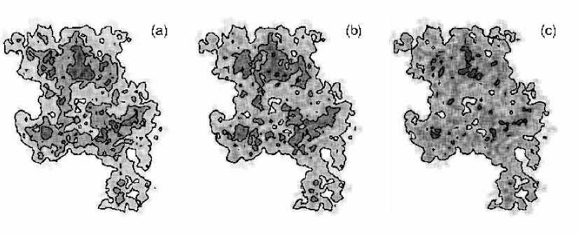
Figure 1: Three images projected of the same cloud with fractal dimension $D_{f}=2.6$ but for three different optical depth values: (a) $\tau_{0}=0$, (b) $\tau_{0}=1$ and (c) $\tau_{0}=2$. The contour levels are fixed at 25%, 50% and 75% of the maximum projected intensity for the case $\tau_{0}=0$.

the total optical depth between the point $(x,y,z)$ and the projection plane. The absorption constant $c$ includes quantities such as the abundance, mean molecular weight and absorption cross-section of the emitting molecule, which we assume constant throughout the structure. For the sake of clarity, we will use the constant $\tau_{0}$: the maximum optical depth in the case in which all the mass ($M_{f}$) is homogeneously distributed throughout the entire available volume ($V_{f}=(4/3)\pi R_{f}^{3}$). Since we have defined $M_{f}=1$ and $R_{f}=1$, we obtain $\tau_{0}=3c/(2\pi)$. As an example, Figure 1 shows three projected images of the same cloud with fractal dimension $D_{f}=2.6$ but for three different maximum optical depth values ($\tau_{0}=0$, $1$ and $2$). The total optical depth is in general a function of the position in the projected map, but its maximum value is always close to $\tau_{0}$. For the example shown the maximum optical depth is $\sim 0.9$ and $\sim 1.7$ when $\tau_{0}=1.0$ and $2.0$, respectively.

As we can note in Figure 1, the main effect of opacity is to shorten the dynamical range of intensity levels as well as to decrease the emission maxima. Here we want to understand how this effect alters the estimation of $D_{f}$. To do this we will use the two estimators used in Paper I: the perimeter-area based dimension ($D_{per}$) and the mass dimension ($D_{m}$). The first method begins fixing a threshold intensity level and defining each object as the set of connected pixels whose intensity value is above this threshold. Then the perimeter and the area of each object in the image is determined and the best linear fit in a log(perimeter)-log(area) plot is calculated. The slope of this fit is $D_{per}/2$ (Mandelbrot, 1983). To increase the number of data points in the linear fit it is useful to take several intensity levels. The second method ($D_{m}$) works by generating random positions along the image and then placing cells of different radii (see details in Paper I). The “mass” of each cell is assumed to be the summed values of all the intensities, and $D_{m}$ is calculated as the slope of the best linear fit in a log(mass)-log(radius) plot. We have run exactly the same algorithms as in Paper I to calculate $D_{per}$ and $D_{m}$ for several random fractal clouds and random projections with different opacities. Our first result is that the mean value of $D_{per}$ is not significantly affected by the cloud opacity. The results for $D_{f}=2.0$, $2.3$ and $2.6$ are shown in Table 1, where we can see that $D_{per}$ stays always within the standard deviation independently of the opacity. For a better understanding of this important result Figure 2 shows, as an example, the log(perimeter)-log(area) plot resulting from using only three intensity levels (0.25, 0.5 and 0.75 times the maximum projected intensity $I_{max}$) for the same fractal cloud shown in Figure 1. Squares in Figure 2 refer to the case $\tau_{0}=0$ and circles to the case $\tau_{0}=1$. For the lowest intensity level ($0.25I_{max}$, denoted as crossed symbols) only one relatively large structure (area $\sim 10^{5}\ pixel^{2}$) is observed, which represents the whole molecular complex. As the threshold intensity is increased, smaller and denser structures which are “embedded” in the complex can be observed (see Figure 1). The central and densest parts (cores) corresponding to a threshold intensity of $0.75I_{max}$ (filled symbols) are difficult to detect for the case $\tau_{0}=1.0$, because opacity occults the internal structure of the densest regions. In contrast, small and low-density regions as well as the gas that lies near the boundaries of the three-dimensional clouds are less affected because they have relatively low column densities. However, the same linear behavior is found for different $\tau_{0}$ values (slopes in Figure 2 are similar within the fit errors) because the ideal monofractal clouds we are simulating keep the same fractal properties at all the spatial scales considered, i.e., the fractal dimension is the same for both large low-density clouds and small high-density cores. This is the reason why the perimeter-area dimension remains almost unchanged. Thus, $D_{per}$ appears as a robust estimator of the fractal dimension given that the shape of the external contour is not modified by opacity, rather it is mainly determined by the internal structure of the cloud. The measure of $D_{per}$ can, in this way, be used to infer the fractal structure of the cloud regardless the opacity of the observed transition line.

The situation is different for the mass dimension because this estimator has to use, unlike $D_{per}$, information from all the cloud structure (mass versus radius) to quantify $D_{m}$, including the internal and dense regions which could be hidden in the projected image due to opacity effects. The results for mass dimension are also shown in Table 1. For the particular case $D_{f}=2.6$ we observe small but significant variations with opacity. The general trend is to increase $D_{m}$ as $\tau_{0}$ increases, an expected result taking into account the fact that higher $\tau_{0}$ values produce maps with shorter dynamical range of intensities. But additionally the errors become higher (worse mass-size correlation) and the method begins to fail (correlation not found) for $\tau_{0}\gtrsim 1.3$.

3 APPLICATION TO MOLECULAR CLOUD MAPS

Considering that opacity almost does not affect the estimation of the perimeter-area dimension for the simulated fractal clouds, we set out to study the fractal dimension of nearby interstellar clouds mapped in different molecular lines. As starting hypothesis, we argue that if different molecules are distributed following very similar patterns then their maps should exhibit nearly the same perimeter-area dimension values, independently of the opacity of the molecular transition line. On the opposite, statistically significant differences will be evidence of internal structure differences. We have used various maps of molecular clouds to calculate both $D_{per}$ and $D_{m}$. We have searched the literature for available similar maps observed in different molecular lines. We first use integrated intensity maps of Ophiuchus and Perseus molecular clouds obtained from the COMPLETE Survey of Star-Forming Regions (Ridge et al., 2006). The maps were obtained from simultaneous observations in the ¹²CO 1-0 and ¹³CO 1-0 transitions at the 14m Five College Radio Astronomy Observatory (FCRAO). The half-power beamwidth (HPBW) is around 45″ for both lines, the data are over-sampled at irregular intervals and they were convolved onto a regular 23″ grid. We have also used integrated intensity maps of Orion molecular cloud obtained from observations with the 45m telescope of the Nobeyama Radio Observatory (Tatematsu et al., 1993). We use three maps of the region around Orion KL in the ¹³CO 1-0, CS 1-0 (observed simultaneously) and C¹⁸O 1-0 transitions. The HPBW was 36″ (for CS) and 15″ (for ¹³CO and C¹⁸O) with a grid spacing of 40″ (CS and ¹³CO) and $\sim$34″ (C¹⁸O). After re-gridding the maps have resolutions of 10″ (CS and ¹³CO) and 17″ (C¹⁸O). In principle, each map provides important information on cloud structure. The high ¹²CO abundance ensures strong emission occurring throughout most of the structure, but the lower-J lines of this molecule are often optically thick providing very little information on the structure of very dense regions within molecular clouds. On the opposite, the lines of lower abundance molecules (such as, for instance, C¹⁸O) are usually optically thin even on multi-parsec scales making them suitable for identifying deep regions, but the emission is limited to the denser gas.

The results are summarized in Figures 3 and 4 which show the perimeter and mass dimensions, respectively, obtained for each of the maps (the bars on the data points are one standard deviation resulting from the best linear fit in the perimeter-area or mass-size log-log plot, see Paper I). The perimeter-area method always gives three-dimensional fractal dimensions in the range $2.6\lesssim D_{f}\lesssim 2.8$ for the Ophiuchus, Perseus and Orion molecular clouds. The exception to this general result was the C¹⁸O map of Orion, which will be discussed in the next section. For each molecular cloud the $D_{per}$ value does not depend, within the error bars, on the transition line used, a behavior which is consistent with the results we found in Section 2. The mass-size method yields $2.5\lesssim D_{f}\lesssim 2.8$ for all the maps (except again the C¹⁸O map), which is in gross agreement with the perimeter-area method. However, here we obtain higher error bars doing more difficult to constraint the range of $D_{f}$ values. Part of this uncertainty is associated with the method itself but part is due to its sensitivity to opacity (Section 2), because opacity variations within each map will affect the looked for correlation. In spite of this limitation, the mass-size method is usefull as an additional and independent tool for verifying values and trends derived from the perimeter-area method, specially in low opacity regions. An example is the relatively low fractal dimension value for the original C¹⁸O map which is obtained from both $D_{per}$ and $D_{m}$, and it will be discussed next.

4 THE EFFECT OF NOISE

The results for the C¹⁸O map of Orion are shown in Figures 3 and 4 as filled circles. The $D_{per}$ value has a higher error bar for the C¹⁸O map of Orion, i.e., there is a worse correlation between the perimeter and the area of the projected clouds. Moreover, the resulting fractal dimension is in the range $D_{f}\simeq 2.3-2.5$, significantly lower than in the other maps. The mass dimension also indicates a relatively low fractal dimension but in this case the value is $D_{f}\simeq 2.0-2.2$. In principle this would imply that the observed structures are more irregular in the C¹⁸O map than in the ¹³CO y CS maps, but two points have to be taken into account before coming to this conclusion. First, the $D_{f}$ values derived from both estimators ($D_{per}$ and $D_{m}$) do not agree. Secondly, if the C¹⁸O map shows mainly dense regions where turbulence is overcome by gravity in order to condense into prestellar cores (Larson, 2005) then the resulting structures should be more regular, i.e., with higher fractal dimension values (Falgarone et al., 2004). Since the C¹⁸O emission is much weaker than the other ones the signal to noise ratio (S/N) is much lower for this map. Vogelaar & Wakker (1994) used Brownian fractals to show that noise distorts the contours and thus tends to increase the estimate of $D_{per}$. This is specially true in maps with low S/N values. Thus, the results $D_{per}\sim 1.4$ and $D_{m}\sim 1.7$ for the C¹⁸O map could be simply due to the fact that very noisy maps produce more irregular structures, and not necessarily meaning that C¹⁸O is distributed in a more irregular pattern in Orion A. In other words, we have to try to disentangle structural aspects from noise effects based only on the two-dimensional projection of the cloud.

In order to test this possibility, we proceeded to increase the S/N ratio by smoothing the maps and then to recalculate the fractal dimensions. We have used a gaussian kernel to convolve the data, where the $\sigma$ of the gaussian determines the size of the neighboring region used to smooth spatial variations. If this variations between neighbor pixels are due, in good part, to noise then the final effect will be some reduction in the image noise level. An optimal algorithm would maximize the S/N ratio throughout the map, such as, for example, the adaptive kernel algorithms do (Lorenz et al., 1993; Ebeling et al., 2006). Here we have used a simple space-invariant gaussian kernel ($\sigma$ constant) and we have calculated $D_{per}$ and $D_{m}$ for different $\sigma$ values. In order to quantify the contrasting quality of the resulting images after smoothing we have introduced a new parameter $C$, named “contrast”, which takes into account the dynamical range of the image and the rms of the background. This parameter is defined as the ratio between the maximum intensity in the map and the standard deviation of the intensity values of the background pixels. The calculation of $D_{per}$ is done by taking a fixed number of brightness levels and finding all the connected pixels (objects) whose brightness values are above each predefined level (Paper I). We consider here as “background” pixels all pixels whose brightness are below the minimum brightness level considered to calculate $D_{per}$ (5% of the maximum brightness in the map). Thus, the parameter $C$ estimates the contrast between the signal of the brightest object in the map and the variations of the background pixels. This parameter would be related to the S/N of the brightest pixel only if the variations of the background pixels are due mainly to noise. We have calculated $C$ for the original maps and for the maps smoothed with different $\sigma$ values. Figure 5 shows the results for the three maps of Orion A used in this work. As expected for a low S/N map, the C¹⁸O map has the lowest contrast, but the interesting result is that this map is the only one that begins increasing $C$ as $\sigma$ increases. This means that as the map is smoothed the rms of the background decreases faster than the peak intensity does. In all the other maps the smoothing of the background variations is accompanied by a decrease of the maximum signal in a higher proportion. The contrast $C$ for the C¹⁸O map exhibits a maximum at $\sigma=1.25$ pixels (see Figure 5). This maximum represents the “optimal” map, in the sense of exhibiting the maximum contrast or, in other words, the minimal noise distorion on the image (in the case that background rms is due mainly to noise). In each case we calculated $D_{per}$ and $D_{m}$ for the smoothed maps and all the results showed the expected behavior, i.e., $D_{per}$ decreases (less irregular boundaries) and $D_{m}$ increases (more homogeneous distribution of intensities) as $\sigma$ increases. Figure 6 shows this result for the C¹⁸O map. For the ¹³CO and CS maps the same behavior could be appreciated for $\sigma\gtrsim 1.5$ whereas for lower $\sigma$ values $D_{per}$ and $D_{m}$ remain more or less constant (within error bars). The perimeter-area based dimension of the C¹⁸O map for the $\sigma$ at which $C$ reaches its maximum value (shown as a vertical line in Figure 6) is $D_{per}=1.31\pm 0.02$ (shown as an open circle in Figure 3), from which it is derived that $D_{f}\simeq 2.7\pm 0.1$, in very good agreement with the results obtained from the ¹³CO and CS maps (Figure 3). In addition, the mass dimension for this case (maximum $C$ value) yields $D_{m}=1.84\pm 0.03$ (open circle in Figure 4) which again is consistent within the error bars with the previous results.

To calculate $D_{per}$ we use a given number of intensity levels in all the range of map intensities (Paper I). In principle we expect that structure information in most of these levels is only slightly distorted by noise in high S/N maps. The lowest levels are probably more affected by noise, but the perimeter dimension is calculated by using all the objects in all the levels and therefore noise affects very little the final result. The opposite occurs in low S/N maps, where most of intensity levels are close to the noise level and cloud boundaries may be artificially lengthened (higher $D_{per}$ values). The smoothing process should correct this problem by flattening the wiggles due to noise in neighboring pixels. But if the image is excessively smoothed the clouds will exhibit unrealistic low $D_{per}$ values. How much does the image have to be smoothed? In high S/N images the distortion produced by noise is minimal, then it is reasonable to impose the condition of maximizing S/N in low S/N maps as a previous step in the estimation of the fractal dimension. While this requirement does not guarantee that the dimension obtained is the “real” one, it does ensure the “best” estimation, diminishing the effect of noise. Since S/N may be an unknown quantity (besides depending on the position in the map) we have looked for a parameter connected to S/N but also easy to calculate for a given map. The contrast $C$ defined in this work equals the S/N of the brightest pixel if the background variations are due to noise. What we are suggesting is that the results obtained when $C$ is maximum are more “realiable” than the results for the original (unsmoothed) map. These arguments are supported by the fact that both estimators ($D_{per}$ and $D_{m}$) approach the same $D_{f}$ value for the C¹⁸O map when $C$ is a maximum, and by the fact that this value agrees with the other map values.

5 CONCLUSIONS

Both the perimeter dimension ($D_{per}$) and the mass dimension ($D_{m}$) are useful tools to infer the three-dimensional structure of molecular clouds from two-dimensional maps. In general, $D_{per}$ yields uncertainties smaller than $D_{m}$, but this last method could be very useful to corroborate values and trends observed in optically thin regions. The opacity does not alter the results derived from the perimeter-area method, but when $\tau\gtrsim 1$ the mass-size method cannot be used in a reliable way to estimate the fractal dimension $D_{f}$. An important point that should be considered when using these methods with real data is that very high noise levels can seriously affect the estimation of $D_{f}$, decreasing artificially its value. One possible strategy to prevent this situation is the use of a smoothing algorithm that maximizes the signal-to-noise ratio (S/N) throughout the map. In this work we have defined a parameter called “contrast” ($C$), which we propose can help to choose the most “reliable” image for estimating $D_{f}$.

From different emission maps of Ophiuchus, Perseus and Orion molecular clouds we obtain that the fractal dimension is always in the range $2.6\lesssim D_{f}\lesssim 2.8$. This result supports our previous suggestion (; ) of a relatively high ($>2.3$) average fractal dimension for the ISM. The ultimate goal is to understand the origin of the ISM structure, therefore it would be important to investigate what physical processes are able to generate high fractal dimension structures.

Table 1: Calculated fractal dimension

Perimeter-area based dimension ($D_{per}$)
$D_{f}$	$\tau_{0}=0.0$	$\tau_{0}=1.0$	$\tau_{0}=2.0$	$\tau_{0}=5.0$
2.0	1.601$\pm$0.024	1.602$\pm$0.021	1.604$\pm$0.021	1.591$\pm$0.019
2.3	1.469$\pm$0.023	1.474$\pm$0.021	1.467$\pm$0.019	1.455$\pm$0.018
2.6	1.359$\pm$0.032	1.364$\pm$0.032	1.367$\pm$0.035	1.359$\pm$0.046
Mass dimension ($D_{m}$)
$D_{f}$	$\tau_{0}=0.0$	$\tau_{0}=0.5$	$\tau_{0}=1.0$	$\tau_{0}=1.25$
2.6	1.808$\pm$0.029	1.816$\pm$0.034	1.876$\pm$0.045	1.860$\pm$0.044

Figure 2: The perimeter as a function of the area for the same fractal cloud shown in Figure 1. Squares (left axis) are for the case $\tau_{0}=0$ and circles (right axis) for $\tau_{0}=1$. The intensity levels are fixed at 25% (crossed symbols), 50% (open symbols) and 75% (filled symbols) of the maximum intensity on the image.

Figure 3: The perimeter dimension $D_{per}$ obtained for each molecular cloud map. The dashed horizontal lines indicate values calculated in Paper I for fractal dimension values $D_{f}$ from 2.0 to 2.9 in increments of 0.1. The open circle refers to the result obtained for the smoothed C¹⁸O map (see text).

Figure 4: The mass dimension $D_{m}$ obtained for each molecular cloud map. The dashed horizontal lines indicate values calculated in Paper I for fractal dimension values $D_{f}$ from 2.0 to 2.9 in increments of 0.1. The open circle refers to the result obtained for the smoothed C¹⁸O map (see text).

Figure 5: The contrast parameter $C$ as a function of the smoothing parameter $\sigma$ for the three maps of Orion A used in this work: ¹³CO (squares), CS (circles) and C¹⁸O (triangles).

Figure 6: The mass dimension (squares) and the perimeter dimension (circles) as a function of the smoothing parameter $\sigma$ for the C¹⁸O map. The dashed vertical line emphasizes the value at which the contrast ($C$) is maximum.

References

- Bazell & Desert (1988) Bazell, D., & Desert, F. X. 1988, ApJ, 333, 353
- Dickman et al. (1990) Dickman, R. L., Horvath, M. A., & Margulis, M. 1990, ApJ, 365, 586
- Ebeling et al. (2006) Ebeling, H., White, D. A., & Rangarajan, F. V. N. 2006, MNRAS, 368, 65
- Elmegreen & Falgarone (1996) Elmegreen, B. G., & Falgarone, E. 1996, ApJ, 471, 816
- Falgarone et al. (1991) Falgarone, E., Phillips, T. G., & Walker, C. K. 1991, ApJ, 378, 186
- Falgarone et al. (2004) Falgarone, E., Hily-Blant, P. , & Levrier, F. 2004, Ap&SS, 292, 89
- Larson (2005) Larson, R. B. 2005, MNRAS, 359, 211
- Lee (2004) Lee, Y. 2004, JKAS, 37, 137
- Lorenz et al. (1993) Lorenz, H., Richter, G. M., Capaccioli, M., & Longo, G. 1993, A&A, 277, 321
- Mandelbrot (1983) Mandelbrot, B. B. 1983, The Fractal Geometry of Nature (New York: Freeman)
- Ridge et al. (2006) Ridge, N. A., et al. 2006, AJ, 131, 2921
- Sánchez et al. (2005) Sánchez, N., Alfaro, E. J., & Pérez, E. 2005, ApJ, 625, 849 (Paper I)
- Sánchez et al. (2006) Sánchez, N., Alfaro, E. J., & Pérez, E. 2006, ApJ, 641, 347 (Paper II)
- Tatematsu et al. (1993) Tatematsu, K. et al. 1993, ApJ, 404, 643
- Vogelaar & Wakker (1994) Vogelaar, M. G. R. & Wakker, B. P. 1994, A&A, 291, 557
- Westpfahl et al. (1999) Westpfahl, D. J., Coleman, P. H., Alexander, J., & Tongue, T. 1999, AJ, 117, 868