PHASE AND INTENSITY DISTRIBUTIONS OF INDIVIDUAL PULSES OF PSR B0950$\boldsymbol{+}$08

Abstract

The distribution of the intensities of individual pulses of PSR B0950$+$08 as a function of the longitudes at which they appear is analyzed. The flux density of the pulsar at 111 MHz varies strongly from day to day (by up to a factor of 13) due to the passage of the radiation through the interstellar plasma (interstellar scintillation). The intensities of individual pulses can exceed the amplitude of the mean pulse profile, obtained by accumulating 770 pulses, by more than an order of magnitude. The intensity distribution along the mean profile is very different for weak and strong pulses. The differential distribution function for the intensities is a power law with index $n={-}1.1\pm 0.06$ up to peak flux densities for individual pulses of the order of 160 Jy.

1 INTRODUCTION

The mean profile obtained by summing several thousand individual pulses is a stable characteristic of a pulsar at a given frequency. In spite of the stability of the mean profile, however, the pulsar’s radiation is very variable on a wide range of time scales: nanoseconds for the giant pulses of the Crab Pulsar [1], tens and hundreds of microseconds for microstructure [2, 3], and several to tens of milliseconds for subpulses in individual pulses. Variability of the amplitude from pulse to pulse and longer-term variability associated with subpulse drift, nulling, and the passage of the radiation through the interstellar plasma (scintillation) is also observed.

We will investigate variations of the amplitudes of subpulses of the mean profile of PSR B0950$+$08 at 111 MHz at various longitudes (phases). The importance of this type of analysis is that different mechanisms used to explain the coherent radio emission of pulsars as being due to plasma microinstabilities or non-linear processes have different electric-field statistics. This parameter is determined by the internal statistics of the radiation in the region of an individual source, effects due to spatial modulation associated with the superposition of the radiation from (possibly) many sources, and effects due to the propagation of the radiation from the source to the observer. The theory of the stochastic growth of plasma instabilities (SGT) [4] predicts a logarithmic normal distribution for variations of the electric field. Non-linear three-wave processes acting in the presence of high electric fields above some critical value $E_{c}$ lead to a power-law distribution with $P(E)\propto E^{-\alpha}$, where $\alpha=4{-}6$. The theory of self-organized criticality (SOC) [5] predicts a power-law distribution with an index close to $\alpha=1$. Analysis of variations in the intensities of individual pulses for the three pulsars PSR B0833-45 [6], B1641-45, and B0950$+$08 [7] showed that their variability corresponds to log-normal field statistics; i.e., it is consistent with the predictions of stochastic-growth theory. We will show below that the variations in the amplitudes of the subpulses of PSR B0950$+$08 at 111 MHz are not consistent with these statistics, and can be described well by a power law.

We chose PSR B0950$+$08 for this analysis because it is one of the most powerful pulsars at meter wavelengths, with a flux density at 102.5 MHz of $S=2$ Jy [8]. This pulsar displays strong linear polarisation at 111 MHz, $P_{l}=(70{-}80)\%$ [9], a weak interpulse located 152^∘ from the main pulse, microstructure with a characteristic time scale of about 150 $\mu$s [3], and low-level extended radiation [10, 11].

2 OBSERVATIONS AND PRELIMINARY REDUCTION OF THE DATA

Our data for PSR B0950$+$08 were obtained at 111.2 MHz on the BSA radio telescope of the Pushchino Radio Astronomy Observatory (Astro Space Center of the Lebedev Physical Institute) in two series of observations, during September 8–October 14, 2001 and August 16–September 10, 2004. Only linear polarization was received. A multi-channel receiver with 64 channels each with a bandwidth of 20 kHz was used. The time for each observing session was 3.3 min, corresponding to an accumulation of 770 individual pulses. The time resolution in the first series of observations was 0.4096 ms, and in the second series 1.28 ms; the receiver time constant was 0.3 and 3 ms in the first and second series, respectively. The dispersion broadening in each 20 kHz channel at the observing frequency was 0.35 ms.

The individual pulses in all channels within a window of 150 ms (first series) or 400 ms (1.6 times the pulsar period; second series) were recorded on a computer disk, synchronous with the pre-calculated topocentric pulse arrival times. The signals were then dispersion-compensated and any channels subject to substantial interference removed. Further, the signals in all channels were added after a preliminary reduction to a single gain via appropriate normalization, such that the dispersions of the noise in all the channels were equal to the value averaged over all the channels. The mean pulse profile for each observing session was obtained by adding all the individual pulses. The mean background determined from a noise interval outside the window of the pulse radiation was subtracted from each pulse, and the rms deviations of the noise level from the mean level in this region were determined, which were then used to calculate the mean $\sigma_{N}$ for the observing session for the individual pulses.

For each observing session, we calculated the peak amplitude $A_{\textrm{max}}$, the signal-to-noise ratio S/N (the ratio of the amplitude of the mean profile to $\sigma_{N}$, derived using a noise interval outside the mean pulse), and the ‘‘energy’’ in the mean pulse, derived by summing the intensities within the mean profile with values $I>4\sigma_{N}$. Our analysis of the individual pulses consisted of determining the positions (phases) and amplitudes of the subpulses within each pulse, which were then used to construct the amplitude distribution functions at various longitudes of the mean pulse.

3 INFLUENCE OF POLARIZATION AND SCINTILLATION

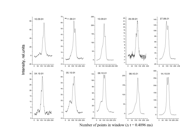
Figure 1: Mean pulse profiles for PSR B0950$+$08 at $f=111.23$ MHz over 10 days in the first series of observations.

Figure 1 presents the mean profiles over 10 days in the first series of observations. This figure clearly shows how strongly the pulse shape and S/N varies from day to day. The profile varies from a well defined three-component pulse (October 6, 2001) to a two-component pulse (October 14, 2001) in which the first component is virtually completely absent. This behavior of the mean pulse reflects the strong influence of the polarization of the received radiation. The analysis of profile variations in PSR B0950$+$08 at frequencies 41–112 MHz carried out in [9] showed that the rotation measure for this pulsar is $\textrm{RM}=4\leavevmode\nobreak\ {\textrm{rad}}/{\textrm{m}^{2}}$. The period of the Faraday modulation at 111.2 MHz is 6 MHz, and the corresponding rotation of the plane of polarization over the receiver bandwidth ($B=1.28$ MHz) is 37^∘. The contribution of the ionosphere to the rotation measure at this frequency is no more than 10%, and can be neglected. The influence of the polarization of the received radiation amounts to variations in the amplitudes of all three components from session to session. The polarization profile at 151 MHz obtained by Lyne et al. [12] shows variations of the polarization angle by 160^∘ along the mean profile, which encompasses the unresolved (in those observations) first component and the two others. Fitting polarization models to the observed frequency variations of the mean-profile components yielded $100\%$, $75\%$, and $80\%$ for the degrees of linear polarization of the first, second and third components, respectively [9]. This means that the amplitude of the first component can vary from zero to its maximum value, the second by a factor of two, and the third by a factor of 2.4 from session to session. Accordingly, we must take this effect into account when analyzing variations in the intensities of subpulses at various longitudes of the mean profile.

PSR B0950$+$08 is one of the most nearby pulsars, at a distance of $R=262$ pc [13] and with a dispersion measure of $\textrm{DM}=2.97\leavevmode\nobreak\ {\textrm{\leavevmode\nobreak\ pc}}/{\textrm{cm}^{3}}$. Accordingly, the pulsar radiation should be strongly modulated by interstellar scintillation. A frequency analysis of our data shows that the characteristic scale for the decorrelation with frequency determined as the half-width of the autocorrelation function (ACF) at the half-maximum level is $\Delta f_{d}$ = 200 kHz. The spectrum does not vary over the observation time; i.e., the characteristic time scale for the scintillations is longer than the observation time, $t_{d}>3.3$ min. The intensity in each spectral channel was determined by averaging the intensities within a longitude interval chosen so that the signal in the mean profile at these longitudes was more than half the maximum amplitude of the mean pulse. We then averaged the spectra of 127 pulses, thus obtaining spectra of the intensity variations every 32.1 s. The characteristic decorrelation scale was determined from the mean ACF derived by averaging the ACFs from spectra obtained over the entire observing session.

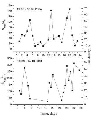
Figure 2: Time dependence of the amplitude of the mean profile in units of $\sigma_{N}$ for the two series of observations. The peak flux-density scale in Jy is indicated to the right.

Figure 2 presents the time dependence of the amplitude of the mean profile $A_{\textrm{max}}$ in units of $\sigma_{N}$ for the two series of observations. We can see the strong variability of this amplitude from day to day due to scintillation. The maximum variations in the value of $A_{\textrm{max}}$ for the mean profile reach a factor of 13. We used the following relation to scale the peak pulse amplitudes for different days in flux-density units (Jy):

$$A_{\textrm{max}}(t)\mbox{\leavevmode\nobreak\ [Jy]}=\frac{A_{\textrm{max}}(t)}{\langle A_{\textrm{max}}\rangle}\cdot S\cdot k_{1},$$ (1)

where $S=2$ Jy is the flux density of the pulsar at our frequency (since $f=111.2$ MHz is close to the frequency of [8], we neglected the frequency dependence $S(f)$), $k_{1}=14.7$ is a coefficient relating the ratio of the peak amplitude to the energy in the pulse averaged over the pulsar period, and $\langle A_{\textrm{max}}\rangle$ is the mean of $A_{\textrm{max}}$ over the entire series of observations in relative units. The energy in the pulse is taken to be the sum of the intensities within the mean profile with values $I>4\sigma_{N}$ multiplied by the time step between points. For example, $A_{\textrm{max}}(t)\mbox{\leavevmode\nobreak\ [Jy]}=A_{\textrm{max}}(t)\cdot 0.187$ for the first and $A_{\textrm{max}}(t)\mbox{\leavevmode\nobreak\ [Jy]}=A_{\textrm{max}}(t)\cdot 0.467$ for the second observation series. The corresponding scale of the peak flux densities $S_{p}$ in Jy is shown to the right in Fig. 2. The mean value of this quantity is $\langle S_{p}\rangle=29.4$ Jy.

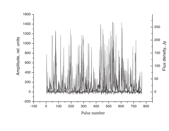
Figure 3: Variations in the amplitudes of individual pulses during the observations of October 11, 2001. The variations of the mean noise amplitude determined outside the emission window for these same pulses is also shown.

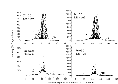
Figure 4: Distribution of the intensities of the individual pulses at various longitudes of the mean pulse for several sessions in the first series of observations. The mean pulse profile for a given session multiplied by the indicated coefficient is also shown, as well as the signal-to-noise ratio S/N for the corresponding mean profiles.

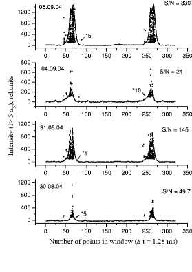
Figure 5: Same as Fig. 4 for the second series of observations.

4 VARIATIONS OF THE INTENSITIES OF INDIVIDUAL PULSES

Figure 3 shows the variations of the indiviual-pulse amplitudes during the observing session on October 11, 2001. The amplitude was taken at the longitude of the maximum of the mean profile. We can clearly see the strong variability of the radiation, whose intensity varies from zero to amplitudes with $\textrm{S/N}\sim 70$. The same figure presents the variations in the noise amplitude outside the pulse-emission window.

Figures 4 and 5 show the longitude distributions of the peak amplitudes of individual pulses over four sessions in the two series of observations. The mean profiles multiplied by the indicated coefficients are also presented. Here, we chose only pulses with amplitudes exceeding $5\sigma_{N}$. We can see three distinguished regions corresponding to the positions of the maxima of the three components of the mean profile, where subpulses appear most often. The maximum pulse amplitudes for sessions with low S/N (here, $\textrm{S/N}=A_{\textrm{max}}/\sigma_{N}$ for the mean profile) exceed the value $A_{\textrm{max}}$ for the mean profile by more than an order of magnitude. For sessions with high S/N (${\sim}$300), the maximum pulse amplitudes are close to $5A_{\textrm{max}}$, while their absolute values are approximately equal to the amplitudes of the strongest pulses for weak records. This reflects the fact that the dynamic range of our analog–digital converter is not sufficient to accurately register the amplitudes of the strongest pulses, so that the amplitudes are cut off when the energy in the pulse grows substantially due to scintillation. Therefore, the real intensities of the strongest pulses are reflected by recordings with low mean-profile amplitudes. We took this effect into account in our subsequent analysis of the data. Note that the peak amplitude of the strongest pulse $S_{p}$ for September 26, 2001 exceeds the amplitude of the mean profile for that session by a factor of 60, which corresponds to $S_{p}\geq 270$ Jy.

5 DISTRIBUTION FUNCTION

The distribution of the number of pulses exceeding a given intensity threshold (for two observing sessions) is presented in the upper part of Fig. 6 on a double-log scale. The intensities of the individual pulses are normalized using $\sigma_{N}$. We used only pulses with amplitudes exceeding $5\sigma_{N}$ to construct this distribution. The mean profiles for the corresponding sessions are also shown. We obtained separate distributions for pulses appearing at the longitudes of the maxima of the first, second, and third components on September 13, 2001 and of the second and third components on October 14, 2001. We can see that the distribution becomes appreciably steeper at high values of $I/\sigma_{N}$, which refects the cut-off of the amplitudes of strong pulses due to the instrumental effect mentioned above. The vertical lines in the figure correspond to the cut-off boundaries, which depend on the S/N of the mean profile for a given session.

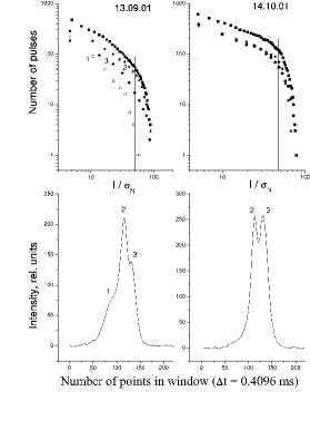
Figure 6: Number of pulses exceeding a specified intensity threshold as a function of the intensity $I$ in units of $\sigma_{N}$ (upper plots) together with the corresponding mean profiles (lower plots). Distributions were constructed separately for pulses appearing at the longitudes of the maxima of the first component (hollow circles), second component (asterisks), and third component (filled circles). The squares show the overall distribution of the pulses independent of the longitude at which they appear.

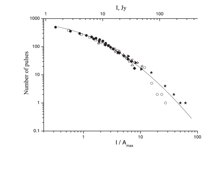
Figure 7: Integral distribution function constructed for eight days of observations. The data for different days are shown by different symbols. A parabola fit to all the points using the least-squares method is also shown.

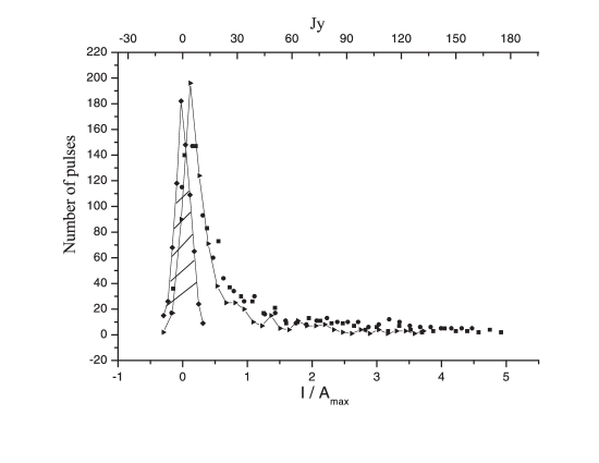
Figure 8: Differential distribution function constructed for the noise (shaded) and the data for three days of observations with high signal-to-noise ratio S/N in the mean profile. The intensity was taken at the longitude of the maximum for the mean profile.

At the longitude of the maximum of the first component, the distribution becomes steeper, only the strongest pulses reach the cut-off boundary, and the distribution correctly reflects the original distribution. At the longitudes of the second and third components, the distributions are similar out to the cut-off boundaries, differing only in a coordinate shift corresponding to the ratio of the amplitudes of these components in the mean profile. On October 14, 2001, the component amplitudes are approximately the same, and the distributions coincide. Since the strong linear polarization of the components leads to substantial variations of their amplitudes in the mean profile, we used the pulse intensities at the longitude of the mean-profile maximum to construct the integral distribution functions using the data for different days of observations. To exclude the effect of scintillation, we normalized the pulse intensities to the amplitude of the mean profile, $A_{\textrm{max}}$.

Figure 7 shows the resulting distributions constructed for eight days of observations, with pulses with amplitudes exceeding the cut-off boundaries excluded. We can see that the data for different days are in very good agreement, testifying that we have correctly removed the indicated instrumental effect and the influence of polarization and scintillation. The distributions presented on a double-log scale are well described by a parabola, and we obtained a parabolic least-squares fit to all the points in the distribution, also shown in Fig. 7: $\log N=2.44-0.77\log(I/A_{\textrm{max}})-0.43\log(I/A_{\textrm{max}})^{2}$.

Figure 8 presents differential distribution functions constructed using the noise (left) and pulse data for three days of observations with high S/N. The intensities of individual pulses were taken at the longitude of the maximum of the mean profile. The noise distribution is Gaussian, with a zero mean and $\sigma$ = 0.07 in units of $I/A_{\textrm{max}}$. When constructing the pulse distribution, the only constraint we applied was excluding high intensities that exceeded the cut-off boundary. The maximum of this distribution is shifted from zero by $x=0.117$. This indicates that there are an appreciable fraction of pulses with small intensities in the radiation of PSR B0950$+$08.

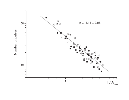
Figure 9: Differential distribution function constructed using data for six days of observations shown on a double-log scale. The intensities were taken at the longitude of the mean-profile maximum. The line is the result of a least-squares fit.

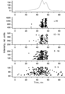
Figure 10: Longitude distribution of the individual pulses with the indicated range of intensities in units of $\sigma_{N}$. The mean profile for October 11, 2001 is shown above.

The differential distribution function for pulses with $I>5\sigma_{N}$ for six days of observations with high S/N is presented in Fig. 9 on a double-log scale. Here, we likewise used only data to the cut-off boundary. A linear least-squares fit to all the points has the slope $n={-}1.11\pm 0.06$ to intensities $I/A_{\textrm{max}}\approx$ 4.5 or 160 Jy. The distributions for days with relatively low signal-to-noise ratios $\textrm{S/N}\approx 30{-}120$, i.e., with appreciably more distant cut-off boundaries, are the steepest: $n={-}1.5\pm 0.2$ for $I>160$ Jy. Although the statistics for pulses with high intensities are relatively poor, it appears that these results confirm a steepening of the distribution function for $I>160$ Jy.

The power-law distribution function $P(I)\sim I^{-n}$ ($n\approx 1$) that we have obtained for the ordinary pulsed radiation of PSR 0950+08 agrees with the predictions of self-organized criticality theory [5]. This theory is based on the idea that there is a self-consistent interaction between waves, the flow of moving particles, and the surrounding plasma, which is near marginal stability. This theory predicts a power-law distribution $P(E^{2})\sim E^{-\beta}$ over a wide range of energies (intensities), with $\beta\approx 1$ and varying from 0.5 to 2 for various systems [5], and the power-law distribution $P(E)\sim E^{-\alpha}$ for the electric field $E=\sqrt{I}$. Here, $\alpha=2\beta-1$ [14], and accordingly $\alpha\approx 3.4$ and $\beta\approx 2.2$ in our case. As was shown in [14], giant pulses and giant micropulses in a number of pulsars display power-law distribution functions with $n=4.4{-}6.5$, appreciably higher than our value $n\approx$ 1. This provides evidence that giant pulses and micropulses are generated by a different process than that giving rise to the normal radiation and/or are formed in a very different region.

The statistics of the 430 MHz pulsed radiation of PSR 0950+08 at various phases of the mean profile was studied by Cairns et al. [7], who showed that the distribution function for the logarithm of the electric field, $P(\log E)$, varies significantly with phase, with the distribution at the longitude of the mean-profile maximum being approximately flat in the range $2.1\leq\log E\leq 2.7$ and falling off in accordance with a power law at $\log E>2.7$ [7, Fig. 22]. This range of $E$ corresponds to their data for $5\sigma_{N}\leq I\leq 75\sigma_{N}$. Cairns et al. [7] fit a combination of a Gaussian intensity distribution and a non-linear log-normal distribution to the distribution they obtained. The statistics for the fit are relatively poor, but it provides a good qualitative description of the data. Since $P(\log E)=2IP(I)$, the distribution we have obtained, $P(I)\sim I^{-1.1}$, corresponds to a flat $P(\log E)$ [7]. We also observe a steepening of $P(I)$ at high intensities. It appears that the distribution of the intensity at the longitude of the mean-profile maximum is described by a piecewise-power-law function.

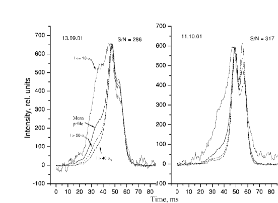
Figure 11: Mean profiles for two days of observations obtained by summing all pulses (solid curve) and pulses with intensities $3\sigma_{N}<I<10\sigma_{N}$ (dotted curve), $I>20\sigma_{N}$ (dashed curve), and $I>40\sigma_{N}$ (dot–dashed curve). The amplitudes of all the profiles (in relative units) have been normalized to a single value.

6 LONGITUDE DISTRIBUTIONS FOR WEAK AND STRONG PULSES

In order to investigate the longitude distributions of pulses with different intensities, we divided the pulses into groups having various intensity ranges: $(3-5)\sigma_{N}$, $(5-10)\sigma_{N}$, $(10-15)\sigma_{N}$, and more than 20$\sigma_{N}$. As we can see in Fig. 10, the weaker the pulses, the broader the range of longitudes in which they appear. The stronger the pulses, the narrower the longitude region in which they appear and the more they are concentrated toward the longitudes of the maximum intensities of the second and third components of the mean profile. An analysis for many sessions indicates that this is a general property of this pulsar that does not depend on the shape of the mean profile.

Figure 11 shows mean profiles obtained by summing pulses with intensities in the ranges indicated in the figure. We can see the dependence of the longitude distribution of the intensities on the intensity of the pulses used in the sum. In the case of the profile obtained by summing weak pulses, the amplitude of the first component relative to the second component grows appreciably, while the amplitude of the third component is decreased. The stronger the pulses that are summed, the lower the contribution of the first component and the greater the amplitude of the third component. This behavior is characteristic of all sessions, and does not depend on the shape of the mean profile obtained by summing all pulses. The width of the profile at the half-maximum level, 0.5$A_{\textrm{max}}$, obtained by summing weak pulses is approximately twice the width of the profiles obtained by summing strong pulses, although the widths at the level 0.1$A_{\textrm{max}}$ are approximately the same. Analysis of the pulse intensities for the second series of observations, when we recorded the pulsar emission in a 400 ms window (1.6 $P_{1}$), showed an absence of pulses with amplitudes exceeding 5$\sigma_{N}$ outside the range of longitudes for the main pulse.

7 CONCLUSION

Our analysis of variations in the pulse intensities for PSR B0950$+$08 has shown the presence of strong variations in the amplitude of the mean profile (by up to a factor of 13) due to diffractive scintillation, whose time scale exceeds the time for individual observations ($T>4$ min). The intensities of individual pulses can exceed the amplitude of the mean profile on individual days by more than an order of magnitude ($I>340$ Jy). Does PSR B0950$+$08 display giant pulses? Although the strongest recorded pulse exceeded the amplitude of the mean profile on that day by a factor of 60, it exceed the mean amplitude for the entire series of observations by only a factor of 9.3. The strongest pulses appear within a narrow range of longitudes near the longitude of the third component, and display a power-law distribution. All of these properties are consistent with the characteristics of giant pulses, although the relative amplitudes of the strongest pulses are appreciably lower than those for the giant pulses of the Crab Pulsar. The question of which pulses should be considered giant pulses remains open, since there is no precise definition for this phenomenon. We also note that searches for giant pulses from weak, nearby pulsars must take into account the influence on the observed flux densities of effects associated with the passage of the radiation through the interstellar plasma. If a pulsar is very weak and its mean profile can be distinguished only after accumulating a large number of pulses, individual pulses may be visible at specific times due to the enhancement of the signal amplitude due to scintillation. These pulses could be erroneously identified as giant pulses when compared with the low amplitude for the mean pulse over a long time interval.

We have investigated the longitude distributions of pulses with differing intensities. In the case of weak pulses, the radiation at the longitude of the first component grows appreciably, while strong pulses are primarily realized at the longitudes of the second and third components of the mean profile. The radiation of both weak and strong pulses probably comes from a single level in the pulsar magnetosphere, since the total widths of their radiation cones, indicated by the widths of their mean profiles at a low level of the profile, are approximately the same. The differential distribution function is well fit by a power law with index $n={-}1.1\pm 0.06$, in agreement with the predictions of SOC theory. There is some evidence that the distribution function becomes steeper for pulse intensities exceeding 160 Jy.

8 ACKNOWLEDGEMENTS

This work was supported by the Russian Foundation for Basic Research (project codes 03-02-16522, 03-02-16509) and the National Science Foundation (grant AST0098685).

References

- (1) T. H. Hankins, J. S. Kern, J. C. Weatherall, and J. A. Eilek, Nature 422, 141 (2003).
- (2) B. J. Rickett, T. H. Hankins, and J. H. Cordes, Astrophys. J. 201, 425 (1975).
- (3) M. V. Popov, T. V. Smirnova, and V. A. Soglasnov, Astron. Zh. 64, 1013 (1987) [Sov. Astron. 31, 529 (1987)].
- (4) P. A. Robinson and I. H. Cairns, Phys. Plasmas 8, 2394 (2001).
- (5) P. Back, C. Tang, and K. Weisenfeld, Phys. Rev. Lett. 59, 381 (1987).
- (6) I. H. Cairns, S. Johnston, and P. Das, Astrophys. J. 563, L65 (2001).
- (7) I. H. Cairns, S. Johnston, and P. Das, Mon. Not. R. Astron. Soc. 353, 270 (2004).
- (8) V. M. Malofeev, O. I. Malov, and N. V. Shchegoleva, Astron. Zh. 77, 499 (2000) [Astron. Rep. 44, 436 (2000)].
- (9) T. V. Shabanova, Yu. P. Shitov, Astron. Astrophys. 418, 203 (2004).
- (10) T. H. Hankins and J. M. Cordes, Astrophys. J. 249, 241 (1981).
- (11) T. V. Smirnova and T. V. Shabanova, Astron. Zh. 65, 117 (1988) [Sov. Astron. 32, 61 (1988)].
- (12) A. G. Lyne, F. G. Smith, and D. A. Graham, Mon. Not. R. Astron. Soc. 153, 337 (1971).
- (13) W. E. Brisken, J. M. Benson, W. M. Goss, and S. E. Thorsett, Astrophys. J. 573, L111 (2002).
- (14) I. H. Cairns, Astrophys. J. 610, 948 (2004).