IC/2006/108
HUTP-06/A0041

  Abstract
We analyze the 3-year WMAP data and look for a deviation from Gaussianity in the form of a 3-point function that has either of the two theoretically motivated shapes: local and equilateral. There is no evidence of departure from Gaussianity and the analysis gives the presently tightest bounds on the parameters $f_{\rm NL}^{\rm local}$ and $f_{\rm NL}^{\rm equil.}$, which define the amplitude of respectively the local and the equilateral non-Gaussianity: $-36<f_{\rm NL}^{\rm local}<100$, $-256<f_{\rm NL}^{\rm equil.}<332$ at 95% C.L.

 

1 Introduction

During the last few years our understanding of primordial non-Gaussianities of cosmological perturbations has improved significantly.

On the theoretical side it has been firmly established [1, 2] that the simplest models of inflation sharply predict a level of non-Gaussianity ($\lesssim 10^{-6}$) far below the detection threshold of foreseable CMB experiments. Non-Gaussianity therefore represents a smoking gun for deviations from this minimal scenario; in fact many alternatives have been studied which give a much larger non-Gaussianity, an incomplete list including [3, 4, 5, 6, 7, 8, 9, 10]. In all these models the deviation from pure Gaussian statistics shows up in the 3-point correlator of density perturbations. This 3-point function contains all the information about deviation from Gaussianity: no additional information to constrain these models can be obtained looking for other signatures of non-Gaussianity, e.g. Minkowski functionals or the 4-point function [11]. Moreover it has been noted that, as every model gives a definite prediction for the dependence of the 3-point function on the 3-momenta, information about the source of non-Gaussianity in the early Universe can be recovered by the study of the shape dependence of the 3-point correlator [12].

From the experimental point of view the progress has been dramatic. The WMAP experiment has greatly tightened the limits on departures from Gaussianity. Given the relative simplicity of the physics describing the CMB, which allows a linearized treatment of perturbations, and the large data set provided by WMAP, this experiment alone gives practically all the information we have about non-Gaussianity nowadays. In [13] the recent 3-year data have been analyzed by the WMAP collaboration; no evidence for non-Gaussianity has been found and new bounds are obtained.

The purpose of this paper is to extend this analysis of WMAP 3 year data, similarly to what was done for the 1 year data release in [14]. The main difference with respect to the WMAP collaboration analysis [13] is that we look for two different shapes of the 3-point function. Instead of concentrating only on the so-called “local” shape, we also do the analysis for the other theoretically motivated shape dependence, dubbed “equilateral”. As explained in [12, 15, 14], it is justified to concentrate on these two possibilities, both because these are quite different (so that a single analysis in not good for both) and because they describe with good approximation all the proposed models producing a high level of non-Gaussianity. Roughly speaking the local shape is typical of multi-field models, while the equilateral one characteristic of single field models. Given one of the two shapes one puts constraints on the overall amplitude of the 3-point function, namely on the two parameters $f_{\rm NL}^{\rm local}$ and $f_{\rm NL}^{\rm equil.}$ [14].

Another relevant difference with respect to [13] is the way we cope with the anisotropies of the noise, which is caused by the fact that some regions of the sky are observed by the satellite more often than others. We use an improved version of the estimator as explained in [14], which allows a $\sim 20\%$ tightening of the limits on $f_{\rm NL}^{\rm local}$.

As this paper is an updated version of [14] we will concentrate (section 2) on the new features of the analysis, referring the reader to the 1st year paper [14] for all the details. The new limits on $f_{\rm NL}^{\rm local}$ and $f_{\rm NL}^{\rm equil.}$ are discussed in section 3 and conclusions are drawn in section 4.

2 Differences with respect to the 1st year analysis

2.1 Introduction of the tilt in the analysis.

As data now favor a deviation from a scale invariant spectrum, the analysis of the 3-point function has been updated to take into account the presence of a non-zero tilt. This is completely straightforward in the case of the local shape; the non-Gaussianity for the Newtonian potential $\Phi$ is generated by a quadratic term which is local in real space

$$\Phi({\bf x})=\Phi_{g}({\bf x})+f_{\rm NL}^{\rm local}(\Phi_{g}^{2}({\bf x})-\langle\Phi_{g}^{2}\rangle)\;,$$ (1)

where $\Phi_{g}$ is a Gaussian variable. In the presence of a non-zero tilt this gives in Fourier space

$$\langle\Phi({\bf k}_{1})\Phi({\bf k}_{2})\Phi({\bf k}_{3})\rangle=(2\pi)^{3}\delta^{3}\big{(}{\bf k}_{1}+{\bf k}_{2}+{\bf k}_{3}\big{)}F(k_{1},k_{2},k_{3})$$ (2)

with

$$F(k_{1},k_{2},k_{3}) = 2f_{\rm NL}^{\rm local}\cdot\left[P(k_{1})P(k_{2})+P(k_{1})P(k_{3})+P(k_{2})P(k_{3})\right]$$

$$= f_{\rm NL}^{\rm local}\cdot 2\Delta_{\Phi}^{2}\cdot\left(\frac{1}{k_{1}^{3-(n_{s}-1)}k_{2}^{3-(n_{s}-1)}}+\frac{1}{k_{1}^{3-(n_{s}-1)}k_{3}^{3-(n_{s}-1)}}+\frac{1}{k_{2}^{3-(n_{s}-1)}k_{3}^{3-(n_{s}-1)}}\right)$$

where $P(k)$ is the power spectrum $\langle\Phi({\bf k}_{1})\Phi({\bf k}_{2})\rangle\equiv(2\pi)^{3}\delta^{3}\big{(}{\bf k}_{1}+{\bf k}_{2}\big{)}P(k_{1})$, with normalization $\Delta_{\Phi}$ and tilt $n_{s}$: $P(k)\equiv\Delta_{\Phi}\cdot k^{-3+(n_{s}-1)}$. We remind the reader that the function $F$ enters in the estimator as:

$${\cal{E}} = \frac{1}{N}\cdot\sum_{l_{i}m_{i}}\int d^{2}\hat{n}\;Y_{l_{1}m_{1}}(\hat{n})Y_{l_{2}m_{2}}(\hat{n})Y_{l_{3}m_{3}}(\hat{n})\int\limits^{\infty}_{0}r^{2}dr\;j_{l_{1}}(k_{1}r)j_{l_{2}}(k_{2}r)j_{l_{3}}(k_{3}r)\;C_{l_{1}}^{-1}C_{l_{2}}^{-1}C_{l_{3}}^{-1}$$ (4)

$$\int\frac{2k^{2}_{1}dk_{1}}{\pi}\frac{2k^{2}_{2}dk_{2}}{\pi}\frac{2k^{2}_{3}dk_{3}}{\pi}F(k_{1},k_{2},k_{3})\Delta^{T}_{l_{1}}(k_{1})\Delta^{T}_{l_{2}}(k_{2})\Delta^{T}_{l_{3}}(k_{3})\;a_{l_{1}m_{1}}a_{l_{2}m_{2}}a_{l_{3}m_{3}}\;,$$

where $\Delta^{T}_{l}(k)$ is the CMB transfer function, and where for simplicity we have neglected the term linear in the data discussed in [14]. It is straightforward to check that the only modification introduced in the analysis is that the function $\beta_{l}(r)$ defined in [16] now depends on the tilt, while the function $\alpha_{l}(r)$ remains unchanged:

$$\alpha_{l}(r) \equiv \frac{2}{\pi}\int_{0}^{+\infty}\!\!\!dk\;k^{2}\,\Delta^{T}_{l}(k)j_{l}(kr)$$ (5)

$$\beta_{l}(r) \equiv \frac{2}{\pi}\int_{0}^{+\infty}\!\!\!dk\;k^{-1+(n_{s}-1)}\,\Delta^{T}_{l}(k)j_{l}(kr)\Delta_{\Phi}\;.$$ (6)

As discussed in [14] the analysis of the equilateral shape is done using a template function $F(k_{1},k_{2},k_{3})$, which is very similar (with few percent corrections) to the different shapes predicted by equilateral models, and at the same time sufficiently simple to make the analysis feasible. For the equilateral case the way to take into account a non-zero tilt is not unique. In models which predict this shape of non-Gaussianity the evolution with scale of the 3-point function is not fixed by the tilt of the spectrum.

For consistency with the local shape we can define new $\gamma_{l}(r)$ and $\delta_{l}(r)$ functions as

$$\gamma_{l}(r) \equiv \frac{2}{\pi}\int_{0}^{+\infty}\!\!\!dk\;k^{1+\frac{1}{3}(n_{s}-1)}\,\Delta^{T}_{l}(k)j_{l}(kr)\Delta_{\Phi}^{1/3}$$ (8)

$$\delta_{l}(r) \equiv \frac{2}{\pi}\int_{0}^{+\infty}\!\!\!dk\;k^{\frac{2}{3}(n_{s}-1)}\,\Delta^{T}_{l}(k)j_{l}(kr)\Delta_{\Phi}^{2/3}\;.$$ (9)

The new template shape will be of the form

$$F = f_{\rm NL}^{\rm equil.}\cdot 6\Delta_{\Phi}^{2}\cdot\left(-\frac{1}{k_{1}^{3-(n_{s}-1)}k_{2}^{3-(n_{s}-1)}}+(2\;perm.)-\frac{2}{(k_{1}k_{2}k_{3})^{2-\frac{2}{3}(n_{s}-1)}}\right.$$ (10)

$$\left.+\frac{1}{k_{1}^{1-\frac{1}{3}(n_{s}-1)}k_{2}^{2-\frac{2}{3}(n_{s}-1)}k_{3}^{3-(n_{s}-1)}}+(5\;perm.)\right)\;.$$

As discussed above we expect that the difference between a given model and this template shape, taking also into account differences in the evolution with scale, to be small. Until a clear detection of non-Gaussianity is found, the use of a single template shape for the whole class of “equilateral models” is justified.

2.2 Improved combination of the maps.

In the non-Gaussianity analysis [17, 13] and [14] the 8 maps at different frequency Q1, Q2, V1, V2, W1, W2, W3 and W4 were combined making a pixel by pixel average weighted by the noise $\sigma_{0}^{2}/N_{\rm obs}$, where $N_{\rm obs}$ is the number of observations of the pixel and $\sigma_{0}$ is a band dependent constant. As the $N_{\rm obs}$ maps are very similar to each other, the procedure amounts to take a pixel-independent combination of the maps, weighted by the average noise. This procedure however is not really optimal because it neglects the effect of the beams: at high $l$ one should give more weight to the $W$ bands as they have the narrowest beam. In other words the optimal procedure is an $l$-dependent combination with signal-to-noise weight [18]. The difference with the naive combination becomes more and more relevant going to higher multipoles, when the effect of the beams is relevant. Thus the improvement becomes more important as time passes and noise reduces, allowing to explore regions of higher $l$. Making a combination in Fourier space has however some disadvantage: given the non-locality of the combination in real space it is not clear how to proceed in masking the contaminated regions of the sky.

We choose to use an intermediate procedure. We combine the maps with a constant coefficient as in the previous analyses, but instead of using the noise as weight, we use a weight based on the signal-to-noise ratio at a given fixed multipole $l_{\rm comb}$. If we choose a very small $l_{\rm comb}$, the signal is the same in all the maps and we are back to a noise weight, which is optimal for the lowest multipoles. On the other hand if $l_{\rm comb}$ is large we are making an optimal combination at high $l$, but not so good at low $l$. We tried many values of $l_{\rm comb}$ to get a result which is as close as possible to the optimal combination. The choice $l_{\rm comb}=235$ turns out to be the best one. We estimated that it improves the limits on the $f_{\rm NL}$ parameters by $\sim 1.4\%$ with respect to the original noise weighting. A very small further improvement, of order $0.4\%$, could be theoretically achieved with the optimal signal-to-noise weighting. Given the problems in dealing with the masking of foregrounds, it is clearly not worthwhile using an $l$-dependent combination. In figure (1) we compare the different ways of combining the maps, showing the effective noise as a function of $l$, compared with the signal. We see that $l_{\rm comb}=235$ gives something very close to optimal.

Figure 1: Effective noise for different combinations of the maps compared with the signal (short-dashed). Optimal signal-to-noise combination (solid); the combination used in the analysis, with $l_{\rm comb}=235$ (dotted); and the noise weighted combination, equivalent to $l_{\rm comb}=0$ (long-dashed) used in the 1st year analysis [14] and in the 3yr analysis by the WMAP collaboration [13].

2.3 Variation of the cosmological parameters.

We use for our analysis the Power Law $\Lambda$CDM Model which gives the best fit to WMAP 3 year data (see Table 2 of [13]). The cosmological parameters are given by: $\Omega_{b}h^{2}=0.0223$, $\Omega_{m}h^{2}=0.128$, $h=0.73$, $\tau=0.092$, $n_{s}=0.958$. The most notable differences with respect to the first year parameters are the drop in the optical depth and the presence of a non-zero tilt of the spectrum.

Let us try to estimate the effect of these changes on the variance of the estimators for the $f_{\rm NL}$ parameters. Roughly speaking the reionization optical depth $\tau$ enters as a multiplicative factor $e^{-\tau}$ in front of the transfer function $\Delta_{l}^{T}(k)$ for $l$ corresponding to scales shorter than the horizon at reionization. In first approximation one can assume that the points on the first peak remain unchanged: as their error is very small the normalization will change to keep the power unchanged there. This means that the reduction of the best fit value for $\tau$ from $\tau=0.17$ to $\tau=0.092$ will be compensated by a decrease in the amplitude of perturbations: $\Delta_{\Phi}$ will decrease by approximately $16\%$. The level of non-Gaussianity of the fluctuations is given by $f_{\rm NL}\cdot\Delta_{\Phi}^{1/2}$, so that a decrease in the amplitude of perturbation will relax the constraints on the $f_{\rm NL}$ parameters. The decrease in the optical depth enlarges the error on the $f_{\rm NL}$ parameters by $\sim 8\%$.

Let us now discuss the effect of the tilt. We can schematize the addition of a red tilt as a reduction of the power $\Delta_{\rm short}$ at scales shorter than the first peak and an enhancement for larger scales ($\Delta_{\rm long}$). What is the effect of this on the limits we can put on the $f_{\rm NL}$ parameters? For the local shape the signal is mostly coming from squeezed triangles in Fourier space, with one side much shorter than the others [12]. The non-Gaussian signal for these triangles goes as $\Delta_{\rm long}\cdot\Delta_{\rm short}$ (see eq. (2.1)), while the error, i.e. the typical value in a realization with pure Gaussian statistics, will go as $\Delta_{\rm long}^{1/2}\cdot\Delta_{\rm short}^{1/2}\cdot\Delta_{\rm short}^{1/2}$. Thus the limits on $f_{\rm NL}^{\rm local}$ will become tighter proportionally to $\Delta_{\rm long}^{1/2}$. For the equilateral shape the signal is coming from equilateral configurations. The contribution from triangles with $l$ smaller than the first peak will have more signal while triangles on shorter scale will have less. There is a mild cancellation between these effects giving a rather small effect in the equilateral case. One can check this intuition with a numerical analysis of the variance of the estimator varying the tilt. Going from a flat spectrum to the value of $n_{s}$ favored by WMAP 3yr data, the constraint on $f_{\rm NL}^{\rm local}$ becomes tighter by 9%, while the one on $f_{\rm NL}^{\rm equil.}$ becomes looser by 5%.

Obviously this way of taking into account the variation in the knowledge of the cosmological parameters is quite naive. One should properly marginalize over all parameters when quoting the final limits on the non-Gaussianity. This would slightly enlarge the allowed range, roughly by an amount comparable to the variation induced by the change of the cosmological parameters discussed above. This approach is numerically very demanding but it will be mandatory if a significant detection of non-Gaussianity will be achieved.

One can put together the variations induced by the change in the cosmological parameters with the reduction of the noise given the additional amount of data, to estimate the final improvement on the allowed range for $f_{\rm NL}$. With a scale invariant signal the noise reduction would give a $\sqrt{3}$ improvement. But this is not a good approximation, both because the transfer function imprints features on the scale invariant primordial spectrum and because the beams cut off the signal at high $l$. A good estimate of the improvement is to look at the multipole where signal and noise intersect, with 1st and 3yr data. The constraints on the non-Gaussianity parameters will scale as $N_{\rm pixels}^{-1/2}\propto l_{\rm max}^{-1}$. The multipole of intersection increases by $\sim 20$%, so that we naively expect a $\sim 20$% reduction of the limits. If one puts this together with the discussion above a $\sim 20$% improvement for $f_{\rm NL}^{\rm local}$ is expected, while the improvement on $f_{\rm NL}^{\rm equil.}$ will be really marginal.

3 Results of the analysis

Aside from the few differences discussed above, the analysis of the 3-year data strictly follows what was done for the 1st year release in [14].

For the local shape analysis, the inhomogeneity of the noise, which reflects the fact that different regions of the sky are observed a different number of times, causes some trouble when one extends the analysis to high $l$ where the noise is relevant. The variance of the naive trilinear estimator, which would be optimal in the presence of rotational invariance, starts increasing at a certain point while including more and more data at short scale (see figure 2). This was already noted by the WMAP collaboration in [17]. A partial solution of the problem was given in [14], with the introduction of an improved estimator. The improvement simply consists in an additional term which is linear in the multipoles $a_{lm}$. We stress that this additional term by construction vanishes on average, independently of the value of $f_{\rm NL}^{\rm local}$. In other words it does not bias the estimator, just reduces its variance. In figure 2 we see that the behavior at high $l$ of the new estimator is greatly improved, with a resulting $\sim 20$% improvement on the limits on $f_{\rm NL}^{\rm local}$. The estimator has minimum variance for $l_{\rm max}=370$, with a standard deviation of $34$. Unfortunately this is not a big improvement with respect to the 1st year analysis which had a standard deviation of $37$. From figure 2 we see that an optimal analysis, which would require the full inversion of the covariance matrix, should be able to further reduce the standard deviation to $25$, a $\sim 25$% improvement with respect to our result.

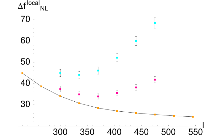
Figure 2: Standard deviation for estimators of $f_{\rm NL}^{\rm local}$ as a function of the maximum $l$ used in the analysis. The combination of the maps is done using $l_{\rm comb}=235$. Lower curve: lower bound deduced from the full sky variance. Lower data points: standard deviation for the trilinear + linear estimator (see details in [14]). Upper data points: the same for the estimator without linear term used in [13]. The error bars are not independent as the results at different $l$ are all based on the same set of MonteCarlo maps.

We applied the estimator to the foreground reduced WMAP sky maps data (see [19] for a discussion about foreground removal) and we obtain $f_{\rm NL}^{\rm local}=32$. There is therefore no evidence of deviation from a Gaussian statistics . The new limits on $f_{\rm NL}^{\rm local}$ are:

$$-36<f_{\rm NL}^{\rm local}<100\quad{\rm at}\;95\%\;{\rm C.L.}$$ (11)

As explained in [14] the effect of the noise inhomogeneities is small for the equilateral shape, so that any improvement of the estimator is useless (see figure 3). Following the discussion in the section above, it is easy to understand that the red tilt makes the curve in figure 3 flatten out faster than in the local case (figure 2): the contribution at high $l$ is suppressed. The estimator does not get worse going to higher $l$ and we can do the analysis at $l_{\rm max}=475$. The standard deviation of the estimator is $147$. As expected the improvement with respect to the first year analysis is marginal, only $\sim 3\%$. The value obtained on the real maps is $f_{\rm NL}^{\rm equil.}=38$. Again there is no evidence of non-Gaussianity of this shape and the new allowed range is given by

$$-256<f_{\rm NL}^{\rm equil.}<332\quad{\rm at}\;95\%\;{\rm C.L.}$$ (12)

An optimal analysis should be able to reduce the range by $\sim 15$% (see figure 3).

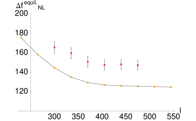
Figure 3: Standard deviation of the estimator of $f_{\rm NL}^{\rm equil.}$ as a function of the maximum $l$ used in the analysis. The combination of the maps is done using $l_{\rm comb}=235$. Lower curve: lower bound deduced from the full sky variance. Data points: standard deviation for the estimator used in the analysis. The error bars are not independent as the results at different $l$ are all based on the same set of MonteCarlo maps.

4 Conclusions

We have analyzed the 3-year WMAP data and looked for theoretically motivated deviations from Gaussianity. Inflationary models which give an observable amount of non-Gaussianity predict a 3-point function of either local or equilateral form. In the data there is no evidence of deviation from Gaussianity, so that we derive bounds on the parameters $f_{\rm NL}^{\rm local}$ and $f_{\rm NL}^{\rm equil.}$, the amplitude of the local and equilateral shape, respectively. The results are

$$-36< f_{\rm NL}^{\rm local} <100\quad{\rm at}\;95\%\;{\rm C.L.}$$ (13)

$$-256< f_{\rm NL}^{\rm equil.} <332\quad{\rm at}\;95\%\;{\rm C.L.}$$ (14)

The improvement with respect to the 1st year analysis is marginal ($\sim 10\%$ in the local case and $\sim 3\%$ for the equilateral case): the expected $\sim 20\%$ improvement from noise reduction is partially compensated by a change in the best fit cosmological parameters. A further $\sim 20\%$ improvement is expected with 8-year statistics. In the future, this kind of analysis will allow to extract in a numerically feasible way almost all the information about $f_{\rm NL}^{\rm local}$ and $f_{\rm NL}^{\rm equil.}$ from Planck data. The signal should be dominant until $l\sim 1500$, so that one expects a factor of 4 improvement. In addition, polarization measurements can further enhance the sensitivity by a factor of 1.6 [20].

We stress that our approach is to look only for forms of non-Gaussianity which are theoretically motivated within the inflationary paradigm. Our results are not in contradiction with some claims in the literature of detection of a non-Gaussian statistics different from ours (see for example [22, 23] and references therein). Given the fact there are infinite ways of deviating from Gaussiannity, it remains difficult to assess the statistical significance of those results.

References

- [1] J. Maldacena, “Non-Gaussian features of primordial fluctuations in single field inflationary models,” JHEP 0305, 013 (2003) [astro-ph/0210603].
- [2] V. Acquaviva, N. Bartolo, S. Matarrese and A. Riotto, “Second-order cosmological perturbations from inflation,” Nucl. Phys. B 667, 119 (2003) [astro-ph/0209156].
- [3] D. H. Lyth, C. Ungarelli and D. Wands, “The primordial density perturbation in the curvaton scenario,” Phys. Rev. D 67, 023503 (2003) [astro-ph/0208055].
- [4] M. Zaldarriaga, “Non-Gaussianities in models with a varying inflaton decay rate,” Phys. Rev. D 69, 043508 (2004) [astro-ph/0306006].
- [5] L. Boubekeur and P. Creminelli, “Right-handed neutrinos as the source of density perturbations,” Phys. Rev. D 73, 103516 (2006) [hep-ph/0602052].
- [6] P. Creminelli, “On non-Gaussianities in single-field inflation,” JCAP 0310, 003 (2003) [astro-ph/0306122].
- [7] N. Arkani-Hamed, P. Creminelli, S. Mukohyama and M. Zaldarriaga, “Ghost inflation,” JCAP 0404, 001 (2004) [hep-th/0312100].
- [8] M. Alishahiha, E. Silverstein and D. Tong, “DBI in the sky,” Phys. Rev. D 70, 123505 (2004) [hep-th/0404084].
- [9] L. Senatore, “Tilted ghost inflation,” Phys. Rev. D 71, 043512 (2005) [astro-ph/0406187].
- [10] X. Chen, M. x. Huang, S. Kachru and G. Shiu, “Observational signatures and non-Gaussianities of general single field inflation,” hep-th/0605045.
- [11] P. Creminelli, L. Senatore and M. Zaldarriaga, “Estimators for local non-Gaussianities,” arXiv:astro-ph/0606001.
- [12] D. Babich, P. Creminelli and M. Zaldarriaga, “The shape of non-Gaussianities,” JCAP 0408, 009 (2004) [astro-ph/0405356].
- [13] D. N. Spergel et al., “Wilkinson Microwave Anisotropy Probe (WMAP) three year results: Implications for cosmology,” astro-ph/0603449.
- [14] P. Creminelli, A. Nicolis, L. Senatore, M. Tegmark and M. Zaldarriaga, “Limits on non-Gaussianities from WMAP data,” JCAP 0605, 004 (2006) [astro-ph/0509029].
- [15] P. Creminelli and M. Zaldarriaga, “Single field consistency relation for the 3-point function,” JCAP 0410, 006 (2004) [astro-ph/0407059].
- [16] E. Komatsu, D. N. Spergel and B. D. Wandelt, “Measuring primordial non-Gaussianity in the cosmic microwave background,” Astrophys. J. 634, 14 (2005) [astro-ph/0305189].
- [17] E. Komatsu et al., “First Year Wilkinson Microwave Anisotropy Probe (WMAP) Observations: Tests of Gaussianity,” Astrophys. J. Suppl. 148, 119 (2003) [astro-ph/0302223].
- [18] M. Tegmark, A. de Oliveira-Costa and A. Hamilton, “A high resolution foreground cleaned CMB map from WMAP,” Phys. Rev. D 68, 123523 (2003) [astro-ph/0302496].
- [19] G. Hinshaw et al., “Three-year Wilkinson Microwave Anisotropy Probe (WMAP) observations: Temperature analysis,” astro-ph/0603451.
- [20] D. Babich and M. Zaldarriaga, “Primordial Bispectrum Information from CMB Polarization,” Phys. Rev. D 70, 083005 (2004) [astro-ph/0408455].
- [21] K. M. Gorski, E. Hivon, A. J. Banday, B. D. Wandelt, F. K. Hansen, M. Reinecke and M. Bartelman, “HEALPix – a Framework for High Resolution Discretization, and Fast Analysis of Data Distributed on the Sphere,” Astrophys. J. 622, 759 (2005) [astro-ph/0409513].
- [22] J. D. McEwen, M. P. Hobson, A. N. Lasenby and D. J. Mortlock, Mon. Not. Roy. Astron. Soc. Lett. 371 (2006) L50 [arXiv:astro-ph/0604305].
- [23] K. Land and J. Magueijo, arXiv:astro-ph/0611518.