Barnes-Evans relations for dwarfs with an application to the determination of distances to cataclysmic variables

Abstract

Context. Barnes-Evans type relations provide an empirical relationship between the surface brightness of stars and their color. They are widely used for measuring the distances to stars of known radii, as the Roche-lobe filling secondaries in cataclysmic variables (CVs).

Aims. The calibration of the surface brightness of field dwarfs of near-solar metalicity with spectral types A0 to L8 covers all secondary spectral types detectable in CVs and related objects and will aid in the measurement of their distances.

Methods. The calibrations are based on the radii of field dwarfs measured by the Infrared Flux Method and by interferometry. Published photometry is used and homogenized to the Cousins $R_{\rm c}$ and $I_{\rm c}$ and the CIT $JHK$ photometric systems. The narrow band surface brightness at 7500Å is based on our own and published spectrophotometry. Care is taken to select the dwarfs for near-solar metalicity, appropriate to CVs, and to avoid errors caused by unrecognized binarity.

Results. Relations are provided for the surface brightness in $V$, $R_{\rm c}$, $I_{\rm c}$, $J$, $H$, $K$ and in a narrow band at 7500Å as functions of $V$–$K$ and of spectral type. The method is tested with selected CVs for which independent information on their distances is available. The observed spread in the radii of early M-dwarfs of given mass or luminosity and its influence on the distance measurements of CVs is discussed.

Conclusions. As long as accurate trigonometric parallaxes are not routinely available for a large number of CVs, the surface brightness method remains a reliable means of determining distances to CVs in which a spectral signature of the secondary star can be discerned.

1 Introduction

The spectral flux $F_{\lambda}$ leaving the stellar surface is related to the extinction corrected observed flux $f_{\lambda}$ at the Earth via $F_{\lambda}/f_{\lambda}=(d/R)^{2}$, with $d$ and $R$ the distance and the stellar radius, respectively. On a magnitude scale, $F_{\lambda}$ is referred to as the surface brightness,

$$S_{\lambda} = -2.5\,\mathrm{log}(F_{\lambda}/f_{0})+\mathrm{const}\equiv M_{\lambda}+5\,\mathrm{log}(R/R_{\odot})$$ (1)

$$= m_{\lambda}+5\,\mathrm{log}(R/R_{\odot})-5\,{\rm log}(d/10\,{\rm pc})$$ (2)

$$= m_{\lambda}+5\,\mathrm{log}\phi_{\mathrm{m}as}+0.1564\;,$$ (3)

with $f_{0}$ the flux constant at wavelength $\lambda$ for zero magnitude, $m_{\lambda}=-2.5\,\mathrm{log}(f_{\lambda}/f_{0})$ the extinction-corrected apparent magnitude, $M_{\lambda}$ the absolute magnitude, $R_{\odot}$ the solar radius, and $\phi_{\rm mas}$ the stellar angular diameter in mas. Theoretically, $F_{\lambda}$ is a function of the effective temperature of the star with some dependence also on metalicity and on gravity. This is the physical basis for the empirical calibration of the surface brightness of stars with measured angular diameters as a function of color (Barnes & Evans 1976, Bailey 1981, Ramseyer 1994, Nordgren et al. 2002). Such a calibration allows to determine the radius of a star of known distance and vice versa. The dependencies on metalicity and gravity are clearly discernible in the data (Beuermann et al. 1999) and were not properly taken into account in the earlier calibrations of $S_{\lambda}$ based on supergiants and applied to dwarfs (Bailey 1981, Ramseyer 1994).

The surface brightness method is one of the principal avenues for measuring distances to cataclysmic variables, binaries in which the radius of the Roche-lobe filling dwarf secondary star is reasonably well known from Roche geometry. Clearly, trigonometric parallaxes are to be preferred, but are presently available only for few CVs (Harrison et al. 1999, 2000, 2004a, McArthur et al. 1999, 2001, Monet et al. 2003, Thorstensen 2003, Beuermann et al. 2003, 2004). The secondaries in CVs are characterized by a generally high level of metalicity which we refer to loosely as ‘near-solar’ (Beuermann et al. 1998). Note that the abundances of individual elements may deviate from solar. In this paper, I present new calibrations of the surface brightness of main sequence dwarfs with metalicities similar to those of CV secondaries. They supplement the relations derived for giants, which are used in other fields of research (e.g. Nordgren et al. 2002). I discuss the strengths and fallacies of the photometric/spectrophotometric methods for measuring the distances to CVs using selected objects for which independent distance information is available.

2 General approach

The establishment of a surface brightness vs. color relation requires a set of stars of known angular radii. In this Section, I discuss measured radii of dwarfs and compare them with the theoretical radii of Baraffe et al. (1998, henceforth BCAH). The comparison is made in the absolute magnitude–radius plane rather than in the mass–radius plane since the mass does not enter the present approach. The selection criteria of the stars used in the calibration are subsequently explained and the stellar samples presented.

2.1 Observed and theoretical radii of dwarfs

Measured radii of dwarfs are available from three methods: (i) the Infrared flux method (IRFM) (Shallis & Blackwell 1980, Blackwell & Lynas-Gray, 1994, 1998, and references therein); (ii) long baseline interferometry (Lane et al. 2001, Ségransan et al. 2003, Berger et al. 2006); and (iii) from light curve analyses of eclipsing binaries (Lacy 1977, Torres & Ribas 2002, Ribas 2003, López-Morales & Ribas 2005).

The IRFM, pioneered by Blackwell and collaborators (Shallis & Blackwell 1980, Blackwell & Lynas-Gray, 1994, 1998, and references therein), has yielded accurate radii for a large number of dwarfs and giants. This method derives $T_{\rm eff}$, and $\phi$ from measurements of the wavelength-integrated flux and the spectral flux in a suitable infrared band, using model atmosphere theory in the process. Nordgren et al. (2001) have demonstrated that the IRFM yields angular radii of giants and supergiants which agree with interferometric radii at the 1.4% level. A direct comparison of the IRFM radii of the dwarfs Vega, Sirius A, and Atair with the interferometric radii of Mozurkewich et al. (2003), yields a ratio of IRFM vs. interferometric radii of $1.011\pm 0.037$. Hence, the two methods do, in fact, yield identical results also for dwarfs.

Figure 1: Comparison of observed and calculated radii of dwarf stars vs. absolute magnitude $M_{\rm K}$ in the $K$-band. The solid symbols indicate radii of dwarfs with near-solar abundances (see text) determined by the infrared flux method, open symbols are for old disk/halo stars with metalicities [M/H] = –0.5 to –2. The Sun is indicated by the symbol $\odot$. Crosses refer to interferometrically measured radii of dwarfs which have metalicities between +0.2 and –0.5 and in one case –1.0 (Gl 191, $M_{\rm K}$=7.08). Crossed lozenges indicate the mean components of the four binaries named in the figure. Errors are shown if they exceed the size of the symbols. The theoretical radii are form Baraffe et al. (1998) for an age of 10 Gyrs and metalicities [M/H] = 0 (solid curve) and –1 (dashed curve).

Figure 1 shows the radii of the Sun and twelve dwarfs from Blackwell & Lynas-Gray (1994, 1998) with spectral types between G5 and K6 and metalicities between [M/H] = –0.50 and +0.03  plotted vs. their absolute $K$-band magnitude $M_{\rm K}$ (solid dots with $M_{\mathrm{K}}<5$). They are seen to agree excellently with the theoretical radii of Baraffe et al. (1998) for an age of 1–10 Gyrs and metalicity close to zero or slighly negative. Application of the IRFM to M-stars is more problematic because of the increased structure in their infrared spectra and remaining uncertainties in the theory. Leggett et al. (1996) have applied a variant of the method to 16 M-dwarfs with well-measured parallaxes of which eight are young disk stars with near-solar metalicities and further eight have [M/H] = –0.4 to –2.0 (Fig. 1, solid and open lozenges, respectively). On the average, the radii of the former exceed the BCAH radii by only 2% (Beuermann et al. 1998, 1999), while the metal poor dwarfs seem to have radii on the average about 10% larger than predicted for their luminosity.

The most direct method to measure stellar radii is interferometry. Lane et al. (2001), Ségransan et al. (2003), and Berger et al. (2006) have reported radii of 14 dwarfs with spectral types K3 to M5.5 of which 13 have metalicities between –0.46 and +0.25 and one is a subdwarf with [M/H] = –1.0 (Gl 191). Their results are added to Fig. 1 as crosses, where the sizes of the vertical bars indicate the 1-$\sigma$ errors. Of the 14 stars, the interferometric radii of nine are close to the BCAH [M/H] = 0 model radii, while for five the interferometric radii are larger by some 20%. These are Gl 205, Gl 514, Gl 687, Gl 752A, and Gl 880 with metalicities of +0.21, –0.27, +0.11, –0.05, and –0.04, respectively, which average to solar. There are no systematic differences between the radii determined by the different methods or between the interferometric results of different authors. In particular, the IRFM and interferometric radii of three dwarfs observed with both methods agree within their errors and are also close to the theoretical BCAH radii as exemplified in Tab. 1. The combined interferometric and the IRFM results demonstrate that there is no simple relation between radius excess and metalicity. The fact that some stars have substantially larger radii than suggested by the models is also supported by the radii of dwarfs in binaries shown as crossed lozenges in Fig. 1. Although the effect is highly significant for the mean components in YY Gem (Torres & Ribas 2002) and CM Dra (Metcalfe et al. 1996, Lacy 1977), the absolute differences are only of the order of 10% (Chabrier & Baraffe 1995). Larger effects are found in the binaries GU Boo (López-Morales & Ribas 2005) and CU Cnc (GJ 2069Aab, Ribas 2003).

Table 1: Comparison of the radii of late-type dwarfs measured by the Infrared Flux Method and by interferometry with the theoretical radii of Baraffe et al. (1998) for an age of 10 Gyr and the oberved metalicity. The errors in the observed values are quoted below the appropriate digits.

Name	SpT	$[M/H]\,^{1}$	$M_{\rm K}$	$R/R_{\odot}$
				IRFM$\,{}^{2}$	Interf$\,{}^{3}_{.}$	BCAH$\,{}^{4}$
Gl 105A	K3V	$-0.19$	4.08	0.779	0.708	0.787
		7		39	50
Gl 411	M1.5V	$-0.42$	6.33	0.399	0.393	0.365
		7		12	8
Gl 699	M4V	$-0.5$	8.19	0.194	0.196	0.176
				12	8

¹ From Bonfils et al. (2005) and Leggett et al. (1996).
² From Lane et al. (2001) and Ségransan et al. (2003).
³ From Blackwell & Lynas-Gray (1998) and Leggett et al. (1996).
⁴ From Baraffe et al. (1998), interpolated in $M_{\rm K}$ and $[M/H]$.

In summary, there is a sequence of stars with spectral types A0 to M6.5 and near-solar metalicities which have radii within a few percent of the BCAH [M/H] = 0 model. In addition there is a spread in radius of early M-dwarfs that is not obviously related to differences in metalicity. Unrecognized duplicity can not be the cause for the increased radii of some stars, because duplicity shifts the position of a star in the $R$($M_{\rm K}$) diagram approximately parallel to the theoretical curve, at least at intermediate $M_{\rm K}$. A plausible explanation would be an expansion of the star due to star spots blocking the radiative flux over part of its surface, plausible because the stars in some of the binaries are known to possess large spots (Torres & Ribas 2002, López-Morales & Ribas 2005). Also, the K-star in V471 Tau seems to have a radius $\sim 18$% larger than field K-dwarfs due to star spots (O’Brien et al. 2001). While it is true that the stars showing the largest radius excesses in Fig. 1, Gl 205 ($M_{\rm K}$=5.09), Gl 514 ($M_{\rm K}$=5.67), Gl 752A ($M_{\rm K}$=5.83), and Gl 880 ($M_{\rm K}$=5.35), are not particularly active, spottedness nevertheless seems a more likely cause of the increased radii than an abundance effect since there is no reason for the latter to be prominent only in early M-dwarfs. Another possible cause might be the influence of magnetic fields on convection (Mullan & MacDonald 2001).

A comparison between observed and theoretical radii is obviously complicated by the spread in radii whatever the reason. Tentatively, I consider spottedness as the cause of the increased radii of stars of a given luminosity and effective temperature and, in what follows, I use the term ’immaculate’ for dwarfs with near-solar metalicities which have radii near the theoretical ones (solid curve) in Fig. 1, irrespective of whether they are really spotless or not. Below, I shall derive the surface brightness for immaculate stars as a function of color or spectral type. In applying this relation to derive distances, the possibility of increased radii of ’spotted’ stars has to be specifically taken into account. For immaculate stars of near-solar metalicity, I adopt the numerically available theoretical magnitude-radius relation of Baraffe et al. (1998) for an age of 10 Gyrs and [M/H] = 0, $R_{\mathrm{BCAH}}(M_{\mathrm{K}})$, with a 2% correction in the normalization (Beuermann et al. 1998, 1999) derived from the eight young disk M-dwarfs of Leggett et al. (1996)

$$R(M_{\mathrm{K}})=1.02\,R_{\mathrm{BCAH}}(M_{\mathrm{K}}).$$ (4)

This relation is shown as solid curve in Fig. 1  and allows to estimate the radii of immaculate dwarfs of spectral type late M or L which presently have no measured radii. $R_{\mathrm{BCAH}}(M_{\mathrm{K}})$ is valid down to $M_{\mathrm{K}}\simeq 11$ and yields a nearly constant stellar radius $R\simeq R_{\rm Jupiter}$ for still fainter objects. Its use for field L-dwarfs may not be appropriate in individual cases and the so-derived Barnes-Evans type relations should be considered as preliminary in the L-dwarf regime.

2.2 Specific approach

The Barnes-Evans relations derived here are based on the measured radii of dwarfs with spectral types A0 to M6.5 and near-solar metalicities and refer to immaculate (spotless) stars as discussed in the last Section. Since the latest dwarfs with measured radii are Gl 551 (M5.5, interferometric) and G51-15 (M6.5, IRFM), I add dwarfs from the list of single M-dwarfs of Henry & McCarthy (1996) having $V-K>6.0$ (spectral type dM5+ or later) and from the list of late M and L-dwarfs with measured parallaxes of Dahn et al. (2002). For these stars, the radii are estimated from Eq. (4) and the angular radii follow from the well-known parallaxes. Metalicities are taken from Cayrel de Strobel et al. (2001) or Bonfils et al. (2005) or estimated from the position of the (single) star in the color-magnitude diagram.

The effect of the observed spread in the radii of early M-dwarfs on the surface brightness is included in the Fig. 2, but is omitted in the later figures and the polynomial fits are representative of immaculate stars.

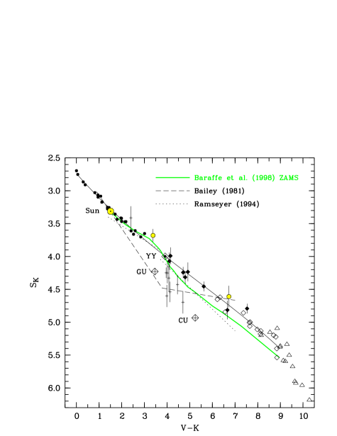
Figure 2: Surface brightness $S_{\rm K}$ in the $K$-band vs. $V$–$K$ for dwarfs of near-solar metalicity. Also shown is the fit from Eq. (5) (solid line), the theoretical relation of BCAH for stars of solar metalicity aged 10 Gyrs (thick green/gray line), and the relations given by Bailey (1981) (dashed) and by Ramseyer (1994) (dotted). The subsamples included in the fit are indicated by different symbols: dwarfs from Blackwell & Lynas-Gray (1994,1998) plus Vega and Sirius (solid circles); the Sun ($\odot$); interferometric radii from Lane et al. (2001) (open circles with error bars); YD dwarfs from Leggett et al. (1996) (filled lozenges); YY Gem $\overline{\rm AB}$ (dotted lozenge), M-dwarfs from Henry & McCarthy (1993) (open lozenges); M/L-dwarfs from Dahn et al. (2002) (open triangles). Shown for comparison, but not included in the fit, are the stars with interferometric radii (crosses) and the binaries (crossed lozenges) from Fig. 1 with near-solar metalicity.

2.3 Photometric stellar sample

The sample of 38 single dwarfs with near-solar metalicity and measured radii includes the following subsamples: (i) 15 dwarfs of spectral class A0 – K1 from Blackwell & Lynas-Gray (1994), supplemented with 9 K-stars from the list of ISO calibration stars (Blackwell & Lynas-Gray 1998) plus Vega and Sirius (Shallis & Blackwell 1980, Mozurkewich et al. 2003); (ii) the Sun; (iii) the mean component of YY Gem (Torres & Ribas 2002); (iv) eight young disk M-dwarfs from Leggett et al. (1996); and (v) Gl 380 and Gl 551 as bona-fide immaculate stars with interferometric radii. This sample is supplemented by (vi) 10 additional M-dwarfs with $V-K>6.0$ from the list of single stars of Henry & McCarthy (1993); and (vii) 36 dwarfs of spectral type M7.5 – L8 from the list of Dahn et al. (2002) with radii computed from Eq. (4). These supplementary stars define the faint end of the Barnes-Evans relations. Care has been taken to avoid unrecognized binaries. The subsample includes both individual components of the binaries LHS2397a, Gl569B, 2M0746+20, and Kelu1, the brighter (L6) component of 2M0850+10, as well as the mean components of DEN0205-11 and DEN1228-15. We can not entirely exclude that a few more binaries lurk behind relatively bright stars of the sample or that particular youth of individual objects affects the results. All photometric data are on the Cousins $R_{\rm c}$, $I_{\rm c}$ and the CIT $JHK$ systems. Much of the $VR_{\mathrm{c}}I_{\mathrm{c}}JHK$ photometry has been taken from Leggett (1992), supplemented by more recent data. Blackwell’s $K$-band photometry in the Johnson system has been converted to CIT using the transformation given by Bessel & Brett (1988). The total sample thus consists of 38 stars of spectral type A0 to M6.5 which have measured radii and are referred to as prime calibrators, supplemented by 50 stars of spectral types M5 to L8 with radii from Eq. (4). Some of the L-stars have no measured $V$-magnitude and are missing in the calibration of the surface brightness vs. $V$–$K$. They are contained, however, in the corresponding calibration vs. spectral type.

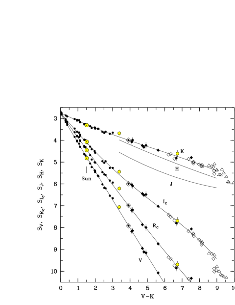
Figure 3: Surface brightness $S_{\rm K}$, $S_{\rm H}$, sj, $S_{\rm I_{\rm c}}$, $S_{\rm R_{\rm c}}$, and $S_{\rm V}$ for immaculate dwarfs with near-solar metalicity. The symbols are the same as in Fig. 2. The fits for the bands $K$, $I_{\rm c}$, $R_{\rm c}$, and $V$ are from Tab. 1, lines 1–4. For completeness the fits for CIT J and H are included, but the data omitted to avoid overlap (see text and Tab. 2).

Figure 4: Surface brightness $S_{\rm K}$, $S_{\rm H}$, $S_{\rm J}$, $S_{\rm I_{\rm c}}$, $S_{\rm R_{\rm c}}$, and $S_{\rm V}$ for immaculate dwarfs with near-solar metalicity vs. spectral type. The symbols are the same as in Fig. 2. The fits are from Tab. 1, lines 5–15. Note that M0 follows K7. For completeness the fits for CIT J and H are included, but the data omitted to avoid overlap (see text and Tab. 2).

Table 2: Parameters of least-squares fits of surface brightness vs. $V$–$K$ or spectral type (see text and footnote on the title page).

(1)	(2)	(3)	(4)			(4)		(5)	(6)	(7)	(8)	(9)	(10)
Line	Dep.	Indep.	Range of			SpT		$a_{0}$	$a_{1}$	$a_{2}$	$a_{3}$	$a_{4}$	$a_{5}$
	Var.	Variable	Ind.Var.			from	to
1	$S_{\rm K}$	$V$–$K$	0	–	8.5	A0	M8	2.739	0.39318	$-0.024337$	$0.00150594$
2	$S_{\rm I_{\rm c}}$	$V$–$K$	0	–	8.5	A0	M8	2.735	0.96065	$-0.026441$	$-0.00455350$	$5.36349\,10^{-4}$
3	$S_{\rm R_{\rm c}}$	$V$–$K$	0	–	8.5	A0	M8	2.750	1.13296	$-0.011563$	$-0.00020917$
4	$S_{\rm V}$	$V$–$K$	0	–	8.5	A0	M8	2.777	1.33603	$-0.006106$
5	$S_{\rm K}$	$X$	58	–	21	A0	K7	9.523	$-0.68789$	0.032091	$-0.00076551$	$9.08518\leavevmode\nobreak\ 10^{-6}$	$-4.31289\leavevmode\nobreak\ 10^{-8}$
6	$S_{\rm K}$	$X$	21	–	13.5	K7	M6.5	17.175	$-1.73019$	0.078260	$-0.00125491$
7	$S_{\rm K}$	$X$	13.5	–	2	M6.5	L8	9.651	$-0.88541$	0.068535	$-0.00211177$
8	$S_{\rm I_{\rm c}}$	$X$	58	–	21	A0	K7	19.534	$-1.49122$	0.060071	$-0.00124465$	$1.29388\leavevmode\nobreak\ 10^{-5}$	$-5.47581\leavevmode\nobreak\ 10^{-8}$
9	$S_{\rm I_{\rm c}}$	$X$	21	–	14	K7	M6	36.892	$-3.90214$	0.164778	$-0.00239313$
10	$S_{\rm I_{\rm c}}$	$X$	14	–	6	M6	L4	14.311	$-0.73014$	0.061393	$-0.00294611$
11	$S_{\rm R_{\rm c}}$	$X$	58	–	21	A0	K7	37.781	$-3.79580$	0.178183	$-0.00422544$	$4.97703\leavevmode\nobreak\ 10^{-5}$	$-2.33252\leavevmode\nobreak\ 10^{-7}$
12	$S_{\rm R_{\rm c}}$	$X$	21	–	14	K7	M6	75.285	$-9.65487$	0.466505	$-0.00777256$
13	$S_{\rm R_{\rm c}}$	$X$	14	–	6	M6	L4	19.916	$-1.83017$	0.177753	$-0.00690745$
14	$S_{\rm V}$	$X$	58	–	21	A0	K7	58.160	$-6.16978$	0.288325	$-0.00671549$	$7.71455\leavevmode\nobreak\ 10^{-5}$	$-3.50806\leavevmode\nobreak\ 10^{-7}$
15	$S_{\rm V}$	$X$	21	–	14	K7	M6	94.817	$-12.2938$	0.592793	$-0.00982453$
16	$F_{7500}$	$X$	48	–	37	A0	K1	$-284.141$	24.7680	$-0.656394$	0.00649903
17	$F_{7500}$	$X$	36	–	16	K1	M4	60.251	$-9.99437$	0.513712	$-0.00665634$
18	$F_{7500}$	$X$	16	–	9	M4+	M9.5	$-21.130$	6.27287	$-0.620218$	0.02054700
19	$F_{TiO}$	$X$	21	–	15	K6	M4.5	$-193.229$	29.87220	$-1.487030$	0.02411810
20	$F_{TiO}$	$X$	15	–	9	M4.5	M9.5	$-1.977$	0.99973	$-0.140786$	0.00610879

2.4 Spectrophotometric stellar sample

The secondary stars in many CVs are detected by their TiO bands in the red part of the spectrum. The derivation of their distances is aided by the calibration of the narrow-band surface brightness in the quasi continuum at 7500Å. Specifically, I consider (i) the mean flux between 7450 and 7550Å and the flux depression below the quasi-continuum at 7165Å, measured by the flux difference in the bands 7450–7550Å and 7140–7190Å (see Fig. 5a below) corrected for atmospheric absorption. This sample is a mixed bag of stars of which we have acquired low-resolution spectrophotometry over the years. All spectrophotometry is readjusted by second degree polynomials in wavelength to force agreement with the measured photometric B, V, $R_{\rm c}$, and $I_{\rm c}$ magnitudes.

The spectrophotometric sample contains a total of 29 K6–L1 dwarfs, of which 15 are common with the photometric sample and of these six have measured radii. Of the remaining 14, eight are from the Henry & McCarthy list of single stars with $V-K<6$ and spectral types K7 to M4+. The radii of all dwarfs without directly measured radii are from Eq. (4). The complete sample contains four known binaries (Gl65, Gl268, Gl473, Gl831) and one triple (Gl866). Their spectral fluxes have been carefully reduced to that of the mean or the dominant single component. One (Gl182) may be a binary based on the brightness criterion and has been tentatively treated as such.

For the calibration of the surface brightness at 7500Å, the genuine spectrophotometry of the 29 K6–L1 dwarfs has been supplemented by synthetic 7500 Å fluxes of the Blackwell et al. A0–K6 dwarfs with measured radii, Gl 380 with an interferometric radius, and the mean component of the binary YY Gem making use of the spectral energy distributions of dwarfs from Silva & Cornell (1992) for the respective spectral type adjusted to the measured $R_{\rm c}$ and $I_{\rm c}$ fluxes.

3 Results

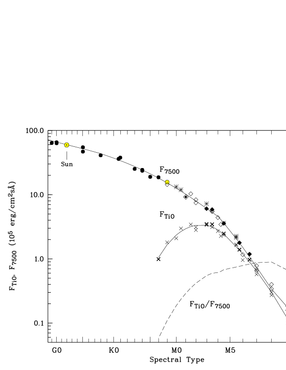
Figure 5: Left: Spectral flux $F_{\lambda}$ at the stellar surface for dwarfs of spectral types K7 to M9. The vertical dotted lines define the intervals over which the quasi-continuum at 7500 Å and the flux deficit at 7165 Å, $F_{7500}$ and $F_{\rm TiO}$, are averaged. Right: Surface brightness of immaculate dwarfs with near-solar metalicity at 7500 Å. Symbols are as in Fig. 2. The data points include additional stars from the Henry & McCarthy (1993) sample of single stars (open lozenges) and the remaining stars from our spectrophotometric sample (asterisks). Also shown is the flux deficit $F_{\rm TiO}$ vs. SpT (lying crosses, lower solid curve). The curves represent the fits from Tab. 2, lines 16–20.

Figure 2 shows the surface brightness $S_{\rm K}$ in the $K$-band vs. $V$–$K$, with $V$–$K$ chosen as independent variable because it correlates well with spectral type and facilitates comparison with the results of Bailey (1981) and Ramseyer (1994). All data with $V$–$K$$<8.2$ can be fitted by a third degree ($n=3$) polynomial

$$S_{\rm K}=\sum_{\mathrm{m}=0}^{\mathrm{n}}a_{\mathrm{m}}(V-K)^{\mathrm{m}}\\$$ (5)

which turns out to be nearly linear (solid black curve). The coefficients $a_{\mathrm{m}}$ are given in Tab. 2, line 1. The residuals from the fit have a standard deviation $\sigma=0.034$ mag for the 27 prime calibrators of spectral type A0–K6, $\sigma=0.094$ mag for the eleven prime calibrators of spectral types K7–M6.5, and $\sigma=0.058$ mag for all 49 stars with $V-K<8.2$ contained in the fit. Included for comparison are the theoretical $S_{\rm K}$($V$–$K$) relation of BCAH for ZAMS stars with solar metalicity (thick green/gray curve) and the results of Bailey (1981) and Ramseyer (1994). The present data agree almost perfectly with the BCAH curve for $V-K<4$ demonstrating the excellent internal agreement between the stellar radii provided by the IRFM and the theoretical stellar radii of Baraffe et al. (1998). The theoretical curve displays some hump structure around $V-K\simeq 3$ which is also visible in the data, but is not accounted for by the low-degree polynomial fit of Eq. (5). The divergence between the data and the BCAH curve at larger $V$–$K$ is a known artefact on the theoretical side caused by the synthetic $V$-magnitudes of the late-type stellar models coming out too bright and $V$–$K$ correspondingly too small (I. Baraffe, private communication). The fit of Fig. 2 is a substantial improvement over the widely used results of Bailey (1981) and Ramseyer (1994) based on supergiants. The mean component of the binary YY Gem falls right on the fit of Eq. (5), while GU Boo, CU Cnc, and the dwarfs with interferometrically measured angular diameters not included in the fit have a surface brightness fainter by as much as 0.5 mag. That the latter reach down about to the curve of Bailey (1981) is a coincidence. Although there is some uncertainty in the radii attached to the L-stars, $S_{\rm K}$ decreases faster than the extrapolation of the polynomial of Eq. (5) at $V-K>9$ and reaches $S_{\rm K}$ $\sim 7.5$ for brown dwarfs with spectral type L7–L8 and $M_{\rm K}$ = 12.5–12.9 (Kirkpatrick et al. 2000).

Figure 3 summarizes the results for the other photometric bands. Bailey’s (1981) statement that the $K$-band is best suited for distance determinations by the surface brightness method stays valid, because $S_{\rm K}$ has the shallowest slope of all photometric bands and, hence, the smallest error in surface brightness for a given uncertainty in $V$–$K$. In order to avoid confusion, the data for the $J$ and $H$ bands have not been included. Furthermore, since the differences between the photometric systems are smallest in $K$, it may be preferable to derive $S_{\rm J}$ and $S_{\rm H}$ from $S_{\rm K}$ using the colors of young disk dwarfs in the appropriate color system. Tab. 3 lists the infrared colors in the CIT system (Leggett 1992, Stephens & Leggett 2004). The parameters of the polynomial fits for $S_{\rm V}$, $S_{\rm R_{\rm c}}$, and $S_{\rm I_{\rm c}}$ are included in Tab. 2. They require polynomials of degree n = 2, 3, and 4, respectively.

Figure 4 contains the same data as a function of spectral type $SpT$, now more densely populated in the L-star regime. This representation is useful for applications to CVs for which the spectral type of the secondary can be inferred from spectrophotometry, but an accurate color $V$–$K$ is not available. To facilitate fitting polynomials, I express SpT by a variable $X$ as follows:

$${\rm A-stars:}\leavevmode\nobreak\ \leavevmode\nobreak\ SpT = A(58-X)\hskip 14.22636pt\rm{with}\leavevmode\nobreak\ \leavevmode\nobreak\ 49\leq X\leq 58,$$

$${\rm F-stars:}\leavevmode\nobreak\ \leavevmode\nobreak\ SpT = F(48-X)\hskip 14.22636pt\rm{with}\leavevmode\nobreak\ \leavevmode\nobreak\ 39\leq X\leq 48,$$

$${\rm G-stars:}\leavevmode\nobreak\ \leavevmode\nobreak\ SpT = G(38-X)\hskip 14.22636pt\rm{with}\leavevmode\nobreak\ \leavevmode\nobreak\ 29\leq X\leq 38,$$

$${\rm K-stars:}\leavevmode\nobreak\ \leavevmode\nobreak\ SpT = K(28-X)\hskip 12.80373pt\rm{with}\leavevmode\nobreak\ \leavevmode\nobreak\ 21\leq X\leq 28,$$

$${\rm M-stars:}\leavevmode\nobreak\ \leavevmode\nobreak\ SpT = M(20-X)\hskip 11.38109pt\rm{with}\leavevmode\nobreak\ \leavevmode\nobreak\ 11\leq X\leq 20,$$

$${\rm L-stars:}\leavevmode\nobreak\ \leavevmode\nobreak\ SpT = L(10-X)\hskip 15.649pt\rm{with}\leavevmode\nobreak\ \leavevmode\nobreak\ \leavevmode\nobreak\ 1\leq X\leq 10.$$

Note that M0 follows K7. The transformation of the variable $V$–$K$ into SpT (or $X$) is highly non-linear and the $S_{\lambda}$ require piecewise representations by polynomials $S_{\lambda}(X)=\sum a_{\mathrm{m}}X^{\mathrm{m}}$ of up to fith degree (Tab. 2, lines 5–15). It is noteworthy that the scatter in $S_{\lambda}$ remains practically unchanged when the spectral type via $X$ is used as the independent variable instead of $V$–$K$, with standard deviations of 0.040 mag and 0.076 mag for the prime calibrators with spectral types A0–K6 and K7–M6.5, respectively.

Figure 5 (right panel) shows the results for the narrow band surface brightness at 7500Å and the flux deficiency in the TiO band structure around at 7165Å. The quantity plotted is the physical flux $F_{7500}=f_{7500}(d/R)^{2}$ at the stellar surface, with $f_{7500}$ the mean extinction-corrected observed flux in the 7450–7550Å band in ergs cm^-2s^-1Å^-1. Correspondingly, $F_{\mathrm{Tio}}$ is the difference between the mean surface fluxes in the bands 7450–7550 Å and 7140–7190 Å, as depicted in the left panel of Fig. 5. $F_{7500}$ decreases continually for dwarfs of spectral type $A$ to $L$, while $F_{\rm TiO}$ assumes a maximum at M2–M3 and vanishes for stars earlier than K6. The stars used for $F_{\rm TiO}$ are a subset of those for $F_{7500}$, with the fat crosses referring to stars with measured radii and the thin crosses to stars with radii from Eq. (4). The ratio $F_{\rm TiO}$/$F_{7500}$ reaches a maximum at spectral type dM7 and tends to decrease again for still later spectral types because the flux at 7500Å is increasingly depressed by VO absorption (dotted curve). Tab. 2, lines 16–20 provide the coefficients of piecewise cubic polynomial fits, $F_{\mathrm{7500,TiO}}=a_{0}+a_{1}\,X+a_{2}\,X^{2}+a_{3}\,X^{3}$, as functions of $X$ in units of $10^{5}\,\mathrm{erg\,cm}^{-2}{\mathrm{s}}^{-1}\AA^{-1}$.

Table 3: Intrinsic infrared colors of young disk dwarfs (CIT system).

SpT	$V$–$K$	$J$–$K$	$H$–$K$		SpT	$V$–$K$	$J$–$K$	$H$–$K$
M0	3.47	0.85	0.17		M7	7.85	0.96	0.37
M1	3.76	0.85	0.18		M8	8.7	1.05	0.43
M2	4.05	0.86	0.20		M9	9.0	1.12	0.47
M3	4.60	0.85	0.23		L1	9.5	1.25	0.51
M4	5.18	0.87	0.26		L3	10.0	1.51	0.66
M5	5.79	0.87	0.30		L5	11.5	1.72	0.74
M6	6.65	0.89	0.33		L8		1.72	0.74

As a further utility, I define a color

$$m_{7500}-K=-2.5\,{\rm log}\,f_{7500}-K-22.15$$ (6)

which measures the ratio between $f_{7500}$ and the $K$-band flux (Tab. 4). As usual, the flux constant is chosen such that $m_{7500}-K$ = 0.0 for spectral type A0. This color allows a quick estimate of the $K$-band magnitude of a dwarf detected by its 7500Å flux and vice versa.

The results presented in this Section are strictly applicable only to dwarfs. For objects related to CVs, as supersoft X-ray sources and low-mass X-ray binaries including black hole binaries, the calibration of $S_{\rm K}$($V$–$K$) can still be used if the secondary is a Roche-lobe filling subgiant or even a giant. The calibrations of the surface brightness in the $V,R_{\mathrm{c}}$, and $I_{\mathrm{c}}$ bands as functions of color deviate increasingly from those of dwarfs for decreasing gravity and do so even more if considered as a function of spectral type.

Table 4: Color $m_{7500}-K$ characterizing the spectral energy distribution of main-sequence stars of luminosity class V (see text).

SpT	$m_{7500}-K$		SpT	$m_{7500}-K$		SpT	$m_{7500}-K$
A0	0.00		M0	1.97		M6	3.34
F0	0.42		M1	2.10		M7	3.77
G0	0.79		M2	2.23		M8	4.38
K0	1.20		M3	2.39		M9	5.00
K3	1.42		M4	2.61		L0	5.46:
K7	1.88		M5	2.94		L1	5.65:

4 Distances to CVs

In what follows, I compare the distances of a small sample of five CVs obtained by different methods including trigonometry. The flux observed from the Roche-lobe filling secondary star in a CV depends on aspect and, hence, the radius appearing in Eq. (2) is $R_{\mathrm{eff}}=(A/\pi)^{1/2}$, with $A$ the cross section presented by the secondary star at the orbital phase of the observation. The secondary is best observed in a low state of switched-off accretion when other light sources and the illumination of the secondary are minimal. Even then, in the absence of heating effects, the spectral type varies slightly with aspect as a result of von Zeipel’s law (e.g., Reinsch et al. 2006). The equivalent volume radius of the Roche lobe filling secondary is

$$R_{2}/R_{\odot}=0.234\,(M_{2}/M_{\odot})^{1/3}\,P^{2/3}f(q)$$ (7)

where $M_{2}$ is the mass of the secondary star, $P$ is the orbital period in hours, and $f(q)$ varies between 0.980 and 1.031 for $q\leq 1.0$ (Kopal 1959). For a given inclination $i$ of the system and a given orbital phase  $\varphi$, the ratio $R_{\mathrm{eff}}/R_{2}$ can be computed from the dimensions of the Roche-lobe filling star tabulated by Kopal or calculated numerically from a Roche lobe model. The distance $d$ of a CV is obtained from Eq. (2) with $R=R_{\mathrm{eff}}$ as

$$\mathrm{log}\,d=(m_{\lambda}-A_{\lambda}-S_{\lambda})/5+1+\mathrm{log}(R_{\mathrm{eff}}/R_{\odot}),$$ (8)

with $m_{\lambda}$ the observed magnitude of the secondary and $A_{\lambda}$ the extinction. The error budget of $d$ is based on an assumed systematic uncertainty of $\pm 10$% in the calibration of the surface brightness added quadratically to the systematic and statistical uncertainties in the measured extinction-corrected flux of the secondary star taken to be 10% or 0.10 mag if not otherwise quoted in the text. On top of this, $d$ varies as $M_{2}^{1/3}$. Results are summarized in Tab. 5. The quoted photometric distances carry the band on which they are based as a subscipt, e.g., $d_{\mathrm{V}}$, $d_{\mathrm{K}}$, or $d_{7500}$ for the distances deduced from $V$, $K$ and $f_{7500}$, respectively.

Table 5: Examples of distances of CVs determined by the surface brightness method. Columns (1) to (4) contain information of the secondary star, column (5) the contribution of the secondary star to the observed flux at 7500Å, columns (6) and (7) the $V$ and $K$-magnitudes of the secondary star, column (8) the mass used in calculating the distances $d_{\mathrm{7500}}$, $d_{\rm V}$, and $d_{\rm K}$ in columns (9), (10), and (11), and column (12) gives the trigonometric distance if available. See text for errors of the quantities in columns (4) to (8).

(1)	(2)	(3)	(4)	(5)	(6)	(7)	(8)	(9)	(10)	(11)	(12)
Name	Type	$P_{\mathrm{o}rb}$	Sp.T.	$f_{\mathrm{7}500}$	$V$	$K$	$M_{2}$	$d_{\mathrm{7500}}$	$d_{\mathrm{V}}$	$d_{\mathrm{K}}$	$1/\pi$
		(h)		(ergs cm-2s-1Å-1)	(mag)	(mag)	$(M_{\odot})$	(pc)	(pc)	(pc)	(pc)
(1)   CVs with trigonometric distances:
U Gem	DN	4.246	M4+	$4.6\times 10^{-15}$		$10.95$	0.41	$97\pm 7$		$94\pm 7$	$100\pm 4$
AM Her	AM	3.094	M4-	$2.7\times 10^{-15}$		$11.79$	0.20	$88\pm 8$		$89\pm 8$	$83\pm 5^{\,1)}$
SS Cyg	DN	6.603	K4		$12.7$		0.80		$156\pm 17$		$165\pm 12$
RU Peg	DN	8.990	K3		$13.35$		0.94		$299\pm 50$		$299\pm 24$
(2)   CVs with $f_{7500}$ and $K$-band measurements:
V834Cen	AM	1.692	M$5.5$	$2.3\times 10^{-16}$		$13.85$	0.110	$110\pm 7$		$104\pm 6$
Z Cha	SU	1.788	M6	$1.6\times 10^{-16}$		$14.03$	0.125	$114\pm 8$		$112\pm 8$

${}^{1})$ Mean of the trigonometric distances by Thorstensen (2003) and C. Dahn, $\pi=85\pm 5$ pc, private communication.

4.1 CVs with trigonometric distances

4.1.1 U Geminorum

U~Gem has a well determined HST parallax of $100\pm 4$ pc (Harrison et al. 1999, 2001, 2004a). The secondary star is of spectral type M4+ (Stauffer et al. 1979, Wade 1979, Friend et al. 1990) and is prominently seen against the rather faint quiescent accretion disk. Wade’s (1979) spectrophotometry and his assumption of a frequency-independent spectral flux $f_{\nu}$ from the accretion disk yields $f_{7500}$ = $4.6\times 10^{-15}$ ergs cm^-2s^-1 for the secondary star at $\varphi=0.08$. Panek & Eaton (1982) find a minimum brightness at $\varphi=0$ of $H=11.35$ and $K=11.04=K_{\mathrm{CIT}}$, which also accounts for the eclipse of at least the bright central part of the accretion disk. These quantities imply $m_{7500}-K=2.65$ as expected for the spectral classification. At $i=69^{\circ}$ and $\varphi=0$, $R_{\mathrm{eff}}=0.98\,R_{2}$. I adopt $M_{2}=(0.41\pm 0.02)\,$$M_{\odot}$ (Long & Gilliland 1999) which equals the mass of a Roche-lobe filling main sequence star (Patterson 1984). The distances derived from $f_{7500}$ and $K$ are $d_{\mathrm{7500}}=(97\pm 7)$ pc and $d_{\mathrm{K}}=(94\pm 7)$ pc in good agreement with the HST value. Taken at face value, this agreement suggests that the appearence of the secondary star in U~Gem is not strongly affected by spottedness.

4.1.2 AM Herculis

Trigonometry has yielded distances of $79^{+8}_{-6}$ pc (Thorstensen 2003) and $(85\pm 5)$ pc (USNO parallax, C. Dahn, private communication). Gänsicke et al. (1995, see their Fig. 6) discussed the blue and red spectrophotometry of Schmidt et al. (1981) and the available low state photometry of AM~Her. The adjusted spectra of Gl273 (dM3.5) and G3-33 (dM4.5) fit the TiO bands in the visible and indicate a visual magnitude of the secondary of $V$ = $16.8$. The 7500Å spectral flux $f_{7500}=2.7\times 10^{-15}$ ergs cm^-2s^-1Å^-1 (uncertainty $\pm 15$%) indicates a spectral type between those of the two comparison stars. Low state infrared photometry (Bailey et al. 1988) yields a $K$-magnitude of the secondary converted to the CIT system of 11.79. Furthermore, low-state spectrophotometry (Bailey et al. 1991) yields $K=11.60$ close to $\varphi=0$ which is almost entirely from the secondary. The implied $V$–$K$ color yields a spectral type dM$4-$ to dM4 (Tab. 3). The mass of the secondary is not well constrained. The mass ratio $q=M_{2}/M_{1}=(0.47\pm 0.05)$ (Southwell et al. 1995) and the primary mass $M_{1}=(0.65\pm 0.16)$ $M_{\odot}$ (Gänsicke et al. 2006) suggest a lower limit $M_{2}\simeq 0.20$ $M_{\odot}$, close to the secondary mass at which CVs get in contact again after crossing the period gap. Such a low mass is not unreasonable given the facts that (i) AM~Her seems to be at the brink of entering the gap and (ii) its secondary has a later spectral type than a Roche-lobe filling main sequence secondary suggesting that some bloating has taken place (Beuermann et al. 1998, their Fig. 5). The latter argument implies a mass below the main sequence mass in a CV with an orbital period of 3.1 h, $M_{2}=0.28$ $M_{\odot}$ (Patterson 1984). Given the intermediate inclination of $35^{\circ}-50^{\circ}$ (Gänsicke et al. 2001, and references therein), I use $R_{\mathrm{eff}}\simeq R_{2}$. Assuming an M4- secondary and neglecting extinction, I obtain $d_{7500}=(88\pm 8)(M_{2}/0.20\,\mathrm{M_{\odot}})^{1/3}$ pc and $d_{\mathrm{K}}=(89\pm 8)(M_{2}/0.20\,\mathrm{M_{\odot}})^{1/3}$ pc, just compatible with the trigonometric distance for $M_{2}$ near 0.2 $M_{\odot}$. This derivation, however, assumes that the secondary is close to immaculate, while Hessman et al. (2000, see their Fig. 6) suggested it to be heavily spotted. The two distance estimates decrease to the trigonometric value for a surface brightness fainter by a moderate 0.2 mag due to spottedness.

4.1.3 SS Cygni

The HST distance of SS~Cyg (Harrison et al. 1999, 2000, 2004a) is $(165\pm 12)$ pc while Bailey (1981) quoted a $K$-band distance of only 87 pc. SS Cyg has $K=9.4$ in quiescence which Bailey (1981) assumed to be entirely due to the secondary star. The accretion disk, however, contributes substantially to the total flux (Harrison et al. 2000). Wade (1982) synthesized the observed flux distribution and quoted $V=12.7$ for the secondary at the total quiescent flux level of $V=11.7$. The stellar components are both rather massive and $M_{2}\simeq 0.8$ $M_{\odot}$. With a median spectral classification of the secondary of K4 (Beuermann et al. 1998) and $R_{\mathrm{eff}}=1.01\,R_{2}$ at $i\simeq 40^{\circ}$, the calibration of the visual surface brightness yields $d_{\mathrm{V}}=(156\pm 17)(M_{2}/0.8)^{1/3}$ pc, roughly consistent with the HST result. Since $d_{\mathrm{V}}$ is nominally smaller than the trigonometric distance, a reduced surface brightness of a potentially spotted secondary provides no remedy.

Wade’s (1982) flux synthesis and the spectral type K4 imply that the secondary has $K\simeq 10.1$ and contributes only 50% to the observed infrared flux. This case demonstrates the pitfalls of using an insufficiently secured $K$-band magnitude of the secondary star for distance measurements. Given the concerns expressed with respect to a distance as large as 165 pc (Schreiber & Gänsicke 2002), it might be useful to re-evaluate the contribution of the secondary to the observed absolute spectral energy distribution and to obtain more accurate masses of both stellar components.

4.1.4 RU Pegasi

RU~Peg is another bright long-period CV with an accurate HST parallax of $\pi_{\mathrm{abs}}=3.35\pm 0.26$ mas (Harrison et al. 2004b). Again, the accretion disk contributes to the observed visual and infrared flux. The spectral type of the secondary star is K2 or K3 (Wade 1982, Friend et al. 1990, Harrison et al. 2004b). Extinction seems to be negligible. RU~Peg has a mean visual magnitude in quiescence of $V=12.62$ with a light curve dominated by flickering (Bruch & Engel 1994, Bruch, private communication, 2006) and going down to $V=13.1$ (Stover 1981). Hence the secondary star can not contribute more than 63% of the mean visual light level. Wade’s (1982) flux synthesis allows for a contribution to the observed visual flux of 61–90% by a K2 star and 38–75% by a K3 star (see Wade’s Table III), favouring the spectral type K3V. I adopt a contribution of $(50\pm 12)$% corresponding to a visual magnitude of the secondary star of $V=13.35\pm 0.25$. In the infrared, RU~Peg has $K=10.48$ (Harrison et al. 2004b) which can tentatively be synthesized from $K_{\mathrm{sec}}=10.93$ and $K_{\mathrm{disk}}=11.65$ for the contributions by the secondary star and disk (plus any other light source). Here, I have used $V-K=2.42$ for a K3 dwarf. There is some controversy about the mass of the secondary star which results from the ill-known inclination. Ritter & Kolb (2003) quote $M_{2}=(0.94\pm 0.04)$ $M_{\odot}$ from Shafter’s (1983) thesis, while Friend et al. (1990) derive $(1.07\pm 0.02)$ $M_{\odot}$. The Roche lobe radii for the two masses are 1.01 and 1.06 $R_{\odot}$, respectively, suggesting that the secondary is right on the main sequence for the larger and minimally evolved for the smaller mass. The visual surface brightness of a spotless K3 dwarf is $S_{\mathrm{V}}=6.0$. The distance from the visual magnitude then is $d_{\mathrm{V}}=(299\pm 50)$ pc for $M_{2}=0.94$ $M_{\odot}$ and $d_{\mathrm{V}}=(313\pm 50)$ pc for $M_{2}=1.06$ $M_{\odot}$. The quoted magnitude $K_{\mathrm{ses}}$ is not an independent quantity and yields the same distance. The result is in excellent agreement with the trigonometric parallax and the error of 50 pc from the combined uncertainties in the visual flux and the mass of the secondary is twice that of the parallax error.

4.2 Other CVs

The two short-period CVs considered in this Section have no trigonometric distances, but independent distances can be estimated from the spectral fluxes at 7500 Å and in the $K$-band.

V834 Centauri:  Beuermann et al. (1989) and Puchnarewicz et al. (1990) obtained spectrophotometry of V834~Cen in the low state and found $SpT\simeq\,$dM5 and dM6, respectively. The 7500Å flux of the secondary is $f_{7500}$ = $2.2\,10^{-16}$ ergs cm^-2s^-1. Since some cyclotron emission may still be present in the low state, I adopt the minimal infrared flux to represent the secondary, $K=(13.85\pm 0.08)$ (Sambruna et al. 1991). The color $m_{7500}-K$ agrees with that expected for a spectral type dM5.5. I use $i\simeq 50^{\circ}$ as suggested by the light curve, $R_{\mathrm{eff}}\simeq R_{2}$ at $\varphi=0$, and assume the secondary to be an immaculate main sequence star with $M_{2}=0.11$ $M_{\odot}$ (Patterson 1998, his Eq. 5). Both approaches yield the nearly the same distance, $d_{7500}=(110\pm 7)$ pc and $d_{7500}=(104\pm 7)$ pc, which scale as $(M_{2}/0.11M_{\odot})^{1/3}$.

Z Chamaeleontis:  Bailey et al. (1981) performed phase-resolved infrared photometry of the dwarf nova Z~Cha in quiescence and Wade & Horne (1988) obtained spectrophotometry of the dM5.5 secondary star in eclipse. The latter is still contaminated by emission from the uneclipsed outer accretion disk and the same may hold for the infrared fluxes in eclipse. The dM5.5 spectrum adjusted by Wade & Horne to the eclipse spectrum has $f_{7500}$ $=1.6\times 10^{-16}$ ergs cm^-2s^-1(0.3 mJy), and the CIT $K$-band magnitude in eclipse is 14.03. The resulting $m_{7500}-K$=3.30 is suggestive of a spectral type M6. Alternatively, if M5.5 is correct, either $K=14.20$ or $f_{7500}$ $=1.85\times 10^{-16}$ ergs cm^-2s^-1. The latter would imply that the TiO features in the secondary are slightly weaker than those in the comparison star Proxima Cen (Gl 551) also on the unilluminated hemisphere, the former that some infrared disk flux is still seen at eclipse center. Both possibilities can not be excluded. Wade & Horne determined a $M_{2}=(0.125\pm 0.014)$ $M_{\odot}$ which implies a radius $R_{2}=(0.171\pm 0.006)$ $R_{\odot}$. With $i=82^{\circ}$ and $R_{\mathrm{eff}}=0.96\,R_{2}$ at $\varphi=0$, the different flux combinations yield distances $d_{7500}\simeq d_{\mathrm{K}}$ between 111 and 130 pc for $M_{2}=0.125M_{\odot}$. Tab. 5 quotes the distances resulting from the nominal fluxes using the surface brightness of an immaculate M6 dwarf. They scale as $(M_{2}/0.125M_{\odot})^{1/3}$.

5 Discussion and conclusion

I have presented new calibrations of the surface brightness of field dwarfs of spectral types A to L with near-solar metalicity. The extension to late L-dwarfs is important considering the increasing evidence that the secondaries in short-period CVs are substellar. These Barnes-Evans relations presented here refer to immaculate (spotless) stars which show a fair agreement with theoretical radii for near-solar metalicity (Baraffe et al. 1998, Ségransan et al. 2003). A caveat to be kept in mind in using the surface brightness method is the spread in the radii of field stars of spectral type early M and a given absolute magnitude found from interferometric observations (Ségransan et al. 2003, Berger et al. 2005) and light curve analyses of eclipsing binaries (Metcalfe et al. 1996, Torres & Ribas 2002, Ribas 2003, López-Morales & Ribas 2005). The ultimate cause for this spread in radius is still debated, but spottedness is a distinct possibility.

The comparison of the different methods to determine distances to CVs shows a satisfactory internal consistency, provided the contributions by other light sources in the systems are estimated realistically or are minimized by observing the systems in low states of switched-off accretion. None of the examples in the present limited study suggests a significant deviation of the properties of the secondary stars from the immaculate variety, since the distances obtained assuming such stars agree within errors with the trigonometric distances. Only in the case of the M4V secondary star in AM~Her may the actual surface brightness fall some 0.2 mag below that of an immaculate M4 dwarf, not an unreasonable result considering that the secondary may be heavily spotted (Hessman et al. 2000). The spread in the radius of field stars translates into a spread in the surface brightness of the Roche-lobe filling CV secondaries of a given spectral type or color. For a heavily spotted star, the surface brightness may fall a couple of tenths of a magnitude below the values from the polynomial fits reported here.

Another systematic difference between field stars and CV secondaries might be age. The latter are typically older than 1 Gyr and, with perhaps a few exceptions, that seems to hold also for all M/L-dwarfs in our sample suggesting that systematic age differences in the populations do not prevail.

A more global view of the problem of CV distances should include the white dwarf component which, in some CVs, is more easily identified in the far UV than the secondary star in the infrared. In principle, fits of stellar atmosphere spectral models to the Ly$\alpha$ profile can yield the temperature and the radius of the white dwarf (via log $g$) and, therefore, an independent distance measurement (Araujo-Betancor et al. 2005). This is a variant of the surface brightness method.

As long as trigonometric parallaxes do not become routinely available also for the fainter CVs, a coordinated effort involving all available methods to measure distances can lead to improved space densities and to a better understanding of the evolution of CVs.

- (1) Araujo-Betancor, S., Gänsicke, B. T., Long, K. S. et al. 2005, ApJ, 622, 589
- (2) Baraffe, I., Chabrier, G., Allard, F., & Hauschildt, P. H. 1998, A&A, 337, 403 (BCAH)
- (3) Barnes, T. G., & Evans, D. S. 1976, MNRAS, 174, 489
- (4) Bailey, J. 1981, MNRAS, 197, 31
- (5) Bailey, J., Sherrington, M. R., Giles, A. B., & Jameson, R. F. 1981, MNRAS, 196, 121
- (6) Bailey, J., Hough, J. H., & Wickramasinghe, D. T. 1988, MNRAS, 233, 395
- (7) Bailey, J., Ferrario, L., & Wickramasinghe, D. T. 1991, MNRAS, 251, 37P
- (8) Berger, D. H., Gies, D. R., McAlister, H. A., et al. 2006, ApJ, 644, 475
- (9) Beuermann, K., Baraffe, I., Kolb, U., & Weichhold, M. 1998, A&A, 339, 518
- (10) Beuermann, K., Baraffe, I., & Hauschildt, P. 1999, A&A, 348, 524
- (11) Beuermann, K. Harrison, T. E., McArthur, B. E., Benedict, G. F., & Gänsicke, B. T. 2003, A&A, 412, 821
- (12) Beuermann, K. Harrison, T. E., McArthur, B. E., Benedict, G. F., & Gänsicke, B. T. 2004, A&A, 419, 291
- (13) Beuermann, K., Schwope, A. D., Thomas, H.-C., Jordan, S. 1989, in Proc. 11th North American Workshop on CVs, ed. C.W. Mauche, Cambridge Univ. Press, p. 265
- (14) Blackwell, D. E., & Lynas-Gray, A. E. 1994, A&A, 282, 899
- (15) Blackwell, D. E., & Lynas-Gray, A. E. 1998, A&AS, 129, 505
- (16) Bessel, M. S., & Brett, J. M. 1988, PASP, 100, 1134
- (17) Bonfils, X., Delfosse, X., Udry, S., et al. 2005, A&A, 442 635
- (18) Bruch, A., & Engel, A. 1994, A&AS, 104, 79
- (19) Cayrel de Strobel, G., Soubiran, C., & Ralite, N. 2001, A&A, 373, 159
- (20) Chabrier, G., & Baraffe, I. 1995, ApJ, 451, L29
- (21) Dahn, C., et al. 2002, AJ, 124, 1170
- (22) Friend, M. T., Martin, J. S., Smith, R. C., & Jones, D. H. P. 1990, MNRAS, 246, 637 and 654
- (23) Gänsicke, B. T., Beuermann, K., & de Martino, D. 1995, A&A, 338, 933
- (24) Gänsicke, B. T., Fischer, A., Silvotti, R., & de Martino, D. 2001, A&A, 372, 557
- Gänsicke et al. (2006) Gänsicke, B. T., Long, K. S., Barstow, M. A., & Hubeny, I. 2006, ApJ, 639, 1039
- (26) Harrison, T. E.,McNamara, B. J., Szkody, P. et al. 1999, ApJ, 515, L93
- (27) Harrison, T. E., McNamara, B. J., Szkody, P., & Gilliland, R. L. 2000, AJ, 120, 2649
- (28) Harrison, T. E., Johnson, J. J., McArthur, B. E., Benedict, F., Szkody, P., Howell, S. B., & Gelino, D. M. 2004a, AJ, 127, 460
- (29) Harrison, T. E., Osborne, H. L., & Howell, S. B. 2004b, AJ, 127, 3493
- (30) Henry, T. J., & McCarthy, Jr., W. 1993, AJ, 106, 773
- (31) Hessman, F. V., Gänsicke, B. T., & Mattei, J. A. 2000, A&A, 361, 982
- (32) Kirkpatrick, J. D., Reid, N., Liebert, J. et al. 2000, AJ, 120, 447
- (33) Kopal, Z. 1959, Close Binary Systems, p.135, Chapman & Hall, London
- (34) Lacy C.L. 1977, ApJ 218, 444
- (35) Lane, B. F., Boden A.F., & Kulkarni S.R. 2001, ApJ, 551, 81
- (36) Leggett, S. K. 1992, ApJS 83, 351
- (37) Leggett, S. K., Allard, F., Berriman, G., Dahn, C. C., & Hauschildt, P. H. 1996, ApJS, 104, 117
- (38) Long, K. S., & Gilliland, R. L. 1999, ApJ, 511, 916
- (39) López-Morales, M., & Ribas, I. 2005, ApJ, 631, 1120
- (40) McArthur, B. E.; Benedict, G. F.; Lee, J. et al. 1999, ApJ, 520 L59
- (41) McArthur, B. E., Benedict G. F., Lee, J. et al. 2001, ApJ, 560, 907
- (42) Metcalfe T.S., Mathieu R.D., Latham D.W., Torres G. 1996, ApJ 456, 356
- Monet et al. (2003) Monet, D. G., et al. 2003, AJ, 125, 984
- Mozurkewich et al. (2003) Mozurkewich, D., et al. 2003, AJ, 126, 2502
- (45) Mullan, D. J., & MacDonald, J. 2001, ApJ, 559, 353
- (46) Nordgren, T. E., Sudol, J. J., & Mozurkewich, D. 2001, AJ, 122, 2707
- Nordgren et al. (2002) Nordgren, T. E., Lane, B. F., Hindsley, R. B., & Kervella, P. 2002, AJ, 123, 3380
- (48) O’Brien M.S., Bond H.E., Sion E.M. 2001, ApJ 563, 971
- (49) Panek, R., Eaton, J.A. 1982, ApJ, 258, 572
- (50) Patterson, J. 1984, ApJS, 54, 443
- (51) Patterson, J. 1998, PASP, 110, 1132
- (52) Puchnarewicz, E. M., Mason, K. O., Murdin, P. G., & Wickramasinghe, D. T. 1990, MNRAS, 244, 20
- (53) Ramseyer, T. 1994, ApJ, 425, 243
- (54) Reinsch, K., Kim, Y., & Beuermann, K. 2006, A&A, in press
- (55) Ribas, I. 2003, A&A, 398, 239
- (56) Ritter, H., & Kolb, U. 2003, A&A, 404, 301
- (57) Sambruna, R. M. et al. 1991, ApJ, 374, 744
- (58) Schmidt, G. D., Stockman, H. S., & Margon, B. 1981, ApJ, 243, L157
- (59) Schreiber, M. R., & Gänsicke, B. T. 2002, A&A, 382, 124
- (60) Ségransan, D., Kervella, P., Forveille, T., & Queloz, D. 2003, A&A, 397, L5
- (61) Shafter, A. W. 1983, Thesis, UCLA
- (62) Shallis, M. J. & Blackwell, D. E., A&A, 81, 336
- Silva & Cornell (1992) Silva, D. R., & Cornell, M. E. 1992, ApJS, 81, 865
- (64) Southwell, K. A., Still, M. D., Smith, R. C., & Martin, J. S. 1995, A&A, 302, 90
- (65) Stover R.J. 1981, ApJ 249, 673
- (66) Stauffer, J., Spinrad, H., & Thorstensen, J. 1979, PASP, 91, 59
- (67) Stephens, D. C. & Leggett, S. K. 2004, PASP, 116, 9
- (68) Stover, R. J. 1981, ApJ, 249, 673
- (69) Thorstensen, J. 2003, AJ, 126, 3017
- (70) Torres, G., & Ribas, I. 2002, ApJ, 567, 1140
- (71) Wade, R. A. 1979, AJ, 84, 562
- (72) Wade, R. A. 1982, AJ, 87, 1558
- (73) Wade, R. A., & Horne, K. 1988, ApJ, 324, 411