A Large Scale Survey of NGC 1333

Abstract

We observed the clustered star forming complex NGC 1333 with the BIMA and FCRAO telescopes in the transitions HCO⁺(1–0) and N₂H⁺(1–0) over an $11^{\prime}\times 11^{\prime}$ area with resolution $\sim 10^{\prime\prime}$ (0.015 pc). The N₂H⁺ emission follows very closely the submillimeter dust continuum emission, while HCO⁺ emission appears more spatially extended and also traces outflows. We have identified 93 N₂H⁺ cores using the CLUMPFIND algorithm, and we derive N₂H⁺ core masses between 0.05 and 2.5 M_⊙, with uncertainties of a factor of a few, dominated by the adopted N₂H⁺ abundance. From a comparison with virial masses, we argue that most of these N₂H⁺ cores are likely to be bound, even at the lowest masses, suggesting that the cores do not trace transient structures, and implies the entire mass distribution consists of objects that can potentially form stars. We find that the mass distribution of N₂H⁺ cores resembles the field star IMF, which suggests that the IMF is locked in at the pre-stellar stage of evolution. We find that the N₂H⁺ cores associated with stars identified from Spitzer infrared images have a flat mass distribution. This might be because lower mass cores lose a larger fraction of their mass when forming a star. Even in this clustered environment, we find no evidence for ballistic motions of the cores relative to their lower density surroundings traced by isotopic CO emission, though this conclusion must remain tentative until the surroundings are observed at the same high resolution as the N₂H⁺.

1 Introduction

Stars form predominantly within clusters inside turbulent molecular cores (Clarke, Bonnell & Hillenbrand, 2000), but there is no generally accepted theory of how this process occurs (Elmegreen et al., 2000). This deficiency is due in part to the lack of observational characterization of processes involved in cluster formation, given the wide range of scales that must be sampled simultaneously to provide a meaningful picture (eg., 0.01–1.0 pc). Much recent work has focused on observations of isolated star formation. This is easy to understand as a star forming in isolation is not affected by any neighbors. However, in a clustered region, we usually see stars at different stages of formation, all within close proximity to each other, implying that there may be an effect of the older stars on the evolution of the youngest cluster members. An excellent example of this is NGC 1333, where Class 0, I, II and III protostars exist, almost certainly along with prestellar cores. Trying to understand such a complicated region is much more difficult, but is a worthwhile pursuit because most stars form in clustered environments where these confusing factors appear. Thus, in order to understand the typical mode of star formation, it is necessary to understand star formation in a cluster such as NGC 1333.

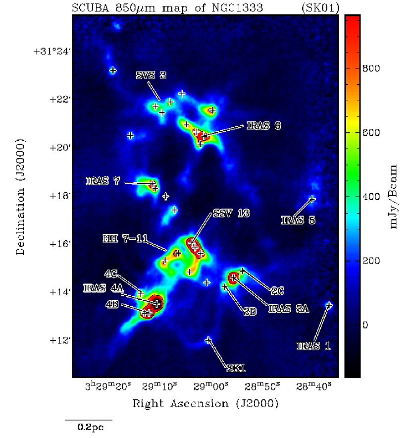
Figure 1: SCUBA 850$\mu$m dust continuum emission (SK01) in NGC 1333. Contours are 10, 20, 30, … 90% of the peak 6.68 Jy/beam. Plus symbols indicate the positions of SCUBA continuum sources identified by SK01.

NGC 1333 is a reflection nebula in Perseus which is associated with a molecular cloud, at a distance of 300 pc (de Zeeuw, Hoogerwerf & de Bruijne, 1999). It is also associated with two young star clusters identified in the near-infrared (Aspin, Sandell & Russell, 1994; Lada, Alves & Lada, 1996). Furthermore, it appears that a significant proportion of the stars seen in the near-infrared are pre-main sequence (Aspin, Sandell & Russell, 1994; Aspin, 2003). Figure 1 shows the 850 $\mu$m dust continuum emission towards NGC 1333, mapped by Sandell & Knee (2001; hereafter SK01). Plus symbols mark the positions of dust continuum peaks, established by SK01. The majority of the emission is found in the southern half of NGC 1333, which includes the IRAS 4 complex, the IRAS 2 complex and the SSV 13 complex. Each complex has previously been identified as a site of multiple star formation. NGC 1333 contains many well known outflows. Probably the best known is the outflow powered by SSV 13, or possibly the radio continuum source VLA 3 (Rodriguez et al., 1997). It is associated with the Herbig-Haro objects HH 7-11 to the SE and extends into the central cavity of NGC 1333 to the NW. In addition to this, there are outflows from both the IRAS 4 and 2 complexes, as well as IRAS 7 and 8 to the north.

SK01 note that the dust cores in NGC 1333 appear to have a mass function which is consistent with the stellar IMF. This has also been found for other regions of star formation such as in Ophiuchus (Motte et al., 1998; Johnstone et al., 2000) and IRAS 19410+2336 (Beuther & Schilke, 2004). Recent theories for star formation (eg. Bonnell et al. (2001a); Bate & Bonnell (2005)) indicate the stellar initial mass function is created at an advanced stage of evolution – during the accretion phase as matter is deposited onto the pre-main sequence star. Thus, the findings of stellar-like mass functions in prestellar cores is unexpected. One possible explanation is that the dust cores are transient phenomena and therefore are unlikely to be the sites of future generations of star formation. In order to decide whether such cores are transient or self-gravitating, it is necessary to observe cores in molecular line tracers so that kinematic information may tell us about their internal motions.

2 Observations and Data Reduction

2.1 BIMA Observations

Observations of NGC 1333 were made with the 10-element Berkeley Illinois Maryland Association (BIMA) interferometer, at Hat Creek, CA, USA, operating simultaneously at 89 GHz and 93 GHz. The maps were made by mosaicing together 126 pointings spaced by $\sim$1^′. With a $\sim$2′ FWHM primary beam at 3 mm, the resulting close-packed hexagonal pointing pattern provided full Nyquist sampling across the central 11′$\times$ 11′, yielding constant sensitivity across this field. The field was divided into 2 halves, with the southern half observed mostly in Fall 2001, and the northern half observed in Spring 2002. A total of 16 useable data tracks of 3-11 hours length were obtained over this period, in both the C- and D-array configurations. Both HCO⁺ (1–0) and N₂H⁺ (1–0) were observed in correlator windows of 256 channels each 0.16 km s^-1 wide. All 7 hyperfine components of N₂H⁺ (1–0) were observed in a single window. The remaining correlator windows were combined to provide 800 MHz bandwidth for simultaneous continuum observations.

We assume the line rest frequencies of 89.188253 GHz for HCO⁺(1–0) (Ulich & Haas, 1976) and 93.176258 GHz for the ‘isolated’ ($F_{1}F=01-12$) N₂H⁺(1–0) hyperfine component (Lee et al., 2001).

2.2 FCRAO Observations

Observations of NGC 1333 were made with the Five College Radio Astronomy Observatory (FCRAO) 14-m telescope on 2002 November 16. The data were taken in an On-The-Fly (OTF) mode using SEQUOIA, which is a MMIC multibeam receiver with a 32 pixel array, arranged as two 4$\times$4 arrays with orthogonal polarisations. Simultaneous observations were performed in N₂H⁺(1–0) and HCO⁺(1–0). The entire 11′$\times$ 11′ BIMA field was mapped with full Nyquist sampling. The FCRAO beam FWHM is about 50″ for these observations. Typical rms noise values are 0.048 K for HCO⁺ and 0.053K for N₂H⁺. Average system temperatures for HCO⁺ were 164 K and for N₂H⁺ were 174 K. The spectrometer is a digital autocorrelator with 1024 channels. Our spectral resolution was 25 kHz, corresponding to about 0.08 km s^-1. We assumed a conversion factor of 43.7 Jy/K.

2.3 Combination of Interferometer and Single Dish Data

The BIMA and FCRAO data were combined using the BIMA version of MIRIAD (Zhang, Q. private communication). The FCRAO data were initially demosaiced into single pointings corresponding to the BIMA pointings. Each pointing was then deconvolved with the FCRAO beam. UV points were randomly generated across the UV plane, with UV distances from 0 to uvmax, where uvmax corresponds to the size of the FCRAO dish (radius 7 m). The density of points in the UV plane was chosen such that they match the density of UV points from the BIMA data. The demosaiced, deconvolved FCRAO data were then transformed into the UV plane. Only data corresponding to the randomly generated UV points were recorded. The FCRAO and BIMA UV data were then combined, imaged and cleaned using standard MIRIAD reduction techniques.

The 1-$\sigma$ rms sensitivities of the cleaned data are 3 mJy beam^-1 for the continuum data, 330 mJy beam^-1 for both HCO⁺ and N₂H⁺. The final synthesized beam FWHMs were $\sim$10″($\sim$0.011 pc) for all data.

3 Results

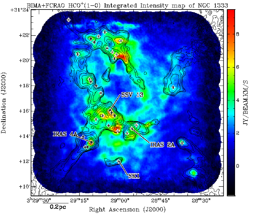
Figure 2: HCO⁺(1–0) integrated intensity map of NGC 1333. 0.2 Jy/beam km/s = 1$\sigma$. Contours are SCUBA 850$\mu$m emission (SK01). Contour levels are 0.02, 0.04, 0.08, 0.16, … 5.12 Jy/beam, where 0.02 Jy/beam = 1$\sigma$. Plus symbols indicate the positions of SCUBA continuum sources identified by SK01. HCO⁺ emission is seen to cover a larger area than submillimeter continuum, and loosely follows the submillimeter contours.

Figure 2 shows the HCO⁺(1–0) integrated intensity emission, compared to the 850$\mu$m continuum emission. Some general correspondence is seen between the two. For example, many of the peaks seen in the continuum map correspond to HCO⁺ peaks, including IRAS 4A, 4B, 2A, SSV 13. Also, some large scale structures show similar morphologies. On the other hand, some significant differences between the two are noticed: generally the HCO⁺ emission appears to cover a larger area than the continuum emission. Although the continuum map has been filtered spatially due to chopping during observations, this is probably because the HCO⁺ transition is more sensitive to lower column densities of material than the continuum observations. There are also differences in the distributions due to the effects of outflows which are discussed in §3.1.

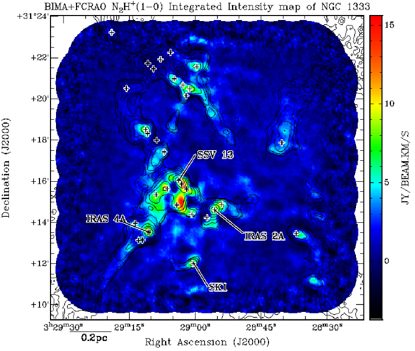
Figure 3: N₂H⁺(1–0) integrated intensity map of NGC 1333. 0.2 Jy/beam km/s = 1$\sigma$. Contours are SCUBA 850$\mu$m emission (SK01). Contour levels are 0.02, 0.04, 0.08, 0.16, … 5.12 Jy/beam, where 0.02 Jy/beam = 1$\sigma$. Plus symbols indicate the positions of SCUBA continuum sources identified by SK01. N₂H⁺ and submillimeter continuum closely follow each other in both extent and morphology. Small differences are seen between the two, however (eg. IRAS 2A/B/C).

Figure 3 shows the N₂H⁺(1–0) integrated intensity emission, compared to the dust continuum emission. The distribution of N₂H⁺ very closely follows that of the cold dust emission, much closer than that of the HCO⁺ emission. This similarity shows that N₂H⁺ is an excellent tracer of cold dust emission, as is known from studies of isolated cores (Tafalla et al., 2002). However, some small differences can be seen in Figure 3: the brightest spot in the dust continuum map is IRAS 4A, which is over twice as bright as anything else in the field of view. However, the brightest spot in the N₂H⁺ map is located an arcminute to the south of SSV 13. The IRAS 2 complex includes three dust continuum peaks 2B, 2A and 2C running from SE to NW, respectively. Whilst IRAS 2A is clearly the brightest in both continuum and N₂H⁺ integrated intensity emission, IRAS 2C is a very weak continuum source but is almost as bright in N₂H⁺ emission as IRAS 2A. Furthermore, IRAS 2B has stronger emission in continuum than IRAS 2C, but appears almost devoid of any N₂H⁺ emission. Jørgensen et al. (2004a) have investigated the chemistry of N₂H⁺ in this region and conclude that the apparent differences are due to varying degrees of thermal processing: 2B is the warmest and oldest source, having destroyed N₂H⁺ around it, IRAS 2C is the youngest and coolest source with physical conditions that favor the production of N₂H⁺, and IRAS 2A has a temperature and age somewhere between the two. One other major difference between the continuum and N₂H⁺ morphologies is that near SVS 3 (to the NE of the field of view), there is a large region which clearly shows continuum emission consisting of at least five sources identified by SK01, spanning an area approximately 0.3′$\times$0.2′, but shows no evidence of N₂H⁺ emission.

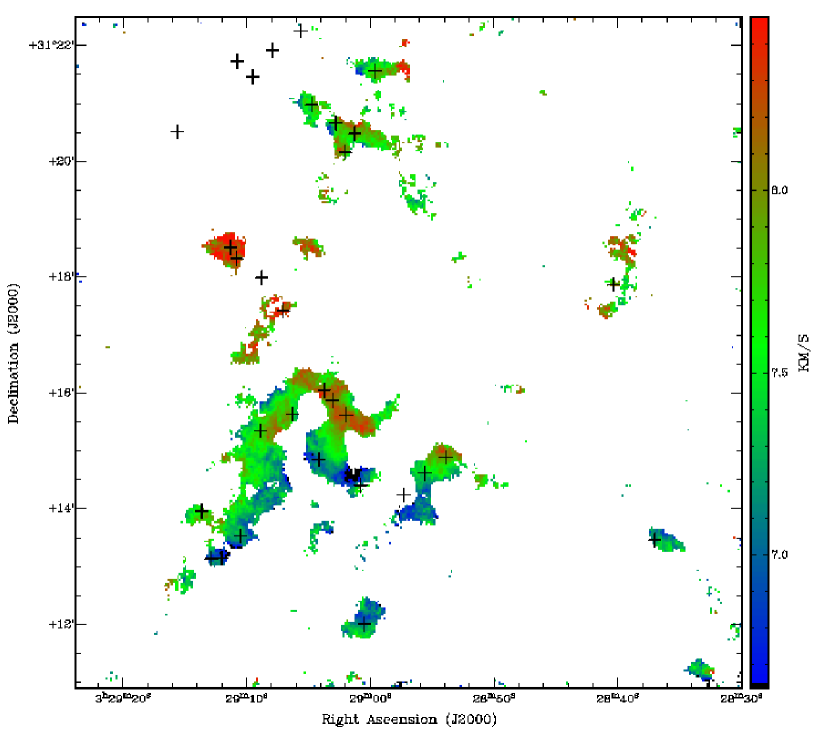
Figure 4: N₂H⁺ first moment map of NGC 1333, showing the line of sight motions of the gas. Plus symbols indicate the positions of SCUBA continuum sources identified by SK01.

Figure 4 shows the first moment map of line of sight velocities for N₂H⁺. Most of the emission is found between velocities of 6.5 and 8.5 km s^-1. Overall, the emission in the southern part of NGC 1333 (south of 31^∘ 14^′) appears blueshifted with respect to emission in other parts of the region. N₂H⁺ emission close to IRAS 7 appears to be redshifted from the bulk of the emission. Previously, Ho & Barrett (1980) suggested that bulk motions traced by ammonia were indicative of rotation. However, it appears their data were strongly biased by the redshifted emission associated with IRAS 7. If NGC 1333 were undergoing rotation, then we would expect to see redshifted emission over a much larger area, rather than being confined around IRAS 7. We still see a large area to the south with blueshifted emission, but apart from IRAS 7, the rest of the gas appears to be moving at approximately the same velocity. Therefore, the gas traced by N₂H⁺ does not show significant signs of large-scale rotation, although there are clear differences between motions on smaller scales.

3.1 HCO⁺ outflows

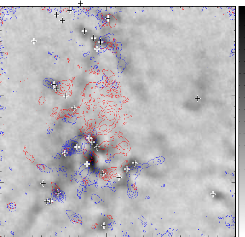
Figure 5: HCO⁺ outflows in NGC 1333. The greyscale is N₂H⁺ integrated intensity. Blue contours represent HCO⁺ integrated emission from -5.5 to +5.3 ${\rm km}\,{\rm s}^{-1}$. Red contours represent HCO⁺ integrated emission from 10.4 to 16.4 ${\rm km}\,{\rm s}^{-1}$. The lowest contour (both red and blue) is at 9 Jy/beam and increase in steps of 4 Jy/beam to a maximum of 33 Jy/beam for the red and 41 Jy/beam for the blue.

Knee & Sandell (2000) have previously described these outflows in detail, however we include Figure 5 which shows the blue and red lobes of outflows in the HCO⁺ map which shows the outflows at higher resolution than the maps of Knee & Sandell (2000). The blue-shifted lobe from SSV 13 (or VLA 3) is clearly the brightest emission in the field of view.

Apart from the previously detected outflows, we note that the large, redshifted lobe of emission in the center of the field of view coincides with the central cavity (Knee & Sandell, 2000). The central cavity is filled with high velocity gas from outflows and Knee & Sandell (2000) suggest it was created by these outflows. Furthermore, the red lobe coincident with the central cavity appears to be bounded by the filamentary structure of dense gas traced by N₂H⁺. We therefore conclude that the outflow(s) responsible for this redshifted lobe fill the cavity with high velocity gas. It is clear that the bulk of this lobe comes from the outflow associated with either SSV 13 or VLA 3, but the north–south outflow from IRAS 2A also projects into this area, as well as the outflow from IRAS 7. It is even possible that there is a red-shifted outflow lobe from SSV 13B, located to the west of SSV 13 that also projects into the cavity. These overlapping outflows make interpretation of the red-shifted emission in this region difficult.

4 Discussion

4.1 Analysis of N₂H⁺ cores

As previously mentioned, the N₂H⁺ map very closely follows that of the dust continuum emission. Therefore we can analyse the density structure of NGC 1333 by observing the emission in this transition. Because N₂H⁺ is a spectral line, we can also use the velocity information to help discriminate cores along the same line of sight. The N₂H⁺ (1–0) transition has seven hyperfine components which could potentially be used for better velocity determination of the cores, however, because most of these hyperfine components are blended, we choose to restrict our analysis to the isolated hyperfine component. This has the unfortunate effect of reducing our overall signal from this transition.

Clumpfind (Williams et al., 1994) is an algorithm for identifying peaks of emission in a data cube. It was originally used to identify clumps in single dish spectra. It works in a way similar to contouring a map: where it finds closed contours a core is identified. The algorithm also extends the size of the core by including adjoining pixels down to a detection threshold. If a core is extended until it runs into another core (with its own separate peak), the algorithm stops extending the core on that front. The outcome is an interconnected cube of identified cores that appear similar to what would be expected if one identified cores and core boundaries by eye. Thus, all the real emission above the detection threshold is categorised as material belonging to some core.

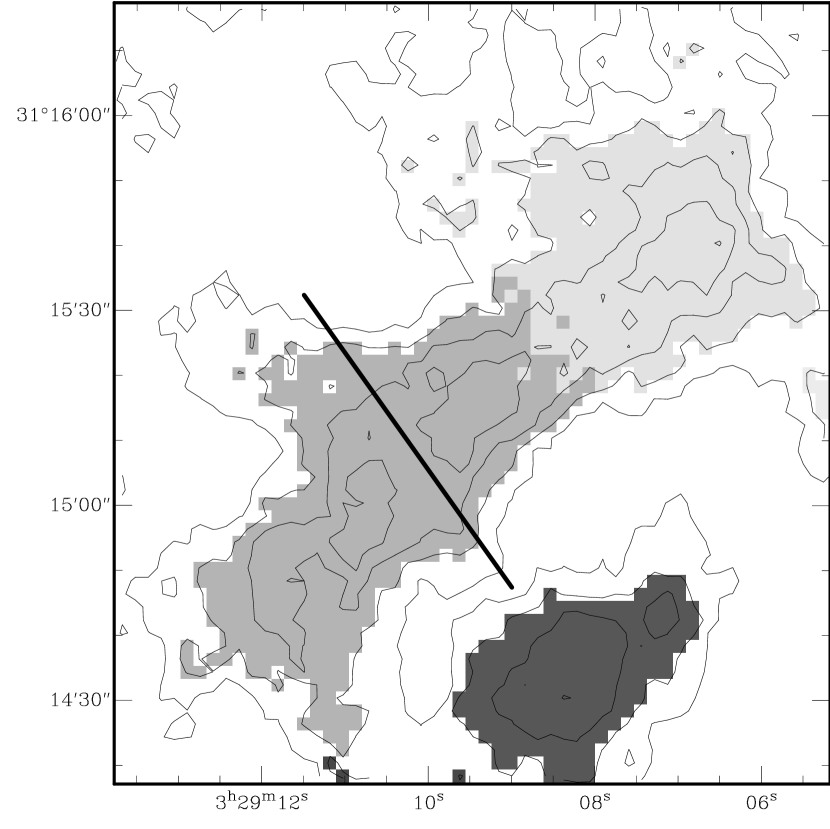
Figure 6: Clumpfind results for a small portion of the N₂H⁺ data cube. The different shadings represent the identified cores. The contours are N₂H⁺ emission at the same levels as those used by clumpfind: 0.244, 0.488, 0.732… 2.196 Jy/beam. The diagonal line represents an artificial break in the largest core that should be applied to separate this core into two individual cores.

We chose to identify cores using the default setting of searching down to twice the rms noise level, with spacing between contours also twice the rms noise (0.244 Jy/beam). We require that each core must contain at least enough pixels to fill one beam. We found that sometimes clumpfind was inadequate for separating out multiple cores. For example, Figure 6 shows a small portion of one velocity channel of the N₂H⁺ data cube, with identified cores shaded differently. The contours are the N₂H⁺ emission and coincide with the contours used by clumpfind to identify cores. Three cores are identified by clumpfind in this region. However, clumpfind failed to break up the largest core along the line shown. We believe that cores like this should be divided because there are closed contours on both sides of the dividing line. In this case, we divide the core into two by running clumpfind again with a smaller separation of contours. In this manner, we have avoided limitations of the clumpfind program and we believe we have separated cores in an unbiased manner. Note that whilst the smallest identified clump, to the south with the darkest shading, appears to show two closed contours, the smaller peak contains less than the required number of pixels to fill a beam. Therefore, it is not assigned to be a separate core.

Many of the weakest cores identified by clumpfind were found to be noise spikes. We therefore employed a reality check on all clumps. Because we have data on all seven hyperfine components of the N₂H⁺ line, we checked the N₂H⁺ spectrum of the core to make sure all seven components were visible. This is a very robust test because we identified our cores on a weak hyperfine component and so it was easy to discern a noise spike from a true N₂H⁺ core. Furthermore, we checked that the morphology of the core identified in the isolated hyperfine component was similar to that seen in the brighter hyperfine components. As a result we have identified 93 cores.

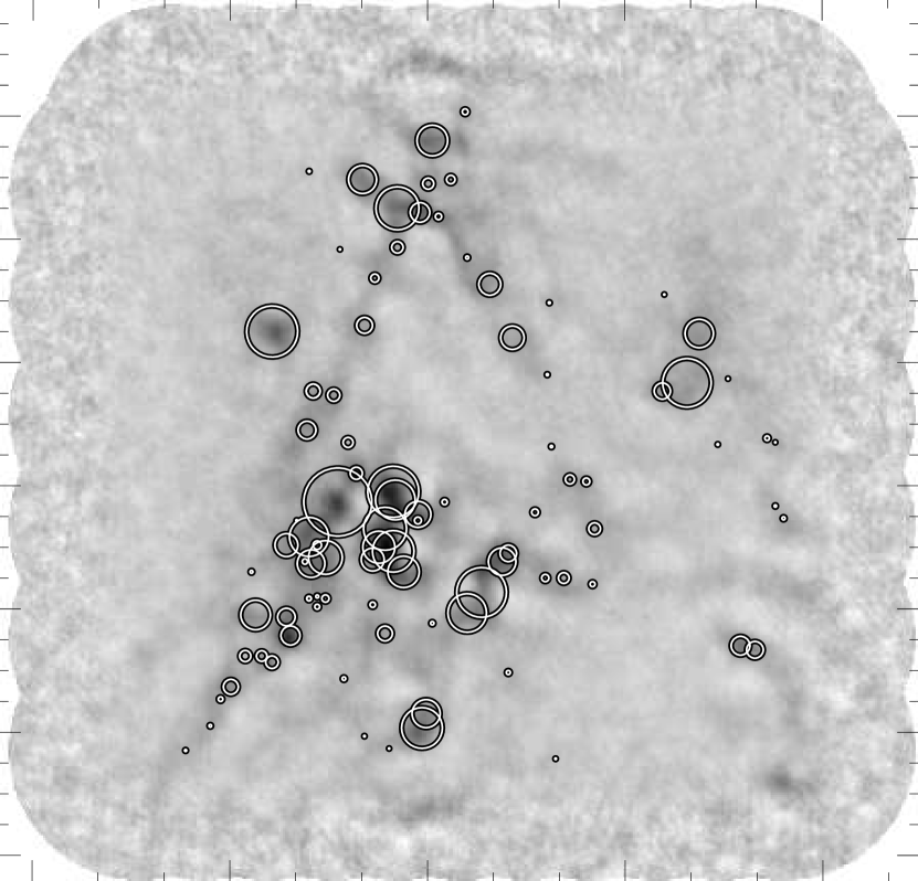
Figure 7: Distribution of identified N₂H⁺ cores. The greyscale is the N₂H⁺ integrated intensity map. Numbers on the left correspond to the positions of cores listed in Table 1. The radius of the rings on the right is proportional to the ${\rm M}_{\rm LTE}$ for each core, listed in Table 1. Note: weak cores are seen on the edges of the map, which were not identified by clumpfind as they lie outside the fully sampled region of the BIMA observations. An example is located at 03 28 33.0 +31 11 12.

The details of the cores are shown in Table 1 and their relative positions are shown in Figure 7. As mentioned previously, there are five dust continuum cores to the NE (SK01) that do not exhibit any N₂H⁺ emission. Apart from these, nearly every SK01 continuum core coincides with an N₂H⁺ core. The only exception is core 17 from SK01, located to the SW of IRAS 6, which also does not show any N₂H⁺ emission. Figure 8 shows example N₂H⁺ and HCO⁺ spectra for two cores (27 and 85), which are examples of high and low mass cores, respectively. It is clear that the N₂H⁺ emission towards core 85 (the lower mass core) is well detected. As can be seen in Figure 7, many of the cores are found in filamentary structures of high aspect ratio. These filaments are seen extending to the SE and SW of IRAS 6 and to the SE of SSV 13, through IRAS,4. The filaments appear to closely (but not exactly) follow the dust distribution (SK01). We also calculate the core mass by two different methods: the LTE approximation and by using the virial theorem. These are discussed in detail in the following sections.

4.1.1 LTE Mass

We assume that the column density traced by the N₂H⁺ (1–0) transition in a core is given by (Williams et al., 1994)

$${\rm N}=\frac{3\epsilon_{0}\,{\rm k}}{\pi^{2}\nu\mu^{2}}\left(1-{\rm e}^{\frac{-{\rm h}\nu}{\rm kT}}\right)^{-1}\left(\frac{{\rm T}}{({\rm J}[{\rm T}]-{\rm J}[2.73])}\right)\int{\rm T}({\rm v})\;{\rm dv}$$ (1)

where

$${\rm J}[{\rm T}]=\frac{{\rm h}\nu}{{\rm k}\left({\rm e}^{\frac{{\rm h}\nu}{{\rm k}{\rm T}}}-1\right)}$$ (2)

where $\epsilon_{0}$ is the permittivity of free space; $\mu$ is the dipole moment for N₂H⁺ (1–0), which is 3.4 Debye ($1.13\times 10^{-29}$ C m) and $\int{\rm T}({\rm v})\;{\rm dv}$ is the line integrated intensity. We assume the temperature of the gas (T) to be 15 K. We choose 15 K because it is on the upper limits for temperatures of isolated cores (Benson & Myers, 1989) and we expect temperatures to be slightly higher in clustered regions. However, we caution that uncertainties in temperature may lead to an error as large as a factor of a few. To convert this to a hydrogen column density, we assume the relative abundance of N₂H⁺ is $1.8\times 10^{-10}$. We find values quoted in the literature from $3\times 10^{-11}$ (Bergin et al., 2002) for the isolated core B68 to $5\times 10^{-9}$ for IRAS 2 in NGC 1333 (Jørgensen et al., 2004a), which both appear to be extreme cases. Reasons for assuming this abundance are given in §4.1.3, but we note here that our assumed relative abundance lies within the extremes and will be a representative value for most cases, although we might expect deviations of up to an order of magnitude in extreme situations. Thus, the hydrogen column density is given by:

$${\rm N}_{\rm H}=9\times\frac{\rm N}{1.8\times 10^{-10}}$$ (3)

The factor of 9.0 in the above equation is determined by measuring the average ratio of the flux of the isolated N₂H⁺ hyperfine component to the total flux, and assumes the line is optically thin. The LTE mass is then calculated using:

$$\left(\frac{{\rm M}_{\rm LTE}}{{\rm M}_{\odot}}\right)=3.756\times 10^{-32}\;\overline{m}\;\left(\frac{{\rm N}_{{\rm H}_{2}}}{{\rm m}^{-2}}\right)\left(\frac{{\rm T}_{\rm av}}{\rm K}\right)\;\left(\frac{\rm d}{\rm pc}\right)^{2}\;\left(\frac{\rm pixsize}{\rm arcsec}\right)^{2}\;\left(\frac{\Delta{\rm V}}{{\rm km}\,{\rm s}^{-1}}\right)\;{\rm N}_{{\rm PIX}}$$ (4)

where $\overline{\rm m}$ is the mean molecular weight of the gas, taken to be 2.3; ${\rm N}_{{\rm H}_{2}}$ is taken from Equation 3 above and assumes the gas is molecular; ${\rm T}_{\rm av}$ is the mean brightness temperature of each pixel of the core identified by clumpfind; d is the distance to NGC 1333, which is taken to be 300 pc (de Zeeuw, Hoogerwerf & de Bruijne, 1999; Belikov et al., 2002); pixsize is the size of the data cube pixels in arcseconds, which is 2″ for our data; $\Delta{\rm V}$ is the velocity width of each channel, $0.157\,{\rm km}\,{\rm s}^{-1}$; ${\rm N}_{\rm PIX}$ is the number of pixels that are identified with the core.

The uncertainty in the calibration of our flux density scale will contribute an error to the derived LTE masses. We estimate this error to be no greater than 20%. Our assumed distance of 300 pc comes from HIPPARCOS measurements, however we note distances in the literature ranging from 220 (SK01) to 350 pc (Di Francesco et al., 2001). Thus masses and sizes will need adjusting when comparing to work using different distances. We also anticipate that uncertainty in the temperature of the gas (we assume 15 K) will also contribute an error which may be as large as a factor of a few. We believe the error associated with the uncertainty in the relative abundance of N₂H⁺ to be the largest error in the LTE mass calculation.

4.1.2 Virial Mass

We can also use the N₂H⁺ data to calculate virial masses for the cores using:

$${\rm M}_{\rm VIR}=210\times\delta{\rm V}^{2}\;{\rm r}$$ (5)

where $\delta{\rm V}$ is the line FWHM and r is the effective radius of the core (column 5 of Table 1)(Caselli et al., 2002). Equation 5 assumes a uniform density profile. If we assume a density profile that falls off as ${\rm r}^{-2}$, then the constant 210 in Equation 5 changes to 126 (Williams et al., 1994). Thus, our calculation of the virial mass of the cores may decrease by a factor of two. We also note that the virial mass ignores magnetic fields, as well as the effects of an external pressure, which may have a significant effect on the virial mass in a region such as NGC 1333, due to mechanical pressure from outflows impinging on the cores. Furthermore, outflows are likely to be hot, which also may increase the pressure on the cores.

4.1.3 Comparison of ${\rm M}_{\rm LTE}$ and ${\rm M}_{\rm VIR}$

The LTE mass is a measure of the amount of matter located within a core, whereas the virial mass is a measure of amount of matter required to keep a core bound. Therefore, we can compare the two masses to evaluate whether a core has enough self gravity to stay bound or not. If a core is bound, then the LTE mass should be greater than, or equal to, the virial mass. The distribution of virial masses with respect to LTE masses for the same core is shown in Figure 9. We have chosen a value of the N₂H⁺ relative abundance ($1.8\times 10^{-10}$) such that the points in Figure 9 are distributed evenly about the line of equality (${\rm M}_{\rm LTE}={\rm M}_{\rm VIR}$), shown by the solid line. If we assume a different relative abundance then this will have the effect of sliding the diagonal line of equality along the horizontal axis in Figure 9. Because of the uncertainty in the abundance, we cannot be sure whether individual cores are bound or unbound based solely on a comparison of their LTE and virial masses.

M_VIR and M_LTE are correlated with a correlation coefficient of 0.88 over a range in M_LTE of $\sim$40, despite the individual uncertainties in M_VIR and M_LTE. Such a correlation is unlikely to be a coincidence, suggesting that most of the cores are self-gravitating, at both high and low ends of the mass range. If proportionately more of the lowest mass cores were unbound, compared to the highest mass cores, then we would expect to see the distribution of points in Figure 9 to turn up towards the virial mass axis, in the lower left (lowest mass) corner. However, there are approximately equal numbers of points above (19) and below (18) the solid line with ${\rm M}_{\rm LTE}<0.3$, as compared to approximately equal numbers of points above (29) and below (27) the solid line with ${\rm M}_{\rm LTE}>0.3$. The curved line in Figure 9 is a second order polynomial fit to the data points, given in Equation 6:

$${\rm Log}({\rm M}_{\rm VIR})=0.071+1.38\,{\rm Log}({\rm M}_{\rm LTE})+0.26\,({\rm Log}({\rm M}_{\rm LTE}))^{2}$$ (6)

Whilst the polynomial fit in Figure 9 does show a small turn up at the lower mass end, the turn up is small compared to the scatter in the data points. Therefore we do not consider it significant. Thus, we have no evidence for such a turning up of the distribution in our data. We conclude that many of the lower mass cores are likely to be self-gravitating, and are not transient objects.

Some of the higher mass cores can be expected to be bound, since they are associated with protostars, such as core 37 (IRAS 4A), core 38 (IRAS 4B), core 36 (IRAS 2C) and core 15 (IRAS 7). Below we detail some of the properties of these cores.

Core 37 (IRAS 4A). We calculate an LTE mass of $0.7\,{\rm M}_{\odot}$ and a virial mass of $1.0\,{\rm M}_{\odot}$. This might suggest that the core is unbound, but we know this is not the case because IRAS 4A contains at least two protostars (Lay, Carlstrom & Hills, 1995): an alternate explanation is needed. IRAS 4A was observed by Di Francesco et al. (2001) in N₂H⁺ at a higher resolution than our observations. They calculate the LTE mass of IRAS 4A to be $0.73{\rm M}_{\odot}$, assuming the distance to NGC 1333 is 350 pc and X(N₂H⁺) = $6.0\times 10^{-11}$. Converting this mass using our preferred distance (300 pc) and N₂H⁺ relative abundance ($1.8\times 10^{-10}$), this is equivalent to $0.18{\rm M}_{\odot}$, a factor of 4 lower than our derived value. This is partly because their higher resolution observations filtered out some of the extended emission. By combining the BIMA data with the FCRAO data, we have minimised this problem. The relative abundance of N₂H⁺ makes a significant difference to the derived LTE mass. We can check our derived relative abundance by comparing LTE mass to that derived from dust continuum measurements by SK01. SK01 determine the mass of IRAS 4A to be 1.5 ${\rm M}_{\odot}$, assuming a distance of 220 pc. To reproduce our LTE mass, we require a relative abundance of $5\times 10^{-11}$, similar to that derived by Di Francesco et al. (2001). Therefore, we agree with the finding of Di Francesco et al. (2001) that there is an unusually low relative abundance of N₂H⁺ at IRAS 4A. We see the effect of this lowered abundance when comparing the relative intensities of N₂H⁺ and 850$\mu$m continuum emission at IRAS 4A in Figure 3. The continuum contours strongly peak at the position of IRAS 4A whilst the N₂H⁺ emission is only a weak peak at this position.

A possible explanation for the low abundance is that IRAS 4A is the source of an outflow, which is traced by HCO⁺. The HCO⁺, and CO, will be enhanced in the gas phase by the shocks from the outflow. Since both HCO⁺ and CO destroy N₂H⁺ (Jørgensen et al., 2004b), we expect to find a lower N₂H⁺ abundance here. An alternate explanation is that IRAS 4A has undergone thermal processing of its N₂H⁺, thereby reducing the N₂H⁺ abundance.

Core 38 (IRAS 4B). We calculate an LTE mass of 0.5 ${\rm M}_{\odot}$ and a virial mass of $1.4\,{\rm M}_{\odot}$. Again, this might imply the core is unbound, but we know this is not the case (Lay, Carlstrom & Hills, 1995). Di Francesco et al. (2001) have also observed this core at higher resolution and find an LTE mass of 0.41 ${\rm M}_{\odot}$, using the same assumptions as for IRAS 4A. Here, we assume that again there is a significant amount (a factor of 5) of missing N₂H⁺ flux in the data of Di Francesco et al. (2001). Comparing our LTE calculations to the dust continuum mass derived by SK01, we can estimate the relative N₂H⁺ abundance. SK01 derive a combined mass of 0.63 ${\rm M}_{\odot}$ for IRAS 4B west and east. We combine the masses for the west and east components here because our resolution was not sufficiently high enough for clumpfind to separate N₂H⁺ emission surrounding the two protostars. The N₂H⁺ abundance is then estimated to be $1\times 10^{-10}$, close to assumed abundance of $1.8\times 10^{-10}$.

Core 36 (IRAS 2C). We calculate an LTE mass of 0.6 ${\rm M}_{\odot}$ and a virial mass of 0.4 ${\rm M}_{\odot}$. IRAS 2C has been identified as one of the youngest sources in NGC 1333 and is most likely a Class 0 source (SK01). SK01 also use their dust continuum observations to derive a mass of 0.05 ${\rm M}_{\odot}$. In this case, it appears there is an N₂H⁺ abundance enhancement of about 6 over the assumed average value.

Core 15 (IRAS 7). We calculate an LTE mass of 2 ${\rm M}_{\odot}$ and a virial mass of 1.6 ${\rm M}_{\odot}$. SK01 calculate a mass of 0.16 ${\rm M}_{\odot}$ for the combined contributions of SM 1 and SM 2. Again, it appears the abundance may be enhanced by a factor of a few over the average value.

4.2 Association of cores with stellar sources

Recent observations of NGC 1333 with the Spitzer Space Telescope (Gutermuth et al., 2006) allow us to compare the incidence of our N₂H⁺ cores with infrared stars. All the stars we correlate with N₂H⁺ cores are known to be pre-main sequence stars within NGC 1333, by nature of their infrared colors, using the bands at 3.6, 4.5 and 5.8$\mu$m, which identifies Class I, II and III sources. In addition to this, we used 24 and 70$\mu$m Spitzer images to associate cores with Class 0 sources. We note that all previously known Class 0 sources in the field of view are easily detected at these longer wavelengths. The infrared observations have a sensitivity limit of around 0.05 ${\rm M}_{\odot}$, which is similar to the mass limit of our detected cores. We consider a star associated with an N₂H⁺ core if any part of the N₂H⁺ core, as defined by clumpfind, overlaps with the peak of the infrared emission.

Using the same association critera, we have used a monte carlo simulation to test how many chance alignments of N₂H⁺ cores and infrared sources we might expect. To do this, we assume an average N₂H⁺ core size of 0.015 pc and randomly place 93 simulated cores in the field of view and count the number of chance alignments. This process is repeated to derive a distribution of expected chance alignments. From these simulations, we expect 3.5 chance alignments of N₂H⁺ cores with infrared stars. This low number of chance alignments is unlikely to affect our results discussed below.

N₂H⁺ cores with associated stars are shown in Figure 9. It is clear from this figure that N₂H⁺ cores associated with stars tend to have higher masses than those without. This can also be seen in Figure 10, as well as the distributions of other attributes of the N₂H⁺ cores. Both the distributions of N₂H⁺ core LTE and virial masses are extremely unlikely to come from the same population. Figure 10 also shows that cores without associated stars are generally smaller than those with stars. Implications of this are discussed further in §4.3.

The N₂H⁺ core line FWHM is generally smaller for cores not associated with stars. This is what would be expected if the stars are active in creating local turbulence through their stellar winds and outflows. Such winds and outflows should stir up the immediate environment of surrounding gas, increasing the measured line FWHM. The tendency of cores with associated stars to have larger line widths has been seen in ammonia cores (Benson & Myers, 1989; Jijina, Myers & Adams, 1999).

4.3 Mass distribution of the cores

Recent simulations by Bonnell et al. (2001a) and Bate & Bonnell (2005) indicate that the initial mass function (IMF) is created at an advanced stage of evolution. Initially all cores start with the same mass, which is determined by the opacity limit for fragmentation. Stars build up their mass through accretion. The final mass of the star is then determined by stochastic ejection of the stars from the cluster due to dynamical interactions. However, previous observations of pre-stellar dust cores in the rho Ophiuchi main cloud (Motte et al., 1998; Johnstone et al., 2000) show that the mass distribution of some of the pre-stellar cores resembles the IMF. This suggests that the IMF may be locked in at the pre-stellar stage, in contradiction to the simulations. The previous observations by Motte et al. (1998) and Johnstone et al. (2000) were continuum measurements and so no linewidth information for the cores is known. It is therefore possible that the pre-stellar cores are transient phenomena and may not form stars, as suggested by Ballesteros-Paredes & Mac Low (2002). Our N₂H⁺ data have shown that in NGC 1333 at least, the N₂H⁺ cores appear to be close to virialised and therefore a significant proportion are likely to be bound and are therefore more likely to form stars.

In Figure 11, we show the distribution of core LTE and virial masses. The LTE and virial mass distributions are very similar. Furthermore, we find these distributions similar to the average field star IMF, although the LTE and virial mass distributions do not show a decrease for lower mass cores, as is seen in the IMF. Such similarities between the stellar IMF and the the mass function of dust cores has also been found by Motte et al. (1998), Johnstone et al. (2000) and Stanke et al. (2006), who suggested this is evidence that the IMF may be locked in at this early stage of star formation. A problem with comparing the mass function of dust cores and stars is that it is not clear whether the dust cores are bound or not – no information on their internal motions is known. The N₂H⁺ data allow us to overcome this problem. If the N₂H⁺ cores are bound regardless of mass, this suggests that such emission does not trace transient structures formed out of turbulent fluctuations. Therefore, this implies the entire mass distribution consists of objects that may potentially form stars.

It is interesting to note that in Figure 10, we see a flat distribution of core masses (both LTE and Virial) for those cores associated with stars. This flat distribution is clearly unlike the field star IMF. There appear to be too few low mass cores to form a mass function similar to the field star IMF. Because both the N₂H⁺ and infrared observations have a sensitivity limit of around 0.05 ${\rm M}_{\odot}$, we do not believe this is an effect of the sensitivity limits.

As a core forms a star, it loses gas mass. If lower mass cores lose a bigger proportion of their mass than do higher mass cores, the lower mass cores move left in the distribution shown in Figure 10 more than the higher mass cores, making the mass function distribution shallower. But if more of the high mass cores make multiple stars than do low mass cores, the mass function should look steeper. These are two competing effects that may well affect the distribution we see. Future research should be undertaken to identify the cause of this apparent flattening of the mass function.

4.4 Clustering

NGC 1333 is known as a region of clustered star formation (Aspin, Sandell & Russell, 1994; Lada, Alves & Lada, 1996). As can be seen from Figure 7, the N₂H⁺ cores also appear to cluster, showing a concentration in the IRAS 4/IRAS 2/SSV 13 region, with a particular concentration of cores around SSV 13. In Figure 12, we show a comparison of clustering properties of N₂H⁺ cores for varying LTE masses. For each core, the upper plot shows the number of cores that are within a radius of 0.2 pc, whilst the lower plot shows how far away the nearest core is. Both distributions are a measure of the clustering properties of the cores throughout their mass spectrum. As can be seen, there is no clear correlation between either of the distributions. However, it appears that only a small proportion of cores with M$<0.2$ M_⊙ have more than four neighbours (43%), whereas proportionately more of the higher mass cores have more than four neighbours(79%), But this trend is weak and does not appear for other choices mass cutoff. This implies that there is little significant increase in the likelihood of finding a more massive core in a clustered region, than a lower mass core. Furthermore, when cores are separated into those that are associated with stars (filled in circles) and those that are not (open circles), there is no significant difference between the two populations.

4.5 Motions of the cores

An important difference between isolated and clustered star formation is the effects of turbulence, which are expected to be larger in the clustered environment. Di Francesco, André & Myers (2004) have studied the relative motions of cores in the Ophiuchus A cluster region. The Oph A observations have a higher spatial resolution ($10\arcsec\times 6\arcsec$, corresponding to $1250\times 750$ AU) than the NGC 1333 observations ($10\arcsec\times 10\arcsec$, corresponding to 3000 AU) but cover a smaller area ($\sim$0.1 pc for Oph A and $\sim$1.0 pc for NGC 1333). Di Francesco et al. (2004) found little dispersion between the line-of-sight velocities of the cores they detected within Oph A with an rms dispersion of only 0.17 km s^-1. For NGC 1333, we find a mean line-of-sight velocity of 7.66 km s^-1 and an rms dispersion of 0.46 km s^-1. This is larger than that found for Oph A. Examination of the N₂H⁺ data cube suggests that this is because there appear to be two regions of N₂H⁺ emission along the same line of sight in the vicinity of SSV 13. These are traced by cores 4, 5, 6, 7, 16 and 84 which all have velocities greater than 8.1 km s^-1, and cores 1, 2, 3, 17, 18, 52 and 55 which all have velocities less than 7.8 km s^-1. For each velocity component, we find the rms dispersion is 0.14 and 0.34 km s^-1 for cores greater than 8.1 and less than 7.8 km s^-1, respectively. Thus, it appears the velocity dispersion is larger in NGC 1333 than in Oph A, even taking into account the multiple velocity components along the line of sight in NGC 1333. For the N₂H⁺ core line widths, we find an average value of 0.38 km s^-1 and an rms dispersion of 0.14 km s^-1. These numbers are very similar to those found by Di Francesco et al. (2004) in Oph A: 0.39 km s^-1 and 0.11 km s^-1, respectively. So it appears that individual core kinematic properties are similar in Oph A and NGC 1333, but there are larger relative motions of the cores in NGC 1333. However, this may be an effect for measuring a much larger area in NGC 1333. In order to compare the two clusters in more detail, more cores need to be identified on a similar size scale to the Oph A observations.

We can investigate the motions of cores within the filamentary structures to the SE of SSE 13 and to the SW and SE of IRAS 6. If we assume that the filamentary structures are true filaments; ie. that they will also appear as filaments when observed orthogonal to the current viewing angle, then we can estimate how long it will take for cores to move the length of a filament, based on the observed velocity dispersion. This will tell us the typical timescale we might expect the filaments to survive. We find velocity dispersions of cores within the filament to the SE of SSV 13 (0.6 pc long), and to the SW (0.5 pc long) and SE (0.5 pc long) of IRAS 6 to be 0.23, 0.27 and 0.24 km s^-1, respectively. Taking an average of 0.25 km s^-1, and assuming cores must travel 0.5 pc for a filament to dissipate, we calculate the filaments may survive for $2\times 10^{6}$ years. Such a long time implies these filaments may well be stable features.

Previously, Walsh, Myers & Burton (2005) have investigated the relative motion of star forming cores with respect to their surrounding envelopes. This was done by observing N₂H⁺(1–0) which traces the high density core motions and ¹³CO (1–0) and C¹⁸O (1–0) which trace the low density surroundings. They found little evidence for any ballistic relative motions. This is in contradiction to previous theoretical work (Bonnell et al., 1997, 2001b) which suggested that a star’s final mass was determined by its motion through its natal cloud. The observations of Walsh et al. (2005) were focused mainly towards regions of isolated star formation, with a very small number of regions close to clustered environments. Their results were clear for the case of the isolated regions of star formation, but inconclusive for the clustered regions. With these new data, we are able to look for relative motions in NGC 1333 and thus extend the work to include a clustered region of star formation.

We use the line center velocities of the N₂H⁺ cores given in Table 1 as our high density tracer and the ¹³CO (1–0) and C¹⁸O (1–0) FCRAO maps of Ridge et al. (2003) covering NGC 1333 as the low density tracers. We determine the difference in line center velocities by using the N₂H⁺ core velocities given in Table 1 and fitting a gaussian to the ¹³CO and C¹⁸O line profiles of the spectrum that coincides with the peak of the N₂H⁺ core. Not all N₂H⁺ cores could be included in the analysis. This is because some of the CO spectra were too confused to reliably determine a relevant line center velocity. Figure 13 shows the difference in the line center velocities, which can be compared to Figure 1 of Walsh et al. (2005) for the case of isolated cores.

The top of Figure 13 shows simulated line profiles for the average line width of N₂H⁺, ¹³CO and C¹⁸O. As was previously discussed by Walsh et al. (2005), if we expect there to be no motions of the high density cores with respect to their surroundings, then we would expect to see line center velocity differences distributed like the line profile for the N₂H⁺ transition. If there are significant motions of the core, then we would expect to see broader distributions resembling the CO line profiles. Figure 13 shows that line center velocity differences have a distribution somewhere between these two extremes: The rms difference between N₂H⁺ and ¹³CO is 0.57 km s^-1 and between N₂H⁺ and C¹⁸O is 0.53 km s^-1. These numbers can be compared to the average ¹³CO FWHM of 1.18 km s^-1, average C¹⁸O FWHM of 1.00 km s^-1 and average N₂H⁺ FWHM of 0.38 km s^-1. Unfortunately, our results may suffer from some errors that were avoided by Walsh et al. (2005). This is because we are using different telescopes, and observations were made under different conditions. One of the greatest source of errors is that our BIMA N₂H⁺ data are of much higher spatial resolution than the FCRAO CO data. Thus it is likely that the CO data trace somewhat different columns, compared to the N₂H⁺ data. This will give an apparent increase in the differences of measured line center velocities between N₂H⁺ and the CO isotopes. This has the effect of rendering our results uncertain as to whether we can tell if there are relative motions of the cores, although we note that it seems to be consistent with the cores not moving ballistically. In order to obtain a clear answer, it will be necessary to obtain CO data with the same resolution as the N₂H⁺ data, which is beyond the scope of this work.

5 Summary and Conclusions

We have used both the BIMA and FCRAO radiotelescopes to observe HCO⁺ (1–0) and N₂H⁺ (1–0) in the clustered star forming region NGC 1333. Comparison with submm continuum images shows that the N₂H⁺ emission very closely follows the dust continuum, showing it is an excellent tracer of quiescent gas. HCO⁺, on the other hand, shows overall similarities with dust continuum, but appears more extended and also traces outflowing gas.

We have identified 93 N₂H⁺ cores in the field of view, with masses between approximately 0.05 ${\rm M}_{\odot}$ and 2.5 ${\rm M}_{\odot}$. Whilst uncertainties in the relative abundance of N₂H⁺ do not allow us to conclude whether or not individual cores are bound, the trend of core properties suggests that most will be bound. Furthermore, there is no up-turn of the distribution of core Virial-LTE masses, which would suggest that the lowest mass cores are not bound and therefore transient phenomena. Our conclusion is that even these low mass cores are likely to remain bound and eventually form stars, or brown dwarfs. If the N₂H⁺ cores are bound regardless of mass, this suggests that such emission does not trace transient structures formed out of turbulent fluctuations. Therefore, this implies the entire mass distribution consists of objects that can potentially form stars.

The mass function of the N₂H⁺ cores is consistent with the field star IMF, suggesting that the distribution of masses may be locked in at the pre-stellar phase, in contradiction to theories of mass accumulation by competitive accretion. We find that the mass function of core associated with stars is flat, and unlike the IMF. This may be because lower mass cores lose more of their mass when forming a star, however, further research is required to fully understand this.

We find the relative motions of cores within NGC 1333 to have an rms dispersion of 0.46 km s^-1, larger than that found for Oph A by Di Francesco et al. (2004), but the line widths of the cores (average is 0.38 km s^-1) is similar to those found in Oph A. We may be seeing an intrinsic increase in relative motions of cores in NGC 1333, but cannot discount the possibility that the larger motions are an artifact of the large size scale probed in NGC 1333.

We have compared the line center velocities of the low density gas tracers ¹³CO and C¹⁸O to those of N₂H⁺ in an attempt to look for relative motions of the high density N₂H⁺ cores with respect to their low density surroundings, as predicted by some theories of clustered star formation. The relative motions have a dispersion of about 0.55 km s^-1, which is smaller than expected if the cores were moving ballistically ($\sim 1.1$ km s^-1), but larger than the expected dispersion if the cores were not moving ($\sim 0.38$ km s^-1). We note that the dispersion of core relative velocities may be artificially increased due to differences in beam sizes between the telescopes used to make the measurements. Thus, the data are consistent with no ballistic motions of the high density cores, but this conclusion needs to be tested more rigorously. We suggest further observations of N₂H⁺ and a CO transition may be able to answer this question decisively if the same telescope is used for observations of both transitions, and care is taken to minimise any systematic errors.

Table 1: N₂H⁺ core properties

Core	Position (J2000)		Peak	Radius	Line	LTE	Virial
Number	RA	Dec	Velocity		Width	Mass	Mass
	(${}^{\circ}~{}^{\prime}~{}^{\prime\prime}$)	(d m s)	(km s-1)	(pc)	(km s-1)	(${\rm M}_{\odot}$)	(${\rm M}_{\odot}$)
01	03 29 02.6	+31 14 56	7.80	0.02	0.62	2	2
02	03 29 03.7	+31 15 00	7.17	0.02	0.34	1	0.5
03	03 29 03.2	+31 15 18	7.64	0.02	0.54	2	1
04	03 29 02.4	+31 15 46	8.12	0.02	0.61	2	2
05	03 29 02.6	+31 15 54	8.27	0.03	0.70	2	3
06	03 29 00.7	+31 15 32	8.43	0.02	0.64	1	2
07	03 29 06.8	+31 15 44	8.12	0.03	0.70	3	3
08	03 29 00.4	+31 12 04	7.17	0.02	0.58	2	1
09	03 29 00.1	+31 12 18	7.17	0.02	0.56	1	1
10	03 29 02.9	+31 11 44	7.33	0.005	0.20	0.06	0.08
11	03 28 55.9	+31 14 16	7.33	0.03	0.56	2	2
12	03 28 57.0	+31 13 56	7.02	0.03	0.39	1	1
13	03 28 54.3	+31 14 46	7.17	0.02	0.55	1	1
14	03 29 04.9	+31 20 58	7.64	0.02	0.52	1	1
15	03 29 11.8	+31 18 30	8.43	0.03	0.50	2	2
16	03 29 05.4	+31 16 12	8.43	0.01	0.31	0.4	0.2
17	03 29 01.8	+31 14 36	6.55	0.02	0.61	1	2
18	03 29 04.2	+31 14 48	6.70	0.02	0.37	0.9	0.6
19	03 29 07.8	+31 14 50	7.02	0.03	0.41	1	1
20	03 28 36.2	+31 13 24	7.33	0.01	0.34	0.7	0.2
21	03 29 08.4	+31 15 02	7.17	0.01	0.21	0.3	0.09
22	03 29 09.0	+31 15 10	7.33	0.02	0.59	2	2
23	03 29 10.7	+31 15 02	7.80	0.02	0.32	0.9	0.4
24	03 29 08.8	+31 14 44	7.49	0.02	0.37	1	0.6
25	03 28 35.1	+31 13 20	7.64	0.02	0.48	0.6	1
26	03 29 02.3	+31 20 30	7.80	0.02	0.61	2	2
27	03 28 59.6	+31 21 36	7.64	0.02	0.56	1	1
28	03 29 13.1	+31 13 54	7.80	0.02	0.44	1	0.8
29	03 29 10.7	+31 13 52	7.64	0.01	0.51	0.7	0.6
30	03 28 40.3	+31 17 40	7.80	0.03	0.42	2	1
31	03 28 42.2	+31 17 32	8.12	0.02	0.39	0.6	0.6
32	03 28 55.3	+31 19 16	7.80	0.02	0.45	0.8	0.9
33	03 29 00.6	+31 20 26	7.96	0.01	0.55	0.8	0.6
34	03 28 59.2	+31 20 22	7.64	0.01	0.31	0.3	0.2
35	03 28 39.4	+31 18 28	8.12	0.02	0.44	1	0.8
36	03 28 53.9	+31 14 54	8.27	0.01	0.41	0.6	0.4
37	03 29 10.4	+31 13 34	7.17	0.01	0.70	0.7	1
38	03 29 11.8	+31 13 08	6.86	0.02	0.58	0.5	1
39	03 29 08.4	+31 14 02	6.86	0.01	0.29	0.2	0.2
40	03 29 07.8	+31 14 10	6.86	0.01	0.33	0.3	0.2
41	03 28 53.9	+31 12 58	7.02	0.01	0.41	0.7	0.4
42	03 29 14.9	+31 12 44	7.33	0.01	0.44	0.6	0.4
43	03 29 12.6	+31 13 14	7.33	0.01	0.29	0.4	0.2
44	03 29 09.0	+31 14 10	7.17	0.01	0.22	0.2	0.1
45	03 29 08.4	+31 14 12	7.17	0.01	0.29	0.1	0.2
46	03 29 16.5	+31 12 06	7.49	0.01	0.26	0.1	0.1
47	03 29 15.7	+31 12 32	7.49	0.01	0.33	0.2	0.2
48	03 29 13.8	+31 13 14	7.49	0.02	0.34	0.4	0.5
49	03 29 09.0	+31 14 10	7.17	0.01	0.22	0.2	0.1
50	03 28 49.7	+31 14 30	7.49	0.02	0.44	0.4	0.8
51	03 28 51.1	+31 14 30	7.64	0.01	0.35	0.3	0.3
52	03 29 00.7	+31 15 26	7.49	0.01	0.21	0.3	0.09
53	03 29 00.0	+31 20 54	7.49	0.02	0.25	0.4	0.3
54	03 28 51.8	+31 15 34	7.64	0.01	0.27	0.3	0.2
55	03 28 58.7	+31 15 44	7.64	0.01	0.22	0.2	0.1
56	03 28 53.6	+31 18 24	7.64	0.03	0.53	0.9	2
57	03 29 02.3	+31 19 52	7.64	0.02	0.36	0.4	0.5
58	03 29 04.0	+31 19 22	8.12	0.01	0.45	0.3	0.4
59	03 28 58.2	+31 20 58	7.64	0.01	0.29	0.3	0.2
60	03 28 47.3	+31 15 18	7.96	0.02	0.30	0.4	0.4
61	03 28 33.0	+31 15 28	7.96	0.01	0.40	0.1	0.3
62	03 28 49.2	+31 16 06	8.12	0.01	0.33	0.3	0.2
63	03 28 47.9	+31 16 04	8.12	0.01	0.35	0.3	0.3
64	03 29 08.7	+31 17 32	8.27	0.02	0.37	0.5	0.6
65	03 29 09.3	+31 14 46	8.27	0.01	0.19	0.2	0.08
66	03 29 09.2	+31 16 54	8.27	0.02	0.38	0.7	0.6
67	03 29 08.7	+31 17 32	8.27	0.02	0.37	0.5	0.6
68	03 29 07.1	+31 17 28	8.43	0.02	0.43	0.5	0.8
69	03 29 04.8	+31 18 36	8.27	0.02	0.55	0.6	1
70	03 28 57.1	+31 22 04	8.59	0.01	0.40	0.2	0.3
71	03 29 03.2	+31 13 36	7.02	0.02	0.40	0.6	0.7
72	03 28 50.3	+31 11 34	7.02	0.003	0.36	0.05	0.3
73	03 29 09.9	+31 15 26	7.02	0.01	0.18	0.05	0.07
74	03 29 04.8	+31 11 56	7.17	0.005	0.17	0.05	0.06
75	03 29 04.2	+31 14 04	7.49	0.01	0.37	0.2	0.3
76	03 29 09.0	+31 21 06	7.33	0.01	0.28	0.08	0.2
77	03 29 06.3	+31 12 52	7.49	0.01	0.20	0.1	0.08
78	03 28 47.5	+31 14 24	7.64	0.007	0.23	0.2	0.1
79	03 28 50.9	+31 17 48	7.49	0.01	0.19	0.08	0.08
80	03 29 18.4	+31 11 42	7.64	0.01	0.16	0.08	0.05
81	03 28 59.6	+31 13 46	7.80	0.01	0.22	0.1	0.1
82	03 29 13.4	+31 14 36	7.64	0.01	0.30	0.1	0.2
83	03 28 50.6	+31 16 38	7.64	0.01	0.26	0.08	0.1
84	03 29 06.0	+31 16 42	8.12	0.02	0.34	0.4	0.5
85	03 28 42.0	+31 19 06	7.80	0.006	0.16	0.05	0.05
86	03 29 06.7	+31 19 50	7.96	0.006	0.17	0.05	0.06
87	03 28 33.6	+31 16 42	7.96	0.004	0.29	0.05	0.2
88	03 28 34.2	+31 16 46	7.96	0.01	0.33	0.2	0.2
89	03 28 38.0	+31 16 40	7.96	0.01	0.25	0.06	0.1
90	03 28 33.6	+31 15 40	8.27	0.01	0.16	0.08	0.05
91	03 28 37.2	+31 17 44	8.12	0.004	0.20	0.06	0.08
92	03 28 57.0	+31 19 42	8.27	0.01	0.32	0.1	0.2
93	03 28 50.7	+31 18 58	8.43	0.01	0.16	0.08	0.05

Figure 8: N₂H⁺ and HCO⁺ spectra for two example cores. The left hand side shows N₂H⁺ (upper) and HCO⁺ (lower) spectra for core 27, which has an LTE mass of 1 ${\rm M}_{\odot}$. The right hand side shows N₂H⁺ (upper) and HCO⁺ (lower) spectra for core 85, which has an LTE mass of 0.05 ${\rm M}_{\odot}$. In both cases, the N₂H⁺ emission is clearly detected, giving us confidence that each identified core is real.

Figure 9: Distribution of core LTE and virial masses. Filled circles represent cores associated with stars, as detected by Spitzer, and open circles represent cores not associated with stars. The solid diagonal line represents equality between ${\rm M}_{\rm LTE}$ and ${\rm M}_{\rm VIR}$, assuming an N₂H⁺ relative abundance of 1.8 $\times 10^{-10}$. The dashed curve represents a best fit to the data of the form y = a + bx + c${\rm x}^{2}$, where x is Log(${\rm M}_{\rm LTE}$), y is Log(${\rm M}_{\rm VIR}$), a is 0.071, b is 1.38 and c is 0.26.

Figure 10: Distributions of N₂H⁺ core parameters depending on whether they are associated with stars (solid histograms) or not (open histograms). For each pair of distributions, a Kolmogorov-Smirnov (KS) test is applied and the resulting KS statistic and probability is given. This is the probability that the two distributions are drawn from the same sample. Significant differences are seen in all distributions except peak velocity.

Figure 11: Distribution of starless core LTE and virial masses derived from the N₂H⁺ data. The solid line histogram shows the LTE masses and the dashed line histogram shows the virial masses, with error bars representing $\sqrt{\rm N}$ statistics. The LTE masses were determined, assuming a relative abundance of 1.8 $\times 10^{-10}$ for N₂H⁺. The shaded area represents the average field star IMF, with uncertainty, as determined by Kroupa (2002). The dotted diagonal line represents the Salpeter IMF slope (Salpeter, 1955). Both the starless core LTE and virial masses are consistent with the field star IMF, given the error bars represented by the shaded area.

Figure 12: Distribution of clustering properties for N₂H⁺ cores. The upper plot shows the number of cores within 0.2 pc of each core. The lower plot shows the distance to the nearest core. Filled in circles represent those cores that are associated with stars. Open circles represent cores that are not associated with stars. Both plots show that there is no correlation between the clustering properties of cores with high or low mass.

Figure 13: Line center velocity differences for N₂H⁺ , ¹³CO and C¹⁸O are shown on the lower three plots. The top plot shows simulated line profiles of the three transitions, based on their average line profiles.

References

- Aspin, Sandell & Russell (1994) Aspin, C., Sandell, G. & Russell, A. P. G. 1994, A&AS, 106, 165
- Aspin (2003) Aspin, C. 2003, AJ, 125, 1480
- Ballesteros-Paredes & Mac Low (2002) Ballesteros-Paredes, J. & Mac Low, M. -M. 2002, ApJ, 570, 734
- Bate & Bonnell (2005) Bate, M. R. & Bonnell, I. A. 2005, MNRAS, 356, 1201
- Belikov et al. (2002) Belikov, A., Kharchenko, N., Piskunov, A., Schilbach, E., & Scholz, R.-D. 2002, A&A, 387, 117
- Benson & Myers (1989) Benson, P. J. & Myers, P. C. 1989, ApJS, 71, 89
- Bergin et al. (2002) Bergin, E. A., Alves, J., Huard, T. & Lada, C. J. 2002, ApJ, 570, L101
- Beuther & Schilke (2004) Beuther, H. &Schilke, P. 2004, Science, 303, 1167
- Bonnell et al. (1997) Bonnell, I. A., Bate, M. R., Clarke, C. J., & Pringle, J. E. 1997, MNRAS, 285, 201
- Bonnell et al. (2001a) Bonnell, I. A., Clarke, C. J., Bate, M. R. & Pringle, J. E. 2001a, MNRAS, 324, 573
- Bonnell et al. (2001b) Bonnell, I. A., Bate, M. R., Clarke, C. J., & Pringle, J. E. 2001b, MNRAS, 323, 785
- Caselli et al. (2002) Caselli, P., Benson, P. J., Myers, P. C. & Tafalla, M. 2002, ApJ, 572, 238
- Clarke, Bonnell & Hillenbrand (2000) Clarke, C. J., Bonnell, I. A., & Hillenbrand, L. A. 2000, in Protostars and Planets IV, ed. V. Mannings, A. P. Boss, & S. S. Russell (Tucson: Univ. Arizona Press), 151
- de Zeeuw, Hoogerwerf & de Bruijne (1999) de Zeeuw, P. T., Hoogerwerf, R., & de Bruijne, J. H. J. 1999, AJ, 117, 354
- Di Francesco et al. (2001) Di Francesco, J., Myers, P. C., Wilner, D. J., Ohashi, N. & Mardones, D. 2001, ApJ, 562, 770
- Di Francesco et al. (2004) Di Francesco, J., André, P. & Myers, P. C. 2004, ApJ, 617, 425
- Elmegreen et al. (2000) Elmegreen, B. G., Efremov, Y., Pudritz, R. E., & Zinnecker, H. 2000, in Protostars and Planets IV, ed. V. Mannings, A. P. Boss, & S. S. Russell (Tucson: Univ. of Arizona Press), 179
- Gutermuth et al. (2006) Gutermuth, R., Porras, A., Allen, L., Myers, P., Dell, R., Megeath, S.T., Kirk, H., & Pipher, J., 2006, in preparation
- Herbig & Jones (1983) Herbig, G. H., & Jones, B. F. 1983, AJ, 88, 1040
- Ho & Barrett (1980) Ho, P. T. P. & Barrett, A. H. 1980, ApJ, 237, 38
- Jijina, Myers & Adams (1999) Jijina, J., Myers, P. C. & Adams, F. C. 1999, ApJS, 125, 161
- Johnstone et al. (2000) Johnstone, D., Wilson, C. D., Moriarty-Schieven, G., Joncas, G., Smith, G., Gregersen, E. & Fich, M. 2000, ApJ, 545, 327
- Jørgensen et al. (2004a) Jørgensen, J. K., Hogerheijde, M. R., van Dishoeck, E. F., Blake, G. A. & Schöier, F. L. 2004, A&A, 413, 993
- Jørgensen et al. (2004b) Jørgensen, J. K., Schöier, F. L. & Dishoeck, E. F. 2004, A&A, 416, 603
- Knee & Sandell (2000) Knee, L. B. G. & Sandell, G. 2000, A&A, 361, 671
- Kroupa (2002) Kroupa, P. 2002, Science, 295, 82
- Lada, Alves & Lada (1996) Lada, C. J., Alves, J. & Lada, E. A. 1996, AJ, 111, 1964
- Lay, Carlstrom & Hills (1995) Lay, O. P., Carlstrom, J. E., & Hills, R. E. 1995, ApJ, 452, L73
- Lee et al. (2001) Lee, C. W., Myers, P. C., & Tafalla, M. 2001, ApJS, 136, 703
- Motte et al. (1998) Motte, F., André, P. & Neri, R. 1998, A&A, 336, 150
- Ridge et al. (2003) Ridge, N. A., Wilson, T. L., Megeath, S. T., Allen, L. E., & Myers, P. C. 2003, AJ, 126, 286
- Rodriguez et al. (1997) Rodriguez, L. F., Anglada, G. & Curiel, S. 1997, ApJ, 480, L125
- Salpeter (1955) Salpeter, E. 1955, ApJ, 121, 161
- Sandell & Knee (2001) Sandell, G. & Knee, L. B. G. 2001, ApJ, 546, L49 (SK01)
- Stanke et al. (2006) Stanke, T., Smith, M. D., Gredel, R. & Khanzadyan, T. 2006, A&A, 447, 609
- Tafalla et al. (2002) Tafalla, M., Myers, P. C., Caselli, P., Walmsley, C. M. & Comito, C. 2002, ApJ, 569, 815
- Ulich & Haas (1976) Ulich, B. L. & Hass, R. W. 1976, ApJS, 30, 247
- Walsh et al. (2005) Walsh, A. J., Myers, P. C. & Burton, M. G. 2005, ApJ, 614, 194
- Williams et al. (1994) Williams, J. P., de Geus, E. J. & Blitz, L. 1994, ApJ, 438, 693