The Stellar Population of Ly$\alpha$ Emitting Galaxies at $z\sim 5.7$

Abstract

We present a study of three Ly$\alpha$ emitting galaxies (LAEs), selected via a narrow-band survey in the GOODS northern field, and spectroscopically confirmed to have redshifts of $z\sim 5.65$. Using HST ACS and Spitzer IRAC data, we constrain the rest-frame UV-to-optical spectral energy distributions (SEDs) of the galaxies. Fitting stellar population synthesis models to the observed SEDs, we find best-fit stellar populations with masses between $\sim 10^{9}-10^{10}$ ${\rm M}_{\sun}$ and ages between $\sim 5-100$ Myr, assuming a simple starburst star formation history. However, stellar populations as old as 700 Myr are admissible if a constant star formation rate model is considered. Very deep near-IR observations may help to narrow the range of allowed models by providing extra constraints on the rest-frame UV spectral slope. Our narrow-band selected objects and other IRAC-detected $z\sim 6$ $i^{\prime}$-dropout galaxies have similar 3.6 µm magnitudes and $z^{\prime}-[3.6]$ colors, suggesting that they posses stellar populations of similar masses and ages. This similarity may be the result of a selection bias, since the IRAC-detected LAEs and $i^{\prime}$-dropouts probably only sample the bright end of the luminosity function. On the other hand, our LAEs have blue $i^{\prime}-z^{\prime}$ colors compared to the $i^{\prime}$-dropouts, and would have been missed by the $i^{\prime}$-dropout selection criterion. A better understanding of the overlap between the LAE and the $i^{\prime}$-dropout populations is necessary in order to constrain the properties of the overall high-redshift galaxy population, such as the total stellar mass density at $z\sim 6$.

1. Introduction

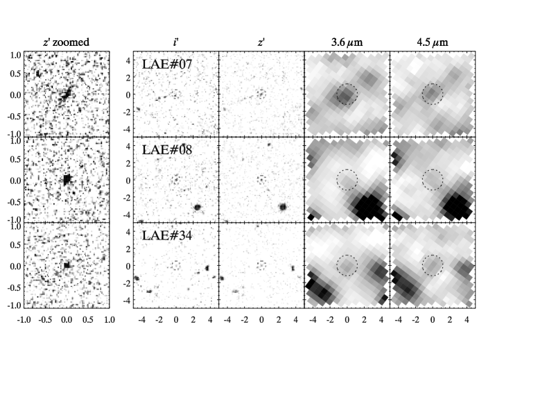
Figure 1.— Images of the three IRAC-detected $z\sim 5.65$ objects in $i^{\prime}$, $z^{\prime}$, 3.6, and 4.5µm. Each panel is 10″across, except for the zoomed $z^{\prime}$ images, which are 2″across. The images are rotated from the original mosaics, when necessary, so that north is up. The ACS stamps are binned with a $3\times 3$ pixels box to bring out the faint extended sources. The full resolution unbinned stamps are shown in the zoomed panels. The circles indicate the apertures used in the photometry measurements.

The star formation history of high-redshift galaxies is an important problem in observational cosmology. It provides tests for galaxy formation theories (e.g. Somerville et al., 2001; Springel & Hernquist, 2003), constrains the sources of reionization (e.g. Barkana & Loeb, 2000, 2001), and may even shed light on the nature of the “first stars” (e.g. Bromm & Larson, 2004).

Recently, the study of star formation at high redshift has been catalyzed by the Infrared Array Camera (IRAC) on board the Spitzer Space Telescope (Fazio et al., 2004). The extraordinary sensitivity of this instrument has enabled the detection of galaxies out to $z\sim 7$. At such high redshifts, optical and near-IR observations accessible to ground based telescopes and the HST sample the rest-frame UV, which provides important information on the on-going star formation and dust extinction. On the other hand, IRAC samples the rest-frame optical light, which is less susceptible to dust extinction and is more representative of the emission from the less massive stars making up the bulk of the stellar population. Infrared observations are therefore indispensable when studying the star formation history of high-redshift galaxies.

Already, a sizable number of IRAC-detected $z\sim 6$ galaxies have been discovered and studied in detail (Dow-Hygelund et al., 2005; Chary et al., 2005; Egami et al., 2005; Eyles et al., 2005; Mobasher et al., 2005; Schaerer & Pelló, 2005; Yan et al., 2005; McLure et al., 2006; Yan et al., 2006). The infrared observations provided by IRAC has allowed the galaxies’ rest-frame UV-to-optical spectral energy distributions (SEDs) to be constrained. Estimates of the masses and ages of the galaxies’ stellar populations can then be obtained. A stunning result from these studies is that many of these high-redshift galaxies are massive ($\gtrsim 10^{10}$ ${\rm M}_{\sun}$), and possess stellar populations that are older than several hundred million years at a time when the age of the universe is less than 1 Gyr.

The vast majority of the IRAC-detected $z\sim 6$ galaxies studied so far have been found using the Lyman break technique (Steidel et al., 1995, 1996, 2003) extended to high redshift (the $i^{\prime}$-dropout technique; Bouwens et al., 2003; Stanway et al., 2003; Yan & Windhorst, 2004). Another, perhaps more efficient, method to search for high-redshift galaxies is to select candidates based on their Ly$\alpha$ emission (Rhoads & Malhotra, 2001; Ajiki et al., 2003; Hu et al., 2004; Malhotra & Rhoads, 2004; Taniguchi et al., 2005). The two methods suffer from different selection biases. For instance, while Ly$\alpha$ searches may allow discovery of sources not detected in the continuum (Fynbo et al., 2001), they may preferentially select young galaxies in a dust-free environment (Malhotra & Rhoads, 2002). In a recent study, Gawiser et al. (2006) found that Ly$\alpha$ emitting galaxies at $z\sim 3$ may be younger and less massive than Lyman break galaxies at similar redshifts. It is therefore interesting to compare the $z\sim 6$ Ly$\alpha$ selected galaxies to the $i^{\prime}$-dropout sample.

In this paper, we present a study of three $z\sim 5.7$ galaxies discovered in the Great Observatories Origins Deep Survey (GOODS; Dickinson et al., 2003) northern field via a narrow-band Ly$\alpha$ survey. Using HST ACS and Spitzer IRAC data from GOODS, we study the rest-frame UV and optical properties of Ly$\alpha$ emitting galaxies at $z\sim 5.7$. The goal is to derive stellar mass and age estimates, and to identify differences, if any, compared to $i^{\prime}$-dropout galaxies at similar redshifts.

The paper is organized as follows. In § 2, we describe the candidate selection strategy and the photometry measurements. In § 3, we present results from population synthesis modeling of the observed SEDs. We compare our sample of Ly$\alpha$ emitting galaxies to the $i^{\prime}$-dropout sample in § 4, and the conclusions are presented in § 5. Hereafter, we will refer to the Ly$\alpha$ emitting galaxies as Ly$\alpha$ emitters (LAEs), and the $i^{\prime}$-dropout galaxies simply as $i^{\prime}$-dropouts. All magnitudes quoted are in the AB magnitude system. We adopt a cosmology of $\{\Omega_{m},\Omega_{\Lambda},h\}=\{0.3,0.7,0.7\}$, consistent with the recent results from WMAP (Spergel et al., 2006).

2. Candidate Selection and Data Reduction

2.1. Candidate Selection and Follow-up Spectroscopy

The high-redshift candidates are selected using a wide-field narrow-band survey. At the time of this paper’s preparation, the survey is being expanded to allow for deeper and more uniform selection criteria over a wider region. Details of the completed survey, selection criteria, and catalog will be presented in an upcoming paper (Hu et al., in prep.). Here we will briefly summarize the portion of the survey and the selection criteria used to construct the current sample.

The narrow-band survey, carried out using SuprimeCam on the Subaru Telescope, covers a 700 arcmin² area encompassing the GOODS northern field. This data set consists of broad-band continuum $UVBRIz^{\prime}$ images (Capak et al. 2004; Hu et al., in prep.), supplemented by narrow-band observations taken with the NB816 filter (Hu et al., in prep.). The NB816 filter has a width of 120 Å FWHM and is centered around 8150 Å, corresponding to Ly$\alpha$ at $z\sim 5.7$.

The narrow-band observations allow for the selection of high-redshift candidates based on the objects’ narrow-band to broad-band flux excess. A detailed discussion of the general selection strategy for $z\sim 5.7$ LAEs can be found in Hu et al. (2004), while considerations specific to this data set are discussed in Hu et al. (in prep.). To summarize, objects with $I-N>0.7$ are selected down to a narrow-band magnitude of $N=25.5$. Due to Ly$\alpha$ forest absorption and the galaxies’ intrinsic continuum break, the high-redshift candidates must also satisfy either a) $R-z^{\prime}>1.8$ and be undetected in $B$ and $V$, or b) be undetected in all passbands redward of $I$.

Candidates satisfying the selection criteria are followed up using the DEIMOS spectrograph on the Keck Telescope. At the DEIMOS resolution, a number of candidates show single asymmetric broad lines, with long red tails and steep blue drop-offs. Such asymmetric lines are characteristic of Ly$\alpha$ emission at high-redshift, and objects displaying such emission lines are classified as $z\sim 5.7$ LAEs.

Our initial sample of spectroscopically confirmed $z\sim 5.7$ LAEs consists of 20 objects (there are additional LAEs from the expanded survey region), with 12 of them falling inside the $10\arcmin\times 16\farcm 5$ region where deep IRAC observations are available from GOODS. Three objects, LAE#07, LAE#08, and LAE#34, show significant emission in the IRAC 3.6 and 4.5 µm channels. From now on, our discussion will be focused on these three IRAC-detected $z\sim 5.7$ LAEs. Spectroscopic redshifts of the objects are tabulated in Table 1. Coordinates, spectra, and Ly$\alpha$ properties for the objects will be presented in an upcoming paper (Hu et al., in prep.) upon completion of the survey.

2.2. X-Ray Nondetection

In order to check for the possibility that our objects are high-redshift AGNs, we turn to the 2 Ms Chandra Deep Field North (CDF-N; Alexander et al., 2003), in which all three of our objects lie. We cross-checked our objects with the point-source catalog by Alexander et al. (2003) and found that none of our objects is detected in that survey. The three IRAC-detected objects lie near the edge of CDF-N, where the sensitivity is lower at $\sim 3\times 10^{-16}$ erg cm^-2 s^-1 (3$\sigma$, full-band 0.5 – 8 keV; see Fig. 18 in Alexander et al. 2003). Nonetheless, a powerful AGN/quasar would have a rest-frame 0.5 – 8 keV luminosity of around $10^{44}$ erg s^-1 (Barger et al., 2003; Brandt & Hasinger, 2005), which translates into an observed 0.5 – 8 keV flux of $4\times 10^{-16}$ erg cm^-2 s^-1 at $z=5.65$ (assuming a photon index $\Gamma=1.8$). Therefore, if our sources were x-ray luminous quasars we would expect to detect them. However, we cannot rule out the possibility of a weak AGN contribution. On the other hand, Wang et al. (2004) surveyed using Chandra a sample of 100 LAEs at $z\sim 4.5$ found by the Large Area Lyman Alpha (LALA) survey, and found no x-ray emission from any of the LAEs. Stacking analysis also reveals no detectable x-ray emission, placing a 3$\sigma$ upper limit on the average 2 – 8 keV luminosity at $L<2.8\times 10^{42}$ erg s^-1. Our objects are selected in a similar manner as the LALA LAEs, and so should be higher redshift counterparts of the LALA objects. Therefore, given the objects’ nondetection in CDF-N and the Wang et al. (2004) results, we consider it unlikely that our objects are high-redshift AGNs.

2.3. Photometry

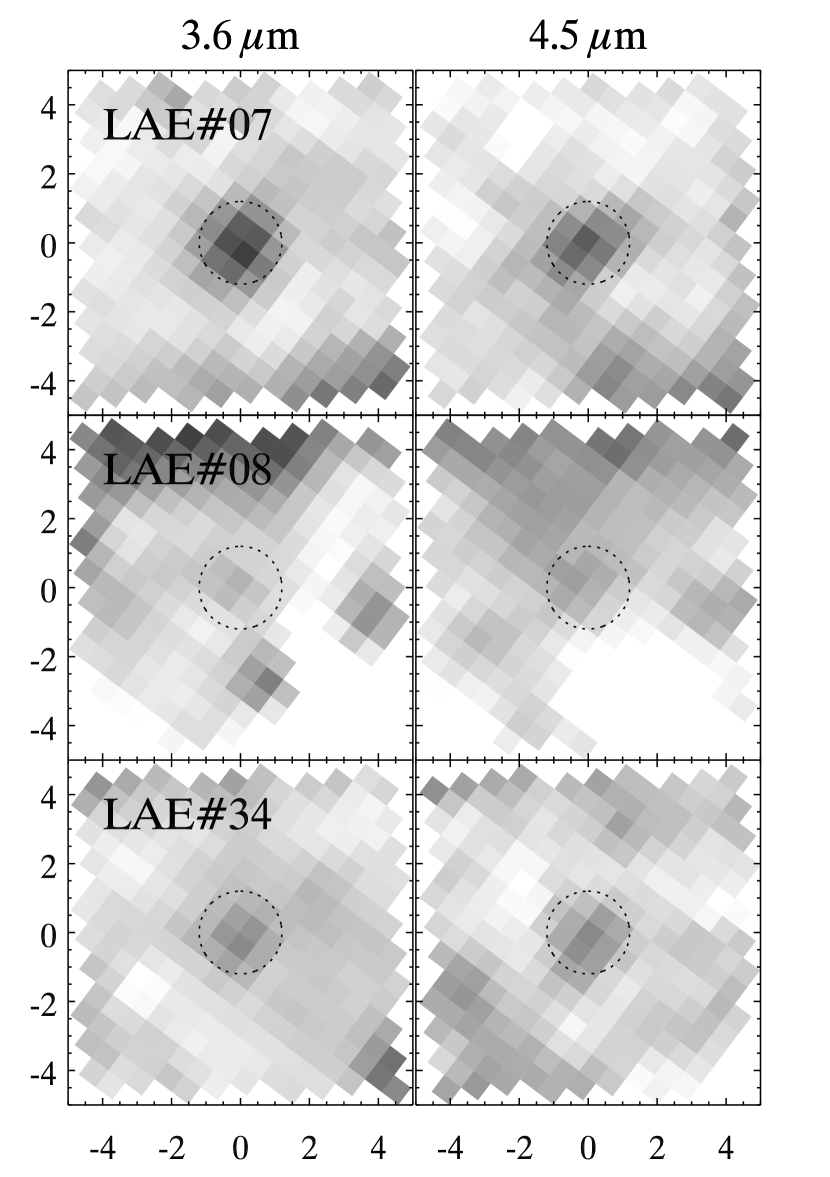
Figure 2.— Object images in the IRAC 3.6 and 4.5 µm bands with the neighboring objects subtracted.

Table 1Measured Flux Densities

	Redshift	$i^{\prime}$		$z^{\prime}$		3.6 µm		4.5 µm
LAE#07	5.635	0.071$\pm$	0.047	0.135$\pm$	0.030	0.53$\pm$	0.20	0.41$\pm$	0.17
LAE#08	5.640	0.070$\pm$	0.045	0.124$\pm$	0.033	0.51$\pm$	0.20	0.61$\pm$	0.17
LAE#34	5.671	0.073$\pm$	0.043	0.091$\pm$	0.025	0.31$\pm$	0.20	0.28$\pm$	0.17

Note. — Flux densities are given in units of $\mu$Jy. Quoted errors are the 1$\sigma$ uncertainties. In the IRAC bands, the errors include systematic uncertainties coming from confusion with neighboring sources. The objects are undetected in $B$, $V$, $R$, 5.8 µm, and 8.0 µm, with 3$\sigma$ upper limits of 0.042, 0.036, 0.063, 1.0, and 1.0 $\mu$Jy, respectively.

The optical photometry is measured from the v1.0 release of the HST ACS data from GOODS. A detailed description of the GOODS ACS data is given in Giavalisco et al. (2004). To summarize, the northern field of GOODS covers an area of $\sim 160$ arcmin² in four passbands: F435W ($B$), F606W ($V$), F775W ($i^{\prime}$) and F850LP ($z^{\prime}$). The images have PSF FWHM $\sim 0\farcs 12$ and reach depths of 27.4, 27.5, 26.8, and 26.5 mag ($3\sigma$ in 1″-diameter apertures) in the $B$, $V$, $i^{\prime}$, and $z^{\prime}$bands, respectively.

Infrared coverage is provided by deep Spitzer IRAC observations, covering the same field as the ACS imaging, obtained as part of the GOODS program (Dickinson et al., in prep.). The data consist of imaging in four passbands, centered at 3.6, 4.5, 5.8 and 8.0 µm. The IRAC photometry are measured using images from our own independent reduction of the GOODS data. The $3\sigma$ magnitude limits (in 2$\farcs$4-diameter apertures) in our images are 26.2, 26.4, 25.0, and 25.1 mag in the 3.6, 4.5, 5.8, and 8.0 µm bands, respectively. The PSF FWHM is $\sim 2\arcsec$ on average, but is slightly better at $\sim 1\farcs 8$ in the 3.6 and 4.5 µm bands.

The three objects are detected only in the $i^{\prime}$, $z^{\prime}$, 3.6 µm, and 4.5 µm bands. Stamp images of the objects in these four passbands are shown in Figure 1. LAE#07 and LAE#08 appear to be marginally resolved in the ACS images, with approximate angular sizes of $\sim 0\farcs 7$ and 0$\farcs$35, respectively. Taken at face value, the angular sizes correspond to physical sizes of $\sim$ 4 and 2 kpc for LAE#07 and LAE#08.

We perform aperture photometry on the ACS images for each of the three objects. Because of the extended nature of the objects in the ACS images, extra care has to be taken when selecting the appropriate aperture size. We adopt a 1″-diameter aperture in the measurements. Curve of growth analysis of the three objects suggests that $\lesssim 1\%$ of the total flux fall outside an 1″-diameter aperture. While a large aperture is not ideal for minimizing background noise contributions, it is necessary in order to measure the total flux of the objects. Since the fraction of enclosed flux within our chosen aperture is close to unity, and the objects are intrinsically faint and extended, we opted not to apply aperture corrections to the photometry.

Photometry measurements on the IRAC images are considerably more challenging. At the IRAC resolution, all three objects are unresolved and can be treated as point sources. However, because of the large PSF, neighboring objects may significantly contaminate the photometry. For example, LAE#07 is heavily blended with two other faint neighbors, while LAE#08 is located in the wings of a bright foreground galaxy (Fig. 1).

To address this problem, we use a deblending technique whereby the contaminating neighbors are subtracted using the high resolution ACS images convolved with the IRAC PSF. We use the ACS $z^{\prime}$-band image as input since it is the closest to the IRAC bands in wavelength and the objects are brightest in this passband. In fact, we in general use the $z^{\prime}$-band image as the reference for object positions. The IRAC PSF is obtained directly from the images by stacking $\sim 10$ bright point sources within the field.

For each contaminating object in the vicinity of the target, the $z^{\prime}$-band image is convolved with the IRAC PSF. Then, after first subtracting all the neighboring sources using the current best-fits, the convolved image of the contaminating object is fitted to its IRAC counterpart. The parameters fitted for are the object’s amplitude, background, and position. This process is iterated until a converged solution for every contaminating object is found. Using the best-fit solution, the contaminating objects are subtracted from the original IRAC image, leaving only the target. The result of this deblending procedure is shown in Figure 2. It is important to note that this deblending procedure works best when the objects to be subtracted are unresolved, such as the neighbors of LAE#07. The procedure is less successful in subtracting the bright extended foreground galaxy neighboring LAE#08, most likely due to uncertainties and spatial variations in the IRAC PSF, and possible wavelength dependence in the foreground galaxy’s morphology. Nonetheless, Figure 2 shows that the deblending procedure works quite well in removing contamination from neighboring sources.

After the contaminating neighbors are subtracted from the IRAC images, we measure the objects’ photometry in 2$\farcs$4-diameter apertures, centered at the positions derived from the $z^{\prime}$-band images. The aperture size is chosen to be as small as possible to minimize background noise and residual flux from nearby objects. Aperture corrections factors of $\sim 0.5$ are applied to the measured fluxes.

Uncertainties in the ACS photometry are estimated using a Monte-Carlo procedure. Artificial point sources, with fluxes equal to the objects, are inserted into the images. The positions of the artificial sources are assigned randomly apart from the requirement that they are at least 1 aperture diameter away from detected sources. We then apply the same measurement procedure we used on the objects to the artificial sources. The resulting dispersion in the measured fluxes will serve as an estimate of the uncertainties in the objects’ photometry. This procedure provides an estimate of the errors introduced by sky fluctuations and sky subtraction, and it takes into account the correlations between adjacent pixels introduced by the drizzle procedure used to produce the ACS mosaics. The errors derived in this way also include the confusion noise due to faint undetected sources.

For the IRAC images, there is an additional source of error coming from the neighbor subtraction. Ideally, we would apply a similar Monte-Carlo procedure, repeating the neighbor subtraction process many times on artificial sources to obtain the error estimates. However, the convolution-based neighbor subtraction process is time-consuming, and so a full Monte-Carlo approach is impractical.

We therefore try to mimic the effects of neighbor subtraction using the PSF-fitting package StarFinder (Diolaiti et al., 2000). The errors in the source subtraction are dominated by image quality issues, such as variations of the PSF across the field, and by the properties of the individual sources (e.g. deviations from being perfect point sources). The differences in the source subtraction using StarFinder and our convolution-based procedure should be small compared to the aforementioned uncertainties. Hence, we believe that performing the source subtraction using StarFinder will give a reasonable estimate of the errors introduced by our convolution-based neighbor subtraction process.

Using StarFinder, sources are detected and subtracted from the IRAC images. Artificial sources are inserted randomly into the source subtracted image and their fluxes are then measured. Any errors arising from the imperfect source subtractions, as well as the statistical errors coming from the background and its subtraction, would be included in the resulting measured flux dispersion. The IRAC photometry errors thus derived are conservative since we expect our convolution-based subtraction to perform better than StarFinder in the case where the objects are not perfect point sources. Also, the artificial sources are placed purely randomly throughout the image, so they may overlap subtracted sources. This tends to overestimate the uncertainties since the errors in the subtraction are larger near the center of the sources where the flux is higher. The results of the flux measurements and error estimates described above are summarized in Table 1.

Finally, we supplement the ACS and IRAC imaging using data from the Hawaii-HDF-N project (Capak et al., 2004). We attempt to measure the objects’ photometry in the $R$-band images from Subaru and the HK^′ images from the UH 2.2m telescope. However, these images are shallower than the ACS and IRAC data, and none of the objects are detected (in 3″-diameter apertures) in either $R$ or HK^′. We include the $R$-band upper limit (27.2 mag, 3$\sigma$) in our analysis for completeness. The HK^′-band upper limit (22.7 mag, 3$\sigma$) is too high to make a difference in the following analysis, and is therefore omitted.

3. Spectral Energy Distribution and Stellar Population

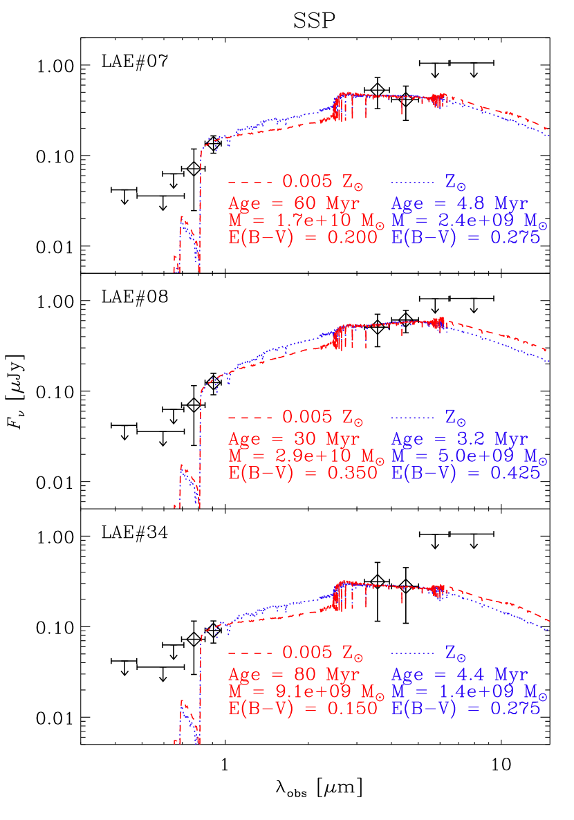
Figure 3.— Best fit SSP models to the three IRAC-detected $z\sim 5.7$ LAEs. The blue-dotted (red-dashed) line is for a model with $Z={\rm Z}_{\sun}$ (0.005 ${\rm Z}_{\sun}$). The observed SEDs are plotted as diamonds with error bars. The horizontal error bars indicate approximately the FWHM of the passbands. When an object is undetected in a certain passband, the corresponding 3$\sigma$ upper limit is shown. Note that a 30% fractional error is added to the $i^{\prime}$-band to account for the Ly$\alpha$ line contribution.

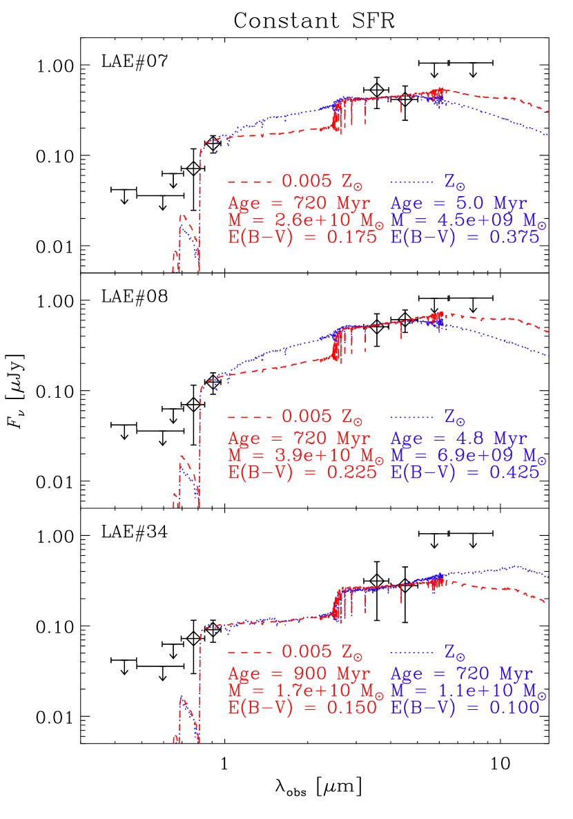
Figure 4.— Best fit constant SFR models to the three IRAC-detected $z\sim 5.7$ LAEs. Symbols and line styles have the same meaning as in Figure 3.

3.1. Population Synthesis Modeling

After we have obtained reliable photometry for the galaxies, we use the stellar population synthesis model of Bruzual & Charlot (2003, hereafter BC03) to model the galaxies’ SEDs. The basic strategy is to calculate model SEDs, varying the mass, age, dust reddening, metallicity, and star formation history. The model SEDs are redshifted and integrated through the filter response function. The model predictions are then compared to the observed photometry and the best-fitting model is found by $\chi^{2}$ minimization.

For simplicity, and to facilitate comparison with other works in the literature, we will assume throughout this study the Salpeter (1955) initial mass function (IMF), implemented in the BC03 models with lower and upper mass cutoffs of 0.1 and 100 ${\rm M}_{\sun}$. We will discuss the effects of using a different IMF and other variations in the population synthesis models in § 3.3. We explore models with five different metallicities: Z/${\rm Z}_{\sun}$ = 0.005, 0.02, 0.2, 0.4, and 1. Note that metallicity is not treated as a free parameter in the fitting process, but rather an input assumption of the model. The effect of dust reddening is included using the Calzetti et al. (2000) model, with $E(B-V)$ varying between 0.0 – 1.0. The effect of Ly$\alpha$ forest attenuation is included using the model of Madau (1995). There is no need to fit for the objects’ redshifts, since these are known from spectroscopy. An additional constraint arising from the known redshifts is that the inferred ages should not exceed the age of the universe, which is approximately 0.99 Gyr at $z\sim 5.65$. We therefore impose an upper limit of 0.9 Gyr on the age of the best-fit models.

The star formation history (SFH) is parameterized by the time evolution of the star formation rate (SFR). We consider two SFHs in our analysis: Simple Stellar Population (SSP), i.e. instantaneous burst, and constant SFR. We choose not to consider more complicated SFHs, such as an exponentially declining SFR, because our ability to constrain extra parameters is limited. All our objects are detected in only four passbands, so we can constrain up to three parameters, which we choose to be mass, age, and dust reddening $E(B-V)$. Using an exponential SFR would introduce an extra parameter, the star formation timescale $\tau$, which can be constrained only if we fix the value of another parameter such as $E(B-V)$. We will return to this point later in § 3.3. Note that the SFHs used in our analysis (SSP and constant SFR) represent the two extremes in star formation timescales, and an exponential SFR can be thought of as an intermediate between these two examples.

With two SFHs and five metallicities, there are 10 different classes of models in total. The best-fitting model within each class is found by $\chi^{2}$ minimization. There are three free parameters (mass, age, and reddening) and four data points ($i^{\prime}$, $z^{\prime}$, 3.6 µm, and 4.5 µm), resulting in 1 degree of freedom in the $\chi^{2}$ fits. In practice, a commonly used measure of the goodness of fit is $\chi_{\nu}^{2}$, the $\chi^{2}$ per degree of freedom. When $\nu=1$, a model is rejected at the 1, 2, and 3-$\sigma$ levels if $\chi_{\nu}^{2}$ is larger than 1, 4, and 9, respectively. We in general consider a fit to be acceptable if it gives $\chi_{\nu}^{2}<4$. In certain cases when $\nu=2$ (see § 3.2), a fit is deemed acceptable if $\chi_{\nu}^{2}<3.09$ (the corresponding 2$\sigma$ level for $\nu=2$).

In order to make full use of the data available, we incorporate undetected data points as follows. Given the detection limit of the exposure $\sigma$ and the model flux in the channel $\mu$, we calculate the probability $I=P(<\sigma|\mu)$ that the actual flux of the object is less than $\sigma$. For the purpose of this calculation, the flux is assumed to be normally distributed with mean $\mu$ and width $\sigma$. For each undetected channel, a value of $-\ln(I)$ is then added to the total $\chi^{2}$. In this way, if the model flux is much higher than the detection limit, $\mu\gg\sigma$, $I$ would be small and the model would incur a large $\chi^{2}$ penalty. For example, if the model flux in a certain channel is at the $3\sigma$ detection limit, $\mu=3\sigma$, the $\chi^{2}$ penalty would be 3.8. In practice, the undetected data points have only a small effect on the total $\chi^{2}$, since the detection limits in most channels can easily be satisfied by reasonable models.

Since the Ly$\alpha$ emission line is located inside the $i^{\prime}$-band at $z\sim 6$, and the BC03 model does not predict emission line strengths, we have to take into account the possible Ly$\alpha$ line emission when fitting to the data. The fractional contribution of the line to the broad-band flux can be approximated as $F_{L}/F_{B}=(R-1)W_{N}/W_{B}$, where $W_{N}/W_{B}$ and $R=F_{\nu}(N)/F_{\nu}(B)$ are the ratios of the narrow-band to broad-band widths and flux densities, respectively. Our objects are selected based on their narrow-band to broad-band flux excess, and typically have $N-I\sim-1.5$. Substituting $W_{N}\approx 120$ Å and $W_{B}\approx 1400$ Å for the NB816 and $I$ filters, and $R=10^{-0.4(N-I)}\approx 4$, we find that the Ly$\alpha$ line may contribute around 30% of the total $I$-band flux. Note that this approximation implicitly assumes that the Ly$\alpha$ forest truncates similar fractions of the narrow-band and broad-band fluxes. Since Ly$\alpha$ at $z\sim 5.7$ is located slightly redward of the $i^{\prime}$-band center, Ly$\alpha$ forest truncation affects the $i^{\prime}$-band flux more severely than $I$ or NB816. The Ly$\alpha$ line contribution may therefore be substantially higher than 30% in the $i^{\prime}$-band. Nevertheless, we add an optimistic 30% fractional error to the $i^{\prime}$-band flux when we perform the $\chi^{2}$ fits.

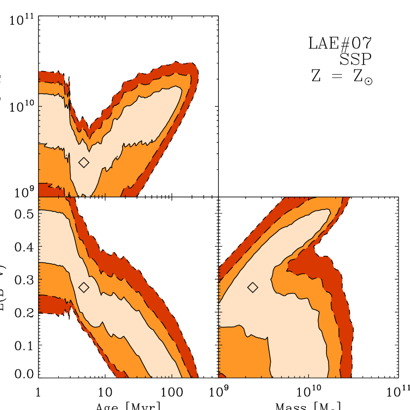
Figure 5.— $\Delta\chi^{2}$ contour for LAE#07 in the ${\rm Z}_{\sun}$ SSP model. The diamond marks the best fitting model. The solid, long-dashed, and short-dashed lines represent the 1, 2, and 3-$\sigma$ confidence regions.

3.2. Fitting Results

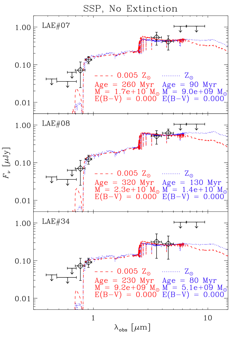
Figure 6.— Best fit SSP models to the three IRAC-detected $z\sim 5.7$ LAEs with fixed $E(B-V)=0$. Symbols and line styles have the same meaning as in Figure 3.

Table 2Best-Fit Model Parameters

	Age [Myr]	Mass [${\rm M}_{\sun}$]		$E(B-V)$	$\chi_{\nu}^{2}$		Age [Myr]	Mass [${\rm M}_{\sun}$]		$E(B-V)$	$\chi_{\nu}^{2}$
	SSP, ${\rm Z}_{\sun}$						SSP, 0.005 ${\rm Z}_{\sun}$
LAE#07	4.8	2.4$\times$	$10^{9}$	0.275	2.05		60	1.7$\times$	$10^{10}$	0.200	1.97
LAE#08	3.2	5.0$\times$	$10^{9}$	0.425	2.19		30	2.9$\times$	$10^{10}$	0.350	2.20
LAE#34	4.4	1.4$\times$	$10^{9}$	0.275	2.42		80	9.1$\times$	$10^{9}$	0.150	2.36
	Constant SFR, ${\rm Z}_{\sun}$						Constant SFR, 0.005 ${\rm Z}_{\sun}$
LAE#07	5.0	4.5$\times$	$10^{9}$	0.375	2.14		720	2.6$\times$	$10^{10}$	0.175	2.19
LAE#08	4.8	6.9$\times$	$10^{9}$	0.425	2.19		720	3.9$\times$	$10^{10}$	0.225	2.18
LAE#34	720	1.1$\times$	$10^{10}$	0.100	2.47		900	1.7$\times$	$10^{10}$	0.150	2.37
	SSP, ${\rm Z}_{\sun}$, No Extinction						SSP, 0.005 ${\rm Z}_{\sun}$, No Extinction
LAE#07	90	9.0$\times$	$10^{9}$	0.000	1.25		260	1.7$\times$	$10^{10}$	0.000	1.05
LAE#08	130	1.4$\times$	$10^{10}$	0.000	1.45		320	2.3$\times$	$10^{10}$	0.000	1.28
LAE#34	80	5.1$\times$	$10^{9}$	0.000	1.41		230	9.2$\times$	$10^{9}$	0.000	1.27

The observed SEDs of the three galaxies are shown in Figure 3. Ignoring the lines for the moment, the first thing to take note is that all three galaxies exhibit similar rest-frame UV and optical emission properties. This is not surprising since the three objects are selected from same data set using the same selection criteria. The galaxies’ SEDs are characterized by red UV to optical colors, with the flux increasing by more than a factor of 3 from $z^{\prime}$ to 3.6 µm. The SEDs also show signs of flattening out beyond 3.6 µm.

The best fit BC03 models to the observed SEDs are shown in Figure 3 and Figure 4 for the SSP and constant SFR models, respectively. Only models with the two extreme metallicities (${\rm Z}_{\sun}$ and 0.005 ${\rm Z}_{\sun}$) are shown, even though fits were performed for all five possible metallicities. In practice, we find good fits with competitive $\chi^{2}$ for all five metallicities. Note that the $i^{\prime}$-band flux is consistently higher than the models, owing to the Ly$\alpha$ line emission. Also, since the $i^{\prime}$-band straddles the Lyman-break, the model band-integrated flux is larger than it seems, and is usually within 1$\sigma$ of the observed value.

The best-fit parameters differ depending on the SFH and metallicity (Table 2). The best-fit ${\rm Z}_{\sun}$ SSP models to the three LAEs have ages $\sim 5$ Myr, masses $\sim 5\times 10^{9}$ ${\rm M}_{\sun}$, and $E(B-V)\sim 0.3-0.4$. The best-fit 0.005 ${\rm Z}_{\sun}$ SSP models favor slightly older ages ($\sim 50$ Myr), larger masses ($\sim 10^{10}$ ${\rm M}_{\sun}$), and somewhat lower extinction. This is mostly because metal-poor stars produce more UV photons, so the best-fit models need to be older in order to match the red UV-to-optical colors in the data. These results suggest that our sample of $z\sim 5.7$ LAEs displays qualities of dusty young galaxies, seen immediately after or during a burst of star formation.

Compared to the SSP models, the constant SFR models in general yield older ages at $\gtrsim 700$ Myr and slightly larger masses at a few times $10^{10}$ ${\rm M}_{\sun}$. In some cases, however, the best-fit constant SFR models have similar parameter values as the SSP models. This is not surprising since for young ages the constant SFR model is similar to the SSP model.

Given that we only have four data points, some of which have fairly large error bars, it is important to explore the range of models allowed by the data. Furthermore, the somewhat high levels of extinction we obtained may seem be a little surprising. Several previous studies have found little or no dust extinction in $z\sim 6$ $i^{\prime}$-dropouts (Dow-Hygelund et al., 2005; Eyles et al., 2005; Mobasher et al., 2005; Yan et al., 2005). The fact that our galaxies are selected based on their Ly$\alpha$ emission would also lead one to expect low extinction values, since Ly$\alpha$ photons are very susceptible to dust scattering (Charlot & Fall, 1991; Chen & Neufeld, 1994; Hansen & Oh, 2006). Do the data permit models with low extinction? What is the range of age and mass allowed by the data?

To answer these questions, we calculate confidence regions for the best-fit parameters. In Figure 5, we show the $\Delta\chi^{2}$ contours for LAE#07 in the ${\rm Z}_{\sun}$ SSP model. It can be seen from the figure that firm upper limits on the age and mass can be placed on LAE#07. In the context of the SSP model, LAE#07 has a mass of $\lesssim 3\times 10^{10}$ ${\rm M}_{\sun}$, and an age of $\lesssim 300$ Myr. The contours and limits for the other two objects are similar.

One important thing to note in Figure 5 is that there is a range of models that fits the data. This is the result of a fundamental degeneracy in the models: the red UV-to-optical colors of the observed SEDs can be satisfied by either a significant Balmer break (implying a relatively mature stellar population), or a young stellar population with high extinction. Figure 5 shows that even though the best-fit model has a young age and high extinction, there are models with lower extinction values and older ages that will fit the data equally well.

Because of this degeneracy, we performed an alternative fit to the data forcing $E(B-V)=0$. The results of this fit for the SSP model are presented in Figure 6. Good fits to the data can be obtained for all metallicities. The best-fit models to the three galaxies in the ${\rm Z}_{\sun}$ case have masses $\sim 10^{10}$ ${\rm M}_{\sun}$, and ages $\sim 100$ Myr. The 0.005 ${\rm Z}_{\sun}$ model gives older ages (around a few hundred Myr) and slightly larger masses. In general, the no extinction models have a lower $\chi_{\nu}^{2}$ (see Table 2), mostly due to the extra degree of freedom ($\nu=2$ in this case). Note that in the SSP models presented here, there will not be enough young massive stars around to produce significant Ly$\alpha$ emission becuase of the older ages. The results we obtained should therefore be regarded as a fit to the older stellar population that dominates the total mass of the system. The observed Ly$\alpha$ emission can still be explained by the presence of a young but significantly less massive stellar population within the galaxy. We find no satisfactory constant SFR models with $E(B-V)=0$. Without dust extinction, these models produce too much UV compared to the data.

In a recent study, Le Delliou et al. (2006) made detailed predictions of the properties of LAEs, based on a hierarchical galaxy formation model. We find that the best-fit stellar masses of our LAEs are about 1 – 2 orders of magnitude larger that the values predicted by Le Delliou et al. (2006). The most probable reason for this discrepancy is that a top heavy IMF is used in Le Delliou et al. (2006), resulting in a lower M/L ratio and hence lower overall mass. By requiring that our LAEs be detected by IRAC, we may also be selecting galaxies from the high-mass end of the distribution (§ 4.2). Other properties of the LAEs, such as the broad-band magnitudes as a function Ly$\alpha$ flux, agree quite well with the predictions of the Le Delliou et al. (2006) model.

In summary, we find that the three IRAC-detected $z\sim 5.7$ LAEs in our sample show similar emission properties and can be fitted with similar model SEDs. The current data are unable to distinguish between models with different metallicities, as best-fit models with competitive $\chi^{2}$ can be found for all metallicities. The observed SEDs are broadly consistent with two classes of models. In one model, the galaxies are dusty, young (ages $\lesssim 100$ Myr), and relatively less massive ($M\sim 10^{9}$ ${\rm M}_{\sun}$). In the other model, the galaxies are less dusty, more massive ($M\sim 10^{10}$ ${\rm M}_{\sun}$), and older ($\gtrsim 100$ Myr) with a significant Balmer break. Both types of models can provide satisfactory fits to the data. This degeneracy stems from the fact that we only have two data points ($i^{\prime}$ and $z^{\prime}$) with which to measure the UV spectral slope, which is sensitive to both dust extinction and metallicity. Very deep near-IR observations in the $J$, $H$, or $K$ bands would provide valuable constraints on the UV spectral slope, and may help to break the degeneracy and rule out some of the possible models.

3.3. Alternative Models

In addition to the basic models discussed in the previous section, we also tried to fit a number of alternative models to the data, in order to explore several effects not included in the basic fits. These alternative models are discussed in turn below.

Exponential SFR. — We did not consider an exponential SFR in our basic fits because with only four data points, it is not possible to fit for the mass, age, reddening, and star formation timescale ($\tau$) simultaneously. However, if we are willing to sacrifice one degree of freedom in another parameter, we can attempt to fit an exponential SFR model to the data. In the previous section, we found that the galaxies can be fitted by models with very little dust extinction. Other studies of galaxies at similar redshifts also found little or no dust extinction (Dow-Hygelund et al., 2005; Eyles et al., 2005; Mobasher et al., 2005; Yan et al., 2005). We therefore attempt to fit an exponential SFR model with $E(B-V)$ fixed at zero. Good fits to the data can be found using all metallicities, with $\tau$ on the order of 400 Myr. Since the best-fit $\tau$ is fairly large, the exponential model is not unlike the Constant SFR model. In fact, the two SFH models give similar masses and ages, which are $\sim 10^{10}$ ${\rm M}_{\sun}$ and $\sim 700$ Myr, respectively.

Chabrier IMF. — In addition to the Salpeter IMF, the Chabrier (2003) IMF is also implemented in the BC03 models. The Chabrier IMF has a flatter distribution than Salpeter at $<$ 1 ${\rm M}_{\sun}$. Stars more massive than 1 ${\rm M}_{\sun}$ therefore have a larger relative contribution to the total luminosity, resulting in a lower $M/L$ ratio. Hence, the Chabrier IMF in general produces best-fit stellar masses that are $\sim 30\%-40\%$ lower than the Salpeter IMF.

Alternative Population Synthesis Model. — An alternative population synthesis model was recently introduced by Maraston (2005). The main new ingredient of this model is an increased emphasis on the contributions of thermally pulsating asymptotic giant branch (TP-AGB) stars to the overall luminosity. Contributions from TP-AGB stars are strongest in stellar populations around $\sim 1$ Gyr old, and their effect is to raise the luminosity at near-IR and longer wavelengths. In general, this results in a lower $M/L$ ratio, and hence smaller best-fit masses and ages (Mobasher et al., 2005; Maraston et al., 2006). However, since the LAEs in our sample are in general much younger than 1 Gyr, and we have data available only in the rest-frame optical and shorter wavelengths, we do not expect the Maraston (2005) model to give significantly different results than the BC03 model. On the other hand, TP-AGB stars could potentially contribute to the 5.8 and 8.0 µm flux of $z\sim 6$ galaxies, and we stress that it is important to investigate this alternative model in cases where 5.8 and 8.0 µm data are available.

4. Comparison to the $i^{\prime}$-dropout Sample

One of the main goals of this study is to compare and contrast the properties of the $z\sim 6$ IRAC-detected LAEs and $i^{\prime}$-dropouts. As we have mentioned in § 1, the different selection criteria for LAEs and $i^{\prime}$-dropouts may imply fundamental physical differences between these two populations. One thing we try to accomplish is to compare the two populations using model-independent empirical indicators of the galaxies’ properties, such as the rest-frame UV-to-optical color. Our sample of IRAC-detected $z\sim 6$ $i^{\prime}$-dropouts is drawn from the works of Dow-Hygelund et al. (2005), Eyles et al. (2005), and Yan et al. (2005). Other objects are not included either because they lie at higher redshifts ($z\gtrsim 6.5$) so accurate $i^{\prime}-z^{\prime}$ color cannot be measured owing to Ly$\alpha$ forest attenuation, or because IRAC photometry is not available.

4.1. $i^{\prime}-z^{\prime}$ color

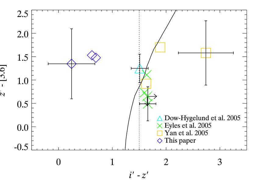
Figure 7.— $z^{\prime}-[3.6]$ vs. $i^{\prime}-z^{\prime}$ colors of the LAEs in this paper and other IRAC-detected $z\sim 6$ $i^{\prime}$-dropouts in the literature. Only the error bars of the object with the faintest $z^{\prime}$ magnitude in each group are shown. This is done to avoid clutter and to provide a conservative estimate of the errors associated with each group of measurements. The vertical dotted line corresponds to $i^{\prime}-z^{\prime}=1.5$, a typical selection criterion for the $z\sim 6$ $i^{\prime}$-dropouts. The curve shows the color evolution of a dust-free, 0.005 ${\rm Z}_{\sun}$, SSP mode. The curve corresponds to model ages from $\sim 30$ Myr near the bottom of the plot to $\sim 800$ Myr near the top.

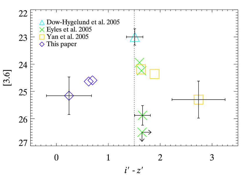
Figure 8.— IRAC 3.6 µm magnitude vs. $i^{\prime}-z^{\prime}$ color of the LAEs in this paper and other IRAC-detected $z\sim 6$ $i^{\prime}$-dropouts in the literature.

The $z^{\prime}-[3.6]$ color is plotted against the $i^{\prime}-z^{\prime}$ color in Figure 7 for both our LAEs and the $z\sim 6$ $i^{\prime}$-dropouts. The most striking feature in Figure 7 is that the LAEs have much bluer $i^{\prime}-z^{\prime}$ color than the $i^{\prime}$-dropouts. In fact, all three LAEs in our sample have $i^{\prime}-z^{\prime}$ colors that are well blueward of the typical $i^{\prime}$-dropout selection criterion of $i^{\prime}-z^{\prime}>1.5$. One possible reason for this difference is that the $i^{\prime}$-dropouts are preferentially selected to have red $i^{\prime}-z^{\prime}$ color, which may also result in the $i^{\prime}$-dropouts being selected at slightly higher redshifts than the LAEs. Another reason is the unusually high $i^{\prime}$-band flux observed in our sample (c.f. § 3.2), which may be explained by the Ly$\alpha$ line contribution. We have remarked in § 3.1 that the Ly$\alpha$ line can contribute $\sim 30\%$ or more of the total broad-band flux. In addition, Hu et al. (2004) found that, in a sample of LAEs selected in a similar manner as our objects, there is a clear correlation between the narrow-band and $I$-band magnitudes, and that all of the spectroscopically identified LAEs in the sample have $I-z^{\prime}<1.5$ (see their Fig. 5). Similarly, we find that all three of the LAEs have $i^{\prime}-z^{\prime}<1.5$.

The blue $i^{\prime}-z^{\prime}$ colors of the LAEs in our sample implies that they would have been overlooked by previous surveys based on the $i^{\prime}$-dropout selection criterion. It is therefore important to understand the overlap between the LAE and $i^{\prime}$-dropout galaxies, so that the properties of the overall $z\sim 6$ galaxy population, such as the total stellar mass density, can be constrained.

4.2. Stellar Population

At $z\sim 6$, the $z^{\prime}$ and IRAC 3.6 µm bands sample the rest-frame UV and optical light, respectively. If we ignore the effects of dust extinction, the $z^{\prime}$ magnitude is sensitive to the massive young stars in the galaxy, while the 3.6 µm magnitude measures the contributions from less massive, evolved stars. The $z^{\prime}-[3.6]$ color, plotted against the $i^{\prime}-z^{\prime}$ color in Figure 7, is therefore an indicator of the age of the stellar population. The model color evolution, also plotted in Figure 7, help to illustrate this point. The curve starts at $\sim 30$ Myr near the bottom of the plot. As the age increases, $z^{\prime}-[3.6]$ also increases, and eventually reaching $z^{\prime}-[3.6]=2.5$ at an age of $\sim 800$ Myr.

As we have mentioned before, the presence of Ly$\alpha$ emission may signal a young stellar population. However, Figure 7 shows that there is no significant difference between the $z^{\prime}-[3.6]$ color of the LAEs and that of the $i^{\prime}$-dropouts. Therefore, we find no evidence to suggest that there is a systematic age difference between the IRAC-detected LAE and $i^{\prime}$-dropout populations. However, we stress again that the $z^{\prime}-[3.6]$ color is a good indicator of stellar population age only in the absence of dust.

Figure 8 shows the 3.6 µm band magnitude plotted against $i^{\prime}-z^{\prime}$. All objects in Figure 8 lie at similar redshifts, and hence similar luminosity distances. This implies the 3.6 µm magnitude may serve as a measure of the total evolved stellar mass in the galaxies. The 3.6 µm magnitudes of the LAEs fall comfortably inside the range of magnitudes observed for the $i^{\prime}$-dropouts. Therefore, we again find no evidence that the IRAC-detected LAEs and $i^{\prime}$-dropouts are systematically different.

In terms of stellar population synthesis modeling, the results are consistent as well. For the $z\sim 6$ $i^{\prime}$-dropouts, stellar population synthesis modeling in general gives ages around a few hundred Myr, and masses around $10^{10}$ ${\rm M}_{\sun}$. This is mostly in line with the values we obtained for the LAEs (Table 2), at least in the dust-free SSP case.

It is important to keep in mind the comparison presented here is restricted to the IRAC-detected LAEs and $i^{\prime}$-dropouts. By requiring IRAC detection for the galaxies, the selection is biased towards the bright end of the luminosity function. Recent studies of $i^{\prime}$-dropouts at $z\sim 6$ suggest that the IRAC-invisible galaxies are in general younger and less massive (Eyles et al., 2006; Yan et al., 2006). Gawiser et al. (2006) also found that LAEs at $z=3.1$ typically have lower masses at $\sim 5\times 10^{8}$ ${\rm M}_{\sun}$. The similarities seen in Figure 7 and Figure 8 may therefore be a result of this IRAC-selection bias.

5. Conclusion

In this paper, we studied in detail the properties of three Ly$\alpha$ emitting galaxies, each spectroscopically confirmed to lie at $z\sim 5.65$. Using ACS and IRAC data from GOODS, we measured the galaxies’ SEDs in the rest-frame UV through optical. Stellar population synthesis modeling then allows us to place constraints on the galaxies’ masses and ages. Our main conclusions may be summarized as follows.

The three IRAC-detected LAEs in our sample exhibit similar emission properties, characterized by a red rest-frame UV-to-optical color, with the flux increasing by more than a factor of 3 from $z^{\prime}$ to 3.6 µm. This feature can be explained by a young stellar population with significant dust extinction, or an older stellar population that has developed a Balmer break. Assuming the SSP model for the star formation history, we find best-fit stellar populations with masses between $\sim 10^{9}-10^{10}$ ${\rm M}_{\sun}$ and ages between $\sim 5-100$ Myr. However, stellar populations as old as 700 Myr are admissible if a constant SFR model is considered. Very deep near-IR observations may help to narrow the range of allowed models by providing extra constraints on the rest-frame UV spectral slope. The available data provide very little constraints on the LAEs’ metallicity. We fitted stellar population synthesis models using five metallicities ranging from 0.005 ${\rm Z}_{\sun}$ to ${\rm Z}_{\sun}$, and found that equally good fits with similar parameter values can be obtained for all metallicities.

In comparison with other IRAC-detected $z\sim 6$ galaxies selected based on the $i^{\prime}$-dropout technique, we find that the LAEs and $i^{\prime}$-dropouts possess similar $z^{\prime}-[3.6]$ colors, suggesting that they are similar in ages. Also, the LAEs and $i^{\prime}$-dropouts have comparable 3.6 µm magnitudes, which imply they have similar masses. On the other hand, the comparison is restricted to the IRAC-detected LAEs and $i^{\prime}$-dropouts, which are likely to be the brightest and most massive members of their respective populations. The observed similarities between the IRAC-detected LAEs and $i^{\prime}$-dropouts may be a result of this selection bias.

Even though the IRAC-detected LAEs and $i^{\prime}$-dropouts share some common characteristics, the LAEs have much bluer $i^{\prime}-z^{\prime}$ colors. Many previous searches for $z\sim 6$ galaxies were based on a combination of $i^{\prime}-z^{\prime}$ color selection and non-detections in bands blueward of $i^{\prime}$. Because of their blue $i^{\prime}-z^{\prime}$ colors, LAEs would be overlooked by these searches unless additional selection criteria are incorporated. One present challenge is therefore to understand the overlap between the LAE and $i^{\prime}$-dropout populations. The solution to this problem will shed light on the $z\sim 6$ galaxy population in general, and help to constrain the total stellar mass density, as well as the total contribution of massive galaxies to the ionization background at $z\sim 6$.

We would like to thank the referee, Matt Malkan, for insightful comments that improved the paper. We also thank Eric Gawiser and Haojing Yan for helpful discussions. EMH acknowledges suport from NSF grant AST06-87850 and LLC from AST04-07374. This work is based in part on observations made with the Spitzer Space Telescope, which is operated by the Jet Propulsion Laboratory, California Institute of Technology under a contract with NASA. Support for this work was provided by NASA.

References

- Ajiki et al. (2003) Ajiki, M., et al. 2003, AJ, 126, 2091
- Alexander et al. (2003) Alexander, D. M., et al. 2003, AJ, 126, 539
- Barger et al. (2003) Barger, A. J., et al. 2003, AJ, 126, 632
- Barkana & Loeb (2000) Barkana, R. & Loeb, A. 2000, ApJ, 539, 20
- Barkana & Loeb (2001) —. 2001, Phys. Rep., 349, 125
- Bouwens et al. (2003) Bouwens, R. J., et al. 2003, ApJ, 595, 589
- Brandt & Hasinger (2005) Brandt, W. N. & Hasinger, G. 2005, ARA&A, 43, 827
- Bromm & Larson (2004) Bromm, V. & Larson, R. B. 2004, ARA&A, 42, 79
- Bruzual & Charlot (2003) Bruzual, G. & Charlot, S. 2003, MNRAS, 344, 1000
- Calzetti et al. (2000) Calzetti, D., Armus, L., Bohlin, R. C., Kinney, A. L., Koornneef, J., & Storchi-Bergmann, T. 2000, ApJ, 533, 682
- Capak et al. (2004) Capak, P., et al. 2004, AJ, 127, 180
- Chabrier (2003) Chabrier, G. 2003, PASP, 115, 763
- Charlot & Fall (1991) Charlot, S. & Fall, S. M. 1991, ApJ, 378, 471
- Chary et al. (2005) Chary, R.-R., Stern, D., & Eisenhardt, P. 2005, ApJ, 635, L5
- Chen & Neufeld (1994) Chen, W. L. & Neufeld, D. A. 1994, ApJ, 432, 567
- Dickinson et al. (2003) Dickinson, M., Giavalisco, M., & The Goods Team. 2003, in The Mass of Galaxies at Low and High Redshift, ed. R. Bender & A. Renzini, 324–+
- Diolaiti et al. (2000) Diolaiti, E., Bendinelli, O., Bonaccini, D., Close, L., Currie, D., & Parmeggiani, G. 2000, A&AS, 147, 335
- Dow-Hygelund et al. (2005) Dow-Hygelund, C. C., et al. 2005, ApJ, 630, L137
- Egami et al. (2005) Egami, E., et al. 2005, ApJ, 618, L5
- Eyles et al. (2006) Eyles, L., Bunker, A., Ellis, R., Lacy, M., Stanway, E., Stark, D., & Chiu, K. 2006, preprint (astro-ph/0607306)
- Eyles et al. (2005) Eyles, L. P., Bunker, A. J., Stanway, E. R., Lacy, M., Ellis, R. S., & Doherty, M. 2005, MNRAS, 364, 443
- Fazio et al. (2004) Fazio, G. G., et al. 2004, ApJS, 154, 10
- Fynbo et al. (2001) Fynbo, J. U., Möller, P., & Thomsen, B. 2001, A&A, 374, 443
- Gawiser et al. (2006) Gawiser, E., et al. 2006, ApJ, 642, L13
- Giavalisco et al. (2004) Giavalisco, M., et al. 2004, ApJ, 600, L93
- Hansen & Oh (2006) Hansen, M. & Oh, S. P. 2006, MNRAS, 367, 979
- Hu et al. (2004) Hu, E. M., Cowie, L. L., Capak, P., McMahon, R. G., Hayashino, T., & Komiyama, Y. 2004, AJ, 127, 563
- Le Delliou et al. (2006) Le Delliou, M., Lacey, C. G., Baugh, C. M., & Morris, S. L. 2006, MNRAS, 365, 712
- Madau (1995) Madau, P. 1995, ApJ, 441, 18
- Malhotra & Rhoads (2002) Malhotra, S. & Rhoads, J. E. 2002, ApJ, 565, L71
- Malhotra & Rhoads (2004) —. 2004, ApJ, 617, L5
- Maraston (2005) Maraston, C. 2005, MNRAS, 362, 799
- Maraston et al. (2006) Maraston, C., Daddi, E., Renzini, A., Cimatti, A., Dickinson, M., Papovich, C., Pasquali, A., & Pirzkal, N. 2006, preprint (astro-ph/0604530)
- McLure et al. (2006) McLure, R. J., et al. 2006, prerpint (astro-ph/0606116)
- Mobasher et al. (2005) Mobasher, B., et al. 2005, ApJ, 635, 832
- Rhoads & Malhotra (2001) Rhoads, J. E. & Malhotra, S. 2001, ApJ, 563, L5
- Salpeter (1955) Salpeter, E. E. 1955, ApJ, 121, 161
- Schaerer & Pelló (2005) Schaerer, D. & Pelló, R. 2005, MNRAS, 362, 1054
- Somerville et al. (2001) Somerville, R. S., Primack, J. R., & Faber, S. M. 2001, MNRAS, 320, 504
- Spergel et al. (2006) Spergel, D. N., et al. 2006, preprint (astro-ph/0603449)
- Springel & Hernquist (2003) Springel, V. & Hernquist, L. 2003, MNRAS, 339, 312
- Stanway et al. (2003) Stanway, E. R., Bunker, A. J., & McMahon, R. G. 2003, MNRAS, 342, 439
- Steidel et al. (2003) Steidel, C. C., Adelberger, K. L., Shapley, A. E., Pettini, M., Dickinson, M., & Giavalisco, M. 2003, ApJ, 592, 728
- Steidel et al. (1996) Steidel, C. C., Giavalisco, M., Dickinson, M., & Adelberger, K. L. 1996, AJ, 112, 352
- Steidel et al. (1995) Steidel, C. C., Pettini, M., & Hamilton, D. 1995, AJ, 110, 2519
- Taniguchi et al. (2005) Taniguchi, Y., et al. 2005, PASJ, 57, 165
- Wang et al. (2004) Wang, J. X., et al. 2004, ApJ, 608, L21
- Yan et al. (2006) Yan, H., Dickinson, M., Giavalisco, M., Stern, D., Eisenhardt, P. R. M., & Ferguson, H. C. 2006, preprint (astro-ph/0604554)
- Yan et al. (2005) Yan, H., et al. 2005, ApJ, 634, 109
- Yan & Windhorst (2004) Yan, H. & Windhorst, R. A. 2004, ApJ, 612, L93