Absolute diffuse calibration of IRAC through mid-infrared and radio study of Hii regions

Abstract

We investigate the diffuse absolute calibration of the InfraRed Array Camera on the Spitzer Space Telescope at 8.0 $\mu$m using a sample of 43 Hii regions with a wide range of morphologies near l=312^∘. For each region we carefully measure sky-subtracted, point-source-subtracted, areally-integrated IRAC 8.0-$\mu$m fluxes and compare these with Midcourse Space eXperiment (MSX) 8.3-$\mu$m images at two different spatial resolutions, and with radio continuum maps. We determine an accurate median ratio of IRAC 8.0-$\mu$m/MSX 8.3-$\mu$m fluxes, of 1.55$\pm$0.15. From robust spectral energy distributions of these regions we conclude that the present 8.0-$\mu$m diffuse calibration of the SST is 36 percent too high compared with the MSX validated calibration, perhaps due to scattered light inside the camera. This is an independent confirmation of the result derived for the diffuse calibration of IRAC by the Spitzer Science Center (SSC).

From regression analyses we find that 843-MHz radio fluxes of Hii regions and mid-infrared (MIR) fluxes are linearly related for MSX at 8.3 $\mu$m and Spitzer at 8.0 $\mu$m, confirming the earlier MSX result by Cohen & Green. The median ratio of MIR/843-MHz diffuse continuum fluxes is 600$\times$ smaller in nonthermal than thermal regions, making it a sharp discriminant. The ratios are largely independent of morphology up to a size of $\sim 24^{\prime}$. We provide homogeneous radio and MIR morphologies for all sources. MIR morphology is not uniquely related to radio structure. Compact regions may have MIR filaments and/or diffuse haloes, perhaps infrared counterparts to weakly ionized radio haloes found around compact Hii regions. We offer two IRAC colour-colour plots as quantitative diagnostics of diffuse Hii regions.

1 INTRODUCTION

Cohen & Green (2001: hereafter CG) made a detailed comparison of MIR and radio continuum imaging of Hii regions in an 8 deg² Galactic field centred near $l=312^{\circ}$. Using 8.3-$\mu$m images from the survey of the Galactic Plane by the Midcourse Space eXperiment (MSX: Price et al. 2001) and 843-MHz continuum maps from the Molonglo Observatory Synthesis Telescope (MOST: Green et al. (1999)), CG developed a ratio of spatially integrated MIR to radio flux densities that discriminates between objects with thermal and nonthermal radio emission. This field was first explored at 843 MHz by Whiteoak, Cram & Large (1994: hereafter WCL) who characterized the emission of sources on all scales as thermal or nonthermal. The inventory of this region is diverse. WCL and CG list more than fifty thermal sources, ranging from compact Hii regions to filaments extending over 1^∘ in length. Only about one third of the objects were detected in the recombination line survey of Caswell & Haynes (1987). Very few lie at tangent points so that no distance estimates, or only ambiguous ones, exist for most of the sources.

The Spitzer Space Telescope (Werner et al. 2004: hereafter SST) GLIMPSE (Galactic Legacy Infrared Mid-Plane Survey Extraordinaire) program (Benjamin et al. 2003; Churchwell et al. 2004) has surveyed 220 deg² of the plane in all four bands of the InfraRed Array Camera (IRAC: Fazio et al. 2004). GLIMPSE images of the plane are roughly 1000 times deeper, and have an areal resolution of order 100 times smaller, than those of MSX. The SST offers the prospect of exploring faint structure unseen by MSX.

This study has several different objectives. All are achievable by combining radio and MIR continuum surveys of hundreds to thousands of square degrees of the Galactic Plane having the best resolutions currently available for such panoramic coverage. Spitzer provides GLIMPSE images of limited portions of the plane at high spatial resolution. First, we quantitatively investigate the diffuse calibration of IRAC using the photodissociation regions (PDRs) that envelop thermal radio regions. Our purpose is to attempt to link IRAC’s 8.0-$\mu$m diffuse calibration to that achieved by MSX and validated absolutely to $\sim$1 percent by Price et al. (2004). Absolute calibration was a vital activity on MSX, which had both point source and diffuse calibrations. Spatially integrating images of point sources and comparing those results with the MSX point source catalogs shows these two calibrations are consistent. Therefore, MSX serves as a benchmark. Secondly, we confirm CG’s median ratio of MSX 8.3-$\mu$m to 843-MHz flux densities, $F_{8.3}/S_{843}$, for thermal emission, using a broader assessment of sky background than CG used, and investigate whether this discriminant varies with the density, angular scale, and morphology of thermal radio sources. Thirdly, we extend the MSX/radio discriminant between thermal and nonthermal radio emission to the equivalent IRAC 8.0-$\mu$m ratio, after allowance for the different radiance contributions of polycyclic aromatic hydrocarbon (PAH) emission in these two different filters. Fourthly, we examine IRAC images of compact Hii regions looking for evidence of MIR proxies for the weakly ionized radio haloes created by the leakage of photons from the dense cores. This phenomenon was proposed to explain the existence of extended radio continuum emission associated with ultracompact Hii regions (e.g. Kurtz et al. 1999). Fifth, we compare the MIR spectral energy distributions (SEDs) of Hii regions in the field. Finally, we note that there are other radio structures in the field that have faint MIR counterparts that were not recognized by MSX because of its poorer resolution. One example is the optically invisible planetary nebula PNG313.3+00.3, well-detected by GLIMPSE (Cohen et al. 2005). We draw attention to another particularly interesting object and demonstrate that it too is a thermal radio emitter.

§2 introduces the theme of the absolute calibration of IRAC, explaining the origin of the differences between point source and diffuse calibration. In §3 we detail the 43 thermal objects studied by CG (eliminating all sources known to be galaxies or to have nonthermal radio spectra). In §4 we describe our methods for assessing spatially integrated fluxes in MIR and radio images, and compare MSX 8.3-$\mu$m integrated fluxes with the equivalent IRAC 8.0-$\mu$m values as a function of Hii region morphology. §5 uses these SST/MSX ratios to probe the diffuse calibration of IRAC based on MIR spectra of our target Hii regions. §6 discusses the SEDs among the population of Hii regions in this field, expressed through their IRAC colours. §7 details an improved set of ratios of MSX 8.3-$\mu$m to MOST 843-MHz flux densities and provides the corresponding ratios constructed using the current calibration for GLIMPSE 8.0-$\mu$m image products. Statistical regression analyses are also given. §8 illustrates IRAC imagery of some of the regions studied, highlighting similarities and differences between MIR and radio morphologies. §9 presents a curious thermal object with unique characteristics. §10 provides a MIR/radio ratio for five galaxies and one supernova remnant (SNR) lying within this field, to illustrate the difficulty of measuring the MIR emission of SNRs even with the SST, but also to provide a quantitative estimate of the MIR/radio ratio for nonthermal emitters. §11 offers our conclusions.

2 THE ABSOLUTE CALIBRATION OF IRAC

The basis of IRAC’s absolute calibration is identical to the network of fiducial standards built by Cohen et al. (1999), founded on Sirius. This calibration has been validated absolutely by Price et al. (2004) to 1.0 percent. To support calibration with the high sensitivity of IRAC required the development of new techniques and the establishment of faint optical-to-IR calibrators (Cohen et al. 2003). IRAC standards are either K0-M0III or A0-5V stars. The former are stellar supertemplates (UV-optical versions of the original cool giant templates of Cohen et al. (1999)). The latter are represented by Kurucz photospheric spectra. These stars underpin the calibration of IRAC and provide cross-calibration pairwise between the three instruments of the SST. The primary IRAC suite consists of 11 stars near the North Ecliptic Pole, but a secondary network close to the Ecliptic Plane offers efficient checks of calibration every 12 hr after IRAC data are downlinked. Reach et al. (2005) express their preference for the A-stars and it is these that provide the fundamental parameters that are embedded in the header of each item of Basic Calibrated Data (BCD) from the SST. Excellent and detailed summaries of IRAC’s calibration are given by Fazio et al. (2004), Reach et al. (2005), and in the IRAC Data Handbook (version 3.0, available from the SSC.)

Calibration of point sources is achieved by performing aperture photometry on BCD images, in a 10-pixel (12.2^′′) radius aperture, and comparing with observations of the IRAC standards using the same process, aperture size, and sky annulus. Treating BCD images in this fashion results in consistent, well-calibrated, point source photometry that traces to MSX (Cohen et al. 2003). It had been assumed before the launch of the SST that the extended emission calibration for IRAC could be derived from the point source calibration. Several tasks were planned to check the accuracy of the extended source calibration, but only after launch was it determined that the responsivity to point source emission was lower than expected, and that differences existed between point source and extended source calibration, consistent with internal scattering of the light in the IRAC arrays. As a consequence, extended emission will not be correctly calibrated and must be corrected to the “infinite aperture” limit by multiplying by wavelength-dependent “effective aperture correction” factors. The factor advocated for IRAC extended sources at 8.0 $\mu$m is 0.737 (IRAC Data Handbook, Table 5.7; Reach et al. 2005). The recommended factors for IRAC’s three shorter wavelength bands are 0.944, 0.937, 0.772 at 3.6, 4.5, 5.8 $\mu$m, respectively. In this paper we investigate the correction factor at 8.0 $\mu$m by an independent approach.

3 Hii REGION INVENTORY OF THE FIELD

Table 1 lists the thermal radio objects in the WCL study of the field. Thirteen sources listed by CG were excluded from our primary analysis, eleven of them nonthermal emission regions: five galaxies, four known SNR, a further two nonthermal radio sources (one of them mixed inextricably with thermal emission), one source of unknown nature that is surely dominated by thermal dust emission (G313.28$-$0.33), and the source G311.31+0.60 (which is a misnomer by WCL for G311.42+0.60 and appears in CG as a duplicate of this latter source’s entry. G310.80$-$0.38 cannot be isolated unambiguously in the complex Spitzer images). We have also inserted one new source, G311.70+0.31, of particular interest because of its unique morphology (§9). We initially adopted the source character (e.g. classical, compact, filamentary, etc.) from WCL. However, these attributes were drawn from heterogeneous literature so we decided to re-examine the Molonglo data for every source and have assigned our own homogeneous radio types to the sample. These are indicated in Table 1 (col.(3)), as are WCL’s radio dimensions in arcmin (col.(2): Galactic longitude by latitude). Columns (5), (6), and (7) respectively present the observed ratios of the IRAC 8.0-$\mu$m to MSX 8.3-$\mu$m flux densities, and of the MSX 8.3-$\mu$m and IRAC 8.0-$\mu$m flux densities to those at 843 MHz. Uncertainties are given for each ratio (1$\sigma$) based upon the root-sum-square (RSS) of the fractional errors in the pairs of flux densities. Column (8) gives the areally integrated 8.0-$\mu$m SST fluxes in mJy. Column (9) gives figure numbers for objects represented by images.

SST offers MIR images with far higher spatial resolution than those of currently available panoramic radio surveys. Therefore, we have also developed a MIR morphology based on the IRAC images (some of which are presented in §8), which appears in col.(4) of Table 1. Note that G311.64+0.97, a bubble some 35$\times$30 arcmin, extends beyond the northern latitude coverage of GLIMPSE. For the calculations in this paper we have used the brightest portion that can be accommodated by the GLIMPSE latitude limit, namely the 6$\times$14 arcmin eastern filament centred at (311.88^∘,1.01^∘).

For convenience we have ordered sources in Table 1 by longitude. To render the table more readable we have selected a small number of morphological descriptors that are coded by their leading letters. In the MOST radio continuum these are: C - compact; S - shell (curved morphologies); B - blob (lacking any specific structure but larger than a compact or unresolved source; and F - filamentary. The IRAC descriptors are: UC - ultracompact; C - compact; S - shell; D - diffuse; F - filamentary. However, it was necessary to add a second (lower-case) letter to signify secondary characteristics recognizable in the detailed imagery. These extra qualifiers are: c - compact; m - multiple (when multiple compact cores occur within a source; s - shell; f - filaments present; h - halo; i - objects that are apparently in close enough physical proximity to be interacting.

The scheme we have adopted, based on GLIMPSE, must clearly represent those characteristics that are detected in this particular survey. A deeper survey might well be expected to discover fainter features unknown from GLIMPSE. A future change in pipeline, or in our understanding of diffuse calibration, could readily alter underlying background levels and local brightnesses, thereby affecting areal integrations of specific parts of an Hii region. Similarly, longer exposures could reveal fainter structures that, at GLIMPSE’s depth, appear separate and distinct but, with greater depth in imaging, are found to be connected by filaments or to be merely small portions of widespread faint haloes. Therefore, we rejected the ratio of components’ integrated fluxes as the determining factor for morphological types. Instead we have assigned types by ranking the highest surface brightnesses found in continuous topological elements in residual images, typically at 8.0 $\mu$m.

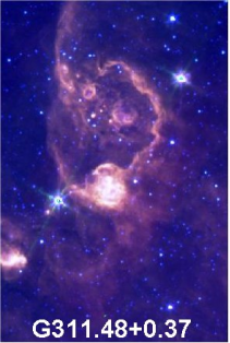
For example, Fig. 20 (in §8) shows compact cores, a large, faint, partial shell, many separate, small, internal shells, filaments, and even diffuse emission. The highest surface brightness pixels occur in the very bright central core. The second highest levels are found in the small, complete rings north of the bright core, and the third in the long, curving filament that emerges to the north-west from the core, looping around to the north and almost reaching the brighter of the two small rings inside the large, faint oval shell. Hence, “Cs” is our designation. Tertiary characteristics are not given for simplicity so the secondary code describes whichever aspect is brightest after the primary. Had we used a third descriptor then G311.48+0.37 would have been “Csf”. Parentheses around a primary code imply that it is not definite that the MIR source is the counterpart of the radio object.

Table 1. The sample of Hii regions with radio and MIR morphologies, integrated MIR and radio flux ratios, and 8.0-$\mu$m fluxes Source Size Radio IRAC IRAC/ MSX/ IRAC/ IRAC Fig. (arcmin) morph. morph. MSX MOST MOST mJy G310.63–0.43 $<$1 C Cf 1.64$\pm$0.20 23$\pm$1 37$\pm$5 17600 G310.68–0.44 $<$1 C Cf 1.49$\pm$0.20 23$\pm$1 34$\pm$4 13800 G310.69–0.31 $<$1 C UC 1.16$\pm$0.15 5.0$\pm$0.2 6$\pm$1 5100 G310.80–0.38 7$\times$6 S Dc … 8$\pm$1 … … G310.89+0.01 $<$1 C Cs 0.93$\pm$0.12 37$\pm$2 34$\pm$4 7200 18 G310.90–0.38 $<$1 C Ch 1.10$\pm$0.15 11$\pm$1 12$\pm$1 9600 G310.99+0.42 5$\times$7 S S 2.02$\pm$0.29 120$\pm$10 250$\pm$30 363000 23 G311.12–0.28 7$\times$8 S Dc 0.98$\pm$0.13 15$\pm$1 15$\pm$2 50000 G311.20+0.75 6$\times$15 S Cf 3.63$\pm$0.63 46$\pm$6 170$\pm$20 325000 G311.29–0.02 15$\times$14 F Dc 6.27$\pm$0.78 40$\pm$4 250$\pm$40 831000 G311.30+0.90 8$\times$4 S D 1.14$\pm$0.15 72$\pm$2 82$\pm$10 64000 G311.37+0.79 8$\times$24 F Dc 1.73$\pm$0.27 87$\pm$9 150$\pm$20 298000 G311.42+0.60 $<$1 C Cs 1.83$\pm$0.23 74$\pm$5 140$\pm$20 25000 16 G311.48+0.37 5$\times$8 S Cs 1.19$\pm$0.16 24$\pm$1 29$\pm$4 129000 20 G311.50–0.48 8$\times$8 S D 2.16$\pm$0.29 15$\pm$0.5 32$\pm$4 111000 24 G311.53–0.13 2$\times$9 F Df 1.93$\pm$0.26 20$\pm$1 38$\pm$5 21000 G311.59–0.59 $<$1 C Cf 1.61$\pm$0.20 17$\pm$1 28$\pm$3 7600 17 G311.62–0.60 11$\times$12 S Dc 1.31$\pm$0.18 66$\pm$7 86$\pm$10 189000 G311.63+0.29 $<$1 C Cm 2.63$\pm$0.32 13$\pm$1 34$\pm$4 32800 G311.64+0.97 35$\times$30^a F F 1.70$\pm$0.23 48$\pm$5 82$\pm$10 43600 G311.70+0.31 3$\times$2 F C(§9) 1.71$\pm$0.32 27$\pm$5 46$\pm$7 4800 G311.87–0.24 $<$1 C Ch 1.61$\pm$0.21 18$\pm$1 29$\pm$3 9000 G311.90+0.08 6$\times$6 S Cf 2.30$\pm$0.31 26$\pm$2 59$\pm$7 340000 G311.93+0.21 6$\times$5 S Cf 1.64$\pm$0.22 25$\pm$1 42$\pm$5 274000 G311.97–0.05 6$\times$4 B Dc 2.30$\pm$0.46 33$\pm$6 75$\pm$11 65700 G312.11+0.31 $<$1 C Cs 1.47$\pm$0.20 28$\pm$1 41$\pm$5 42400 G312.36–0.04 $<$1 C Df 1.13$\pm$0.19 24$\pm$3 28$\pm$3 13200 G312.45+0.08 60$\times$90 F F 1.46$\pm$0.35 800$\pm$200 1200$\pm$230 9460000 26 G312.50+0.32 5$\times$10 F D 1.56$\pm$0.24 53$\pm$6 83$\pm$10 68500 G312.58+0.40 8$\times$7 B Cm 1.85$\pm$0.24 37$\pm$2 69$\pm$9 57000 G312.59+0.22 3$\times$4 B Df 2.34$\pm$0.40 29$\pm$4 68$\pm$10 45800 G312.60+0.05 $<$1 C Ch 2.46$\pm$0.31 48$\pm$2 120$\pm$15 15700 19 G312.67–0.12 3$\times$1 B S 1.46$\pm$0.24 57$\pm$8 83$\pm$12 12300 22 G312.68+0.04 3$\times$4 Ci Si 2.39$\pm$0.35 31$\pm$3 75$\pm$10 38300 21 G312.71+0.02 3$\times$3 Ci Si 1.05$\pm$0.15 33$\pm$4 35$\pm$5 18000 18 G312.72–0.14 $<$1 C (S) 0.98$\pm$0.13 83$\pm$2 82$\pm$10 15900 G312.77+0.06 $<$1 C Ch 1.94$\pm$0.25 250$\pm$20 500$\pm$60 28600 15 G312.93–0.09W 8$\times$9 S D 1.75$\pm$0.23 59$\pm$4 100$\pm$15 88000 G312.95–0.44 5$\times$4 S Si 1.06$\pm$0.18 40$\pm$5 43$\pm$5 60900 G313.07+0.32 5$\times$4 S Df 1.24$\pm$0.26 64$\pm$15 79$\pm$15 30000 25 G313.32+0.05 8$\times$3 F D 0.98$\pm$0.13 30$\pm$2 21$\pm$3 60600 G313.37+0.02 9$\times$3 S Dc 1.27$\pm$0.17 74$\pm$1 94$\pm$11 37700 G313.46+0.19 $<$1 C Ch 1.79$\pm$0.24 16$\pm$1 28$\pm$3 22000

Footnote: ^a We used the maximum bright area of 6$\times$14 arcmin of this region that was covered by GLIMPSE

4 COMPARISON OF SST AND MSX INTEGRATED FLUXES

CG used matched-resolution MSX and radio images to derive their MIR-to-radio ratios. The Galactic Plane is particularly rich in both local and more distant structures which emit in the PAH bands. Accurate photometry of extended sources in the presence of this clutter requires special care. This affects MSX 8.3-$\mu$m measurements and potentially three IRAC bands (3.6, 5.8, and 8.0 $\mu$m) containing PAH fluorescent features at 3.3, 6.2, 7.7, and 8.7 $\mu$m. The coarseness of the low-resolution MSX images could have caused us to discriminate poorly between faint MIR emission and sky background. For example, we might have sampled inappropriately bright regions to assess the sky emission, particularly if we now wish to seek faint outer haloes. Therefore, we have twice remeasured all regions in the images with 46^′′ resolution (36^′′ pixels), paying particular attention to the choice of local sky background and using more than a single local area to assess the variations in sky background whenever possible. We have repeated this same procedure on the 20^′′ resolution (6^′′ pixel) “high-resolution” MSX images, better to assess the detectable extent of the sources, and with the same considerations of the sky emission to be subtracted. In this paper, we use the average of these two sets of measurements to provide our best estimates of the 8.3-$\mu$m flux densities of these extended regions. We have quantified the likely uncertainties in these integrals using the dispersions of the several sets of sky-subtracted measurements for each source. The average fractional uncertainty in these 8.3-$\mu$m areal integrations was found to be 6 percent.

For the IRAC fluxes in all four bands we have likewise sought to include all IR emission apparently associated with the radio sources in our spatial integrals, and to identify background that is well outside the radio sources. Unlike the MSX images, we have worked from GLIMPSE “residual images”. These are 1.1^∘$\times 0.8^{\circ}$ images with 0.6^′′ pixels from which all GLIMPSE point sources have been removed. The residual images are ideal for enhancing the recognition of diffuse nebulosity in regions of high point source density. They enable far more reliable photometry of such emission than can be obtained in the presence of the many point sources in the field. The residual images reflect the subtraction by our adaptation of DAOPHOT for GLIMPSE of all sources detected down to 2$\sigma$, deeper than our publically released Catalog and Archive point source lists that extend down only to 10 and 5 sigma, respectively. Thus there are faint 2$-$3-$\sigma$ points that are subtracted from the residual images that are not listed anywhere in our lists. Residual images still contain sources not extracted by DAOPHOT, such as saturated sources and sources that peak beyond the non-linearity limit for each band. These objects were individually integrated and their flux densities subtracted from the integrals over the relevant regions. (Fig. 27 illustrates a residual image.) PSF-subtracted residual artefacts consist of both negative and positive portions, often with a near-zero net integral. These usually have very little effect on integrations of diffuse emission but they can make contributions of order 1$-$10 percent to small areas of integrated sky background. Therefore, we removed all such artefacts that lay within regions we took to assess the sky, and likewise subtracted the brightest recognizable artefacts lying within the boundaries of Hii regions.

4.1 A statistical approach to removing MSX point sources

To compare the truly diffuse component of emission for an Hii region measured from MSX imagery with that assessed from the corresponding IRAC residual image one must subtract the contribution made to the total MSX brightness by point sources. This is required to avoid biasing the direct ratio of IRAC and MSX brightnesses by the inclusion of faint point sources in the MSX images. We emphasize that, were this the case, the ratio obtained would be lower than the true value because the MSX brightness would have been overestimated. Ideally one should remove the identical point sources from MSX images as from the IRAC images but these are roughly 1000$\times$ deeper than MSX so the vast bulk of GLIMPSE point sources were completely undetected, and undetectable, by MSX.

The majority of GLIMPSE sources are normal stars that appear faintest to IRAC in the 8.0-$\mu$m band, and were undetected by MSX. Any MSX point sources in the Hii regions that were discernible to the eye (i.e. at least 3$\sigma$) were integrated separately and their fluxes removed from that of the region. The median number of point sources subtracted per region was four. For a region with up to four point sources this approach was the simplest option and it was applied to more than half of our sample of Hii regions. For the seventeen regions having five or more point sources we queried the latest MSX Point Source Catalog (ver.2.3) using the “Gator” search tool at the Infrared Processing and Analysis Center (IPAC) and summed the flux densities of the resulting table of sources with detections within the specified area.

In future investigations we would like to be able to remove the influences of point sources of MSX on wide area (tens to hundreds of square degrees) integrated fluxes as accurately as possible, including objects with signal-to-noise values of less than $3-5\sigma$. Such weak objects cannot be drawn from the MSX Reject Source Catalog due to the heterogeneity of this Catalog (that can compromise the validity of the sources themselves) and to the effects of Malmquist bias (that overestimate the flux densities for valid weak sources). Therefore, we have used the present paper as a formal test of a statistical method that relies on the use of the “SKY” model originally presented by Wainscoat et al. (1992) but with considerably expanded capabilities. Not only does the model reliably predict the LogN-LogS distribution of bright and faint point sources in arbitrary directions, in any user-supplied system band from the far-ultraviolet to the MIR, it is also capable of summing up the smeared surface brightness due to unresolved and unrecognized point sources in any given area. This “Total Surface Brightness” mode was first described by Cohen (1993a), was applied to COBE/DIRBE diffuse sky maps (Cohen 1993b), and has undergone testing since then in a variety of different spectral regimes (e.g. Cohen 2000). Only one region in our sample contained so many MSX 8.3-um point sources that one could not remove them manually and one might not want to do so even by listing all sources in the MSX PSC2.3 and the Reject Source Catalog because of the likely impact of Malmquist bias on the resulting summation of flux. This area is G312.45+0.08, a 1.5${}^{\circ}\times$1^∘ area containing the largest diffuse structures in this field and straddling the Galactic plane. It is, therefore, well-chosen in terms of sampling the highest surface densities of point sources as well as containing much clutter in the form of bright nebulous filaments. The newest version of the SKY model successfully predicts GLIMPSE IRAC source counts by including the warp of the disk and was used for the calculations below.

The brightest and faintest stars in this field have magnitudes at 8.3 $\mu$m of $-$0.06 and 7.05, respectively (62 Jy and 88 mJy). The statistical assessment of star counts in this 1.5 deg² area came from the computation that the total brightness of all point sources within these limits in the MSX 8.3-$\mu$m band amounts to 5.44$\pm$0.22$\times$10^-11 W m^-2deg^-2. Dividing by the MSX bandwidth and scaling by 1.5 for the total area observed yields 582$\pm$23 Jy. We have tested these SKY predictions by directly finding all 8.3-$\mu$m point sources in the MSX PSC2.3 that lie within the rectangle defined by G312.45+0.08, by a corresponding J2000 Equatorial polygon search using the IPAC Gator tool. Eliminating all sources that were undetected (i.e. have quality flag of 0 or 1) results in a total of 693 point sources whose accumulated flux density is 542$\pm$24 Jy, statistically the same ($\sim 1\sigma$) as SKY predicts. We conclude that SKY is a viable tool for assessing total surface brightness due to point sources in any region and we have utilized its capability in this paper to ensure that effectively the same set of point sources has been removed from the MSX images as from the IRAC residual images.

SKY predicts more flux than that observed which is as expected because the MSX Point Source Catalog may not be complete to 7.05 magnitude because of the clutter of the interstellar medium (ISM) due to PAH emission. Therefore, we also need a SKY calculation for MSX that mimics the DAOPHOT extraction process that generates the IRAC residual images, by removing all point sources to the 2$\sigma$ level, corresponding to 8.0 magnitude. That calculation yields 625$\pm$26 Jy for the MSX point sources that would have been subtracted to the same brightness level as in our IRAC residual images at 8.0 $\mu$m. The observed sum of diffuse and point sources in the box integrated is 7100 Jy. Therefore, point sources contribute only 9 percent of the integrated emission and the diffuse component is 6480 Jy in this very large area. For a more typical diffuse region in our sample, with an area of $\sim$90 arcmin², the point source contribution subtracted from the total integrated light at 8.3 $\mu$m is $\sim$6.5 Jy, or 4 percent. Thirteen of the fifteen compact and ultracompact sources have three or fewer recognizable MSX point sources to magnitude 7.0, and their contribution is between 0.3 and 2 percent of the dominating emission of the ionized zone itself. For the line-of-sight to the centre of each Hii region we ran the SKY model to compute the additional contribution made by point sources, fainter than the limit to which we could recognize sources in the MSX image, and extending down to magnitude 8.0 at 8.3 $\mu$ to match the sources already removed from the coresponding IRAC residual image. The difference between assessing the MSX point source light extrapolated by SKY to magnitude 8.0 and removing identified sources to magnitude 7.0 is only about 7 percent of the contribution of point sources identified to magnitude 7.0. Therefore, except for extremely large diffuse areas such as G312.45+0.08, in individual Hii regions the removal of recognizable MSX point sources accounts for about $1-4$ percent of the total measured diffuse emission. The model extrapolations, to match the depth of removal of point sources in the IRAC residual maps, imply the subtraction of only about an extra 1 percent or less of the diffuse emission, well below the errors in the MIR integrated photometry of the same regions.

We now summarize the corrections applied to the total integrated emission of regions for the contribution of point sources. The IRAC images from which we start the analysis are already point-source subtracted to a depth of 8.0 magnitude at 8.0 $\mu$m. We further remove artefacts by hand that correspond to slight mismatches between our PSFs and real point sources. To subtract as closely as possible the same sources from MSX images as were removed in constructing the IRAC residual images ,we used a combination of techniques as follows, according to the character and apparent size of the Hii region. For compact and ultracompact objects we measured fluxes of all recognizable point sources if fewer than five were seen in the image, and subtracted their total flux from the measured diffuse emission. For regions containing five or more point sources we extracted those using Gator and summed their fluxes. We extended every Hii region below the local 8.3-$\mu$m magnitude limit for unambiguous identification in our MSX images by using the SKY-predicted total of surface brightness due to faint point sources in that direction. This contribution was subtracted from the photometry for each target region. We believe that this combination of techniques applied to the MSX images to account for point source removal is the best that can currently be achieved to match the depth of the IRAC residual images. If any starlight has been missed by the removal of actual sources and our extrapolation using SKY, it should be negligible compared with the diffuse flux attributable to any given Hii region.

No statistical model of the sky, however physically realistic (as is SKY), can predict the occurrence of individual young star clusters either along the line-of-sight or within Hii regions. Indeed, objects in the bright cores of HII regions are observed on top of bright nebular emission and will not appear pointlike. Thus DAOPHOT will not identify them as point sources nor will they be removed from IRAC residual images. One might be concerned that such clusters would be treated differently by our handling of point source removal from MSX and IRAC images. However, our field contains no giant Hii regions nor complexes with multiple star-forming centers, commonly the sites of embedded clusters. None of our bright-cored regions, nor the more diffuse, open structured regions reveals any projected or apparent internal clusters to IRAC. This is largely because of the use of this field to demonstrate the capabilities of the MOST survey by WCL. It is also a consequence of CG’s choice to carry out their MIR-radio study, intended to focus on the ISM, and on interactions between the medium and individually dominant stars, in this same field. Our analyses of MSX images, therefore, suffer from no bias with respect to those of IRAC that is caused by unresolved star clusters.

There are no low-resolution GLIMPSE images like the ones we used for MSX that offer quasi-independent photometry. Based on a series of tests carried out on diverse Hii regions of the reproducibility of our measured sky-subtracted fluxes we have assigned

Figure 1: Matched-area images of G310.99+0.42. Left: MSX, 8.3 $\mu$m. Right: IRAC, 8.0 $\mu$m.

Figure 2: Matched-area images of G312.60+0.50. Left: MSX, 8.3 $\mu$m. Right: IRAC, 8.0 $\mu$m.

a 12 percent uncertainty to the IRAC spatial flux integrals. The associated tests involved varying the choice of local areas from which to assess the diffuse sky background.

4.2 Direct comparison of MSX and IRAC images

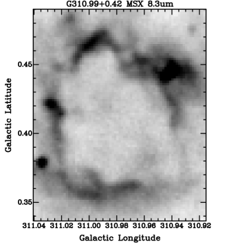
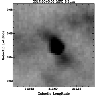
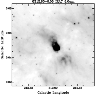
To illustrate the similarities and differences between MSX and IRAC images of the same regions we present grey-scale images of two fields (Figs. 1 and 2). MSX images of Hii regions are generally sparsely populated by point sources. We have chosen G310.99+0.42 because it shows a rather typical situation: many point sources but almost all of them undetected by MSX. The few that MSX saw are mostly avoidable by careful selection of the bounding rectangle for integration, or are readily isolated and integrated separately (which we generally did). By contrast we also show a compact region apparently immersed in diffuse emission: G312.60+0.50, where SST shows a wealth of point sources but MSX does not.

Figure 3: Log-log plot of IRAC 8.0-$\mu$m vs. MSX 8.3-$\mu$m flux densities distinguishing Hii regions of four different characters: ultracompact and compact; shells; diffuse; and filamentary. The key indicates the symbol associated with the radio character of each object, based on our new MIR morphology. The two lines represent the regression relationships for 42 regions (dashed) and for the subsample of the 25 apparently smallest and densest sources (solid).

The fifth column in Table 1 gives the ratios of IRAC 8.0-$\mu$m to MSX 8.3-$\mu$m integrated fluxes, with their statistical uncertainties. Fig. 3 presents the regression of these MIR fluxes, with errors in both variables. Symbols distinguish between Hii regions of four different characters as indicated in the key (ultracompact and compact; shells; diffuse; and filamentary.) The two lines differentiate between the regressions for the total sample of 42 regions available with the SST (dashed) and for the subsample of the 25 regions with the best defined morphologies (solid); i.e. for all objects that we categorize as ultracompact, compact, or shells. The unusual object, G311.70+0.31 (§9), was included with these compact sources because of its small apparent size and well-defined structure. This subsample lacks all the diffuse and filamentary regions.

Table 2 summarizes these results for each ratio of attributes by subgroup, giving the median, standard error of the median, size of the subsample, slope and offset with $1\sigma$ errors for the regression between logarithmic quantities, and the Pearson correlation coefficient between the two sets of MIR flux densities. The table is essentially divided between those regions that are well-defined and/or dense, those with complete or partial shell-like structures, and those consisting primarily of diffuse material, tenuous filaments, or bubbles. Specifically the categories of Hii regions for which results are presented in Table 2 are: ultracompact and compact combined (“U/C”); shells (“S”); ultracompact, compact and shells combined (“U/C/S”); diffuse and filamentary combined (we have only two filamentary regions) (“D/F”); and the entire sample. Further conbinations of morphological subcategories reveals no meaningful differences in the ratio IRAC/MSX with respect to the character of the region.

The regression for the entire sample has a slope of 1.07$\pm$0.03 (1.00$-$1.14, $\pm 3\sigma$ range), while that for the 25 densest and apparently smallest objects has a slope of 1.05$\pm$0.03 (0.98$-$1.13, $\pm 3\sigma$ range). There is no statistically significant difference between the two correlations. Both are consistent with linear proportionality between SST and MSX 8-$\mu$m fluxes, have good correlation coefficients, and span three and a half orders of magnitude in observed dynamic range of MIR flux.

We have also carried out an independent analysis of the data offered in this paper using the types assigned by WCL (cometary, compact, classical, “Hii”, “thermal”, filamentary (including bubbles), low-density). These are somewhat informal designations drawn from heterogeneous literature and there are no significant distinctions in terms of the ratio of IRAC to MSX 8-$\mu$m flux densities even among WCL’s types.

The entire sample available to define the ratio of IRAC/MSX near 8$\mu$m consists of 42 regions and yields a median of about 1.6. There are no significant differences between this and any subsample of regions. The similarity of the ratios in physically very different sources such as diffuse and compact Hii regions confirms the reality of this effect and marks it as a problem with the IRAC calibration. Our best quantitative estimate of the effect comes from an independent median analysis of the 25 smallest and densest regions: 1.55$\pm$0.15. This is the empirical ratio of IRAC 8.0-$\mu$m/MSX 8.3-$\mu$m found for these regions.

Table 2. Analysis of ratios of IRAC 8.0-$\mu$m/MSX 8.3$\mu$m, MSX/MOST, and IRAC/MOST fluxes and sample sizes (in parentheses), and log-log regressions. IRAC/MSX MSX/MOST IRAC/MOST Group median$\pm$ slope$\pm$ offset$\pm$ correl. median$\pm$ slope$\pm$ offset$\pm$ correl. median$\pm$ slope$\pm$ offset$\pm$ correl. sem(no.) $\sigma$ $\sigma$ coeff. sem(no.) $\sigma$ $\sigma$ coeff. sem(no.) $\sigma$ $\sigma$ coeff. U/C 1.6$\pm$0.2(19) 1.07$\pm$0.03 $-$0.1$\pm$0.1 0.97 25$\pm$5(18) 1.00$\pm$0.02 1.3$\pm$0.1 0.88 36$\pm$13(18) 0.98$\pm$0.03 1.6$\pm$0.1 0.82 S 1.5$\pm$0.3(6) 1.14$\pm$0.07 $-$0.5$\pm$0.3 0.96 45$\pm$20(6) 1.11$\pm$0.05 1.5$\pm$0.1 0.87 78$\pm$24(6) 1.21$\pm$0.07 1.3$\pm$0.2 0.84 U/C/S 1.6$\pm$0.2(25) 1.05$\pm$0.03 $-$0.1$\pm$0.1 0.97 27$\pm$13(24) 0.99$\pm$0.01 1.4$\pm$0.1 0.83 41$\pm$14(24) 0.93$\pm$0.02 1.8$\pm$0.1 0.79 D/F 1.6$\pm$0.4(17) 1.11$\pm$0.04 $-$0.3$\pm$0.2 0.96 44$\pm$18(18) 0.77$\pm$0.03 2.3$\pm$0.1 0.72 82$\pm$25(17) 1.29$\pm$0.04 0.9$\pm$0.1 0.80 All 1.6$\pm$0.2(42) 1.07$\pm$0.03 $-$0.1$\pm$0.1 0.97 33$\pm$18(43) 0.93$\pm$0.02 1.6$\pm$0.1 0.77 63$\pm$26(42) 1.03$\pm$0.02 1.7$\pm$0.1 0.77

5 MIR spectra of Hii regions: the diffuse calibration of IRAC at 8.0 microns

In addition to the SSC’s formal study of aperture correction factors, there is an analysis of the IRAC extended source calibration by Jarrett (2006), now an official SSC page, based on a sample of twelve elliptical galaxies whose observed light distributions have been modeled. That work finds a flux correction factor that varies from 0.78 to 0.74 at 8.0 $\mu$m, with a probable uncertainty of 10 percent. This factor is the inverse of our IRAC/MSX ratio and, therefore, implies ratios of 1.28$-$1.35, adopting MSX as the fiducial. That the ratios of IRAC/MSX exceed unity is believed to be due to scattering of light internal to the IRAC detector arrays, and it is a particular problem in the Si:As arrays (the 5.8 and 8.0-$\mu$m bands). The origin of the scattered light is thought to be in the epoxy layer between the detector and multiplexer. The glue has a strong spectral response, peaking in the 5$-$6-$\mu$m region (Hora et al. 2004a).

Figure 4: Comparison of the in-band portions of the relative spectral response curves for MSX’s 8.3-$\mu$m (solid) and IRAC’s 8.0-$\mu$m bands (dash-dot).

Not all of this excess is attributable to light scattering, however. The IRAC 8.0-$\mu$m band has a very different relative response curve from the broader, somewhat longer, MSX 8.3-$\mu$m band (Fig. 4), and the effects of this difference when integrating over the spectra of Hii regions must be treated. This we have done by three different methods. First we used the 2$-$35-$\mu$m template for Hii regions, one of 87 such templates developed by Cohen (1993) to give the SKY model of the point source sky its capability to predict source counts for arbitrary IR bands. This normalized template spectrum was constructed as the average of the observed spectra of 10 bright, rather compact (measured with beams between 3.4^′′ and 30^′′ in diameter) Hii regions. Within these IRAC and MSX bands the dominant spectral features from the cores ($\sim$1 arcmin in diameter) of Hii regions are (ranked by strength): a strong dust continuum, very deep 10-$\mu$m silicate absorption; deep 6.0-$\mu$m water absorption; PAH emission at 7.7 $\mu$m; and, sometimes, weak fine structure lines (Willner et al. 1982). Integrating the two spaceborne bands over this ($\lambda$,F_λ) spectrum yields in-band fluxes of 1.75$\times 10^{-15}$ W cm^-2 (SST) and 1.90$\times 10^{-15}$ W cm^-2 (MSX). Dividing by the corresponding bandwidths ($1.146\times 10^{13}$ and $1.402\times 10^{13}$ Hz) gives 0.0153 and 0.0135 Jy, respectively. Consequently, in an optically perfect instrument, one would expect IRAC/MSX = 1.12$\pm$0.03. Away from the embedded central ionizing source, the spectrum of extended emission from the PDR is still that of cool dust, overlaid by spatially extended silicate absorption, with diffuse PAH emission, and fine structure lines, even in large regions such as M17 (e.g. Kassis et al. 2002). Therefore, Cohen’s template is still relevant because the bulk of the energy is emitted from the hot central core of an extended Hii region.

The second method seeks to define the best average spectrum of the Hii regions in the field under study here, rather than relying on an average composed of the most famous and brightest compact regions. The Hii region template is a combination of ground-based

Figure 5: Calibrated LRS spectra for 11 Hii regions in the field. Error bars are $\pm 1\sigma$ at each wavelength. Our own, and WCL’s (in parentheses), morphological types are given in each separate plot.

and airborne spectra, bridging gaps using data from the IRAS Low Resolution Spectrometer (LRS: Wildeman, Beintema & Wesselius 1983). LRS coverage is from 7.7$-$22.7 $\mu$m and each spectrum consists of two sections, blue and red, whose effective apertures were $6^{\prime}\times 5^{\prime}$ and $6^{\prime}\times 7.5^{\prime}$, respectively. For substantially extended sources the convolution of spatial structure and wavelength in these large apertures requires a complex extraction process. Sources smaller than 15^′′ are not affected by the convolution (Assendorp et al. 1995). However, many Hii region spectra were published in the Atlas of LRS spectra (Olnon et al. 1986), based on a much simpler extraction method. This approach yielded perfectly adequate spectra (benchmarked by Cohen (1993) against ground-based and airborne spectra in the construction of SKY’s 87 templates) because most of the bright infrared emission of Hii regions arises in volumes of small apparent size. The complete Dutch LRS database comprised 171,000 LRS spectra, derived by using the same software as Olnon et al. (1986), and we have sought spectra for all the Hii regions in the l = 312^∘ field in this database. We incorporate the recalibration of LRS spectral shape provided by Cohen et al. (1992a), and normalize the resulting spectra to the absolute 12-$\mu$m flux densities (scaled by the factor of 0.961 described by Cohen et al. (1996: their Table 6) as applicable to IRAS 12-$\mu$m flux densities of both the Point Source Catalog (PSC) and the Faint Source Survey). When available we used the PSC flux density; otherwise that from the Faint Source Reject catalog. We found 93 LRS spectra for 32 regions, and were able to extract useful averages for 11 of these regions.

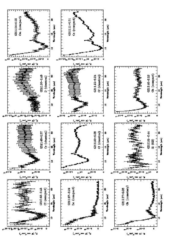
Fig. 5 presents the 11 averaged, calibrated spectra. Nine of these are somewhat similarly shaped; two others are quite distinct because of their blueness: G311.87$-$0.24 (Dc) and the cometary G312.77+0.06 (Ch). Each individual spectrum is plotted in F_λ, and carries the source designation, and both our type and that assigned by WCL. Error bars are $\pm 1\sigma$ at each wavelength. Quality varies from source to source although the characteristic deep 10-$\mu$m silicate absorption is seen in almost all the objects. Deep silicate absorptions might indicate the presence of accretion disks that are viewed edge-on, but the frequency of these in Hii regions suggests that, in most regions, these absorptions occur because of deep embedding of the exciting stars in more spheroidal dusty envelopes.

We created the average of the nine most similar spectra by inverse-variance weighting each spectrum (peak normalized to unity) based on the wavelength-dependent uncertainties that our reduction code produces (Cohen et al. 1992a). Fig. 6 compares this average LRS spectrum with the complete 2$-$35-$\mu$m spectral template from the SKY model. The agreement between the two normalized spectra is very good between the LRS cut-on (7.7 $\mu$m) and the long wave limits of the bandpasses of the relevant MSX (e.g., 1 percent transmission at 11.08 $\mu$m) and SST filters (1 percent transmission at 9.63 $\mu$m). In the MIR, ionic lines do not contribute greatly to the content of the SST and MSX bands.

We have constructed a hybrid spectrum by taking the data below 7.67 $\mu$m from the SKY template, and the average of the nine LRS spectra for our actual Hii regions beyond this wavelength. We integrated the MSX 8.3-$\mu$m and SST 8.0-$\mu$m relative spectral response curves over this spectrum, resulting in a ratio of the two instruments’ flux densities of IRAC/MSX = 1.17$\pm$0.03.

For the truly diffuse ISM the same calculations can be performed using spectra taken in the large-aperture ($8\times 8$ arcmin) near-infrared and MIR spectrometers of the Infrared Telescope in Space (IRTS: Onaka 2003, Sakon et al. 2004). We have assembled a spectrum from 1.4$-$11.67 $\mu$m based on the IRTS and for this the ratio of integrated flux densities, IRAC/MSX, is 1.15$\pm$0.06. The IRTS spectrometers were calibrated (Tanabe et al. 1997, Onaka et al. 2003, Murakami et al. 2004) with the identical basis to that embracing the IRAS LRS, MSX, and the SST so that integrations over this diffuse spectrum are directly comparable to those over the LRS and SKY template spectra. The same procedure can be applied to the ISOCAM CVF spectra of the ISM presented by Flagey et al. (2006). We computed the ratio IRAC/MSX for their spectrum with the most relevant longitude, the 299.7^∘ field, and obtained 1.11. However, the traceability of the CAM CVF flux calibration is not identical to that of the MSX and SST and we assign this value twice the error of that derived from the IRTS spectrum. Consequently, whether we observe the most compact of cores, spatially extended MIR emission associated with Hii regions, or the ISM at large, we obtain a robust result for the measured ratio of IRAC/MSX near 8 $\mu$m with the empirical spectra of diffuse Hii regions, namely 1.14$\pm$0.02 (by inverse-variance weighting of our four values).

The actual ratio determined for IRAC/MSX is 1.55, of which the factor of 1.14 is attributable solely to the different in-band fluxes measured by these two bands for the MIR spectrum of Hii regions. Internal scattering in IRAC’s 8.0-$\mu$m detector, therefore, contributes the additional factor of 1.36$\pm$0.13 to the ratio of IRAC 8.0-$\mu$m/MSX 8.3-$\mu$m based on our analysis of Hii regions. Expressed as the reciprocal quantity (the aperture or flux correction factor of SSC and Jarrett (2006)) our analysis is equivalent to 0.74$\pm$0.07. For comparison, the average correction factor and a conservative uncertainty of the elliptical galaxies at 8.0 $\mu$m is 0.74$\pm$0.07, while Reach et al. (2005) recommend 0.737 (no uncertainty specified) at 8.0 $\mu$m. Therefore, our independent analysis of the diffuse flux correction of IRAC at 8.0 $\mu$m based on Hii regions is consistent with two separate analyses based either on the performance of the instrument, or on models of the IR light distributions of elliptical galaxies.

In the low surface brightness regime, the minimum detectable diffuse emission in this field has an intensity at 8.3 $\mu$m of about 1.0$\times 10^{-6}$ W m^-2 sr^-1. At the same location the IRAC 8.0-$\mu$m level is 1.4$\times 10^{-6}$ W m^-2 sr^-1, consistent with the same factor for IRAC/MSX as measured for the bright Hii regions.

Figure 6: Comparison between the SKY template for generic Hii regions (solid line) and the average of 9 regions in this field (filled squares with$\pm 1\sigma$ error bars). Open rectangles show the locations of the normalized median SED for the regions (§6).

6 Spectral energy distributions

We have taken the spatially integrated flux densities (in Jy) from the images and multiplied by the bandwidths (in Hz) to generate in-band fluxes. These we converted to Vega-based magnitudes and, subsequently, into flux densities expressed in F_λ (in W cm^-2 $\mu$m^-1, after dividing by the bandwidths in $\mu$m. Table 3 presents the absolute calibration for IRAC based upon the newest released relative spectral response curves (July 2004) and the absolute Vega spectrum used to define zero magnitude (Cohen et al. 1992b) for IRAC and absolutely validated to 1.1 percent by Price et al. (2004). The assumed uncertainty on the response curves is 5 percent, independent of wavelength.

Table 3. IRAC zero magnitude absolute attributes with isophotal quantities and uncertainties below Filter Bandwidth In-Band F_λ(iso) $\lambda$(iso) Bandwdth F_ν(iso) $\nu$(iso)  $\mu$m W cm^-2 W cm^-2 $\mu$m^-1  $\mu$m Hz Jy Hz Error Error Error Error Error Error Error  $\mu$m % W cm^-2 $\mu$m^-1  $\mu$m Hz Jy Hz IRAC1 6.514E-01 4.277E-15 6.566E-15 3.550E+00 1.543E+13 2.771E+02 8.461E+13 3.890E-03 1.572E+00 1.104E-16 1.533E-02 6.375E+10 4.356E+00 7.047E+11 IRAC2 8.827E-01 2.342E-15 2.654E-15 4.494E+00 1.306E+13 1.794E+02 6.685E+13 5.707E-03 1.592E+00 4.560E-17 1.994E-02 5.834E+10 2.853E+00 5.657E+11 IRAC3 1.196E+00 1.237E-15 1.034E-15 5.725E+00 1.086E+13 1.139E+02 5.255E+13 8.376E-03 1.607E+00 1.813E-17 2.560E-02 5.182E+10 1.829E+00 4.381E+11 IRAC4 2.395E+00 7.230E-16 3.019E-16 7.837E+00 1.146E+13 6.310E+01 3.865E+13 1.663E-02 1.599E+00 5.263E-18 3.528E-02 5.242E+10 1.006E+00 3.172E+11

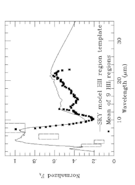
It is necessary, however, to apply corrections for what is known about the shortcomings of the diffuse calibration of this instrument. We have determined in this paper that the 8.0-$\mu$m calibration leads to fluxes too high by 36 percent. This can be compensated by applying an equivalent offset to the diffuse magnitude scale of +0.33. For IRAC’s three other bands we adopt the SSC analysis (footnote in §5) based on model template SEDs for elliptical galaxies. Averaging the “correction factors” derived from these galaxies indicates that corresponding offsets of +0.19, +0.09, +0.33 should be applied to measured diffuse magnitudes at 3.6 $\mu$m, 4.5 $\mu$m, and 5.8 $\mu$m, respectively. Table 4 incorporates these corrections for each band both to magnitudes and to the values of F_λ. The table summarizes integrated magnitudes of the sample of Hii regions giving the brightest and faintest magnitudes, and the medians with their standard errors. The dynamic range of the sample varies from a factor of 380 at 3.6 $\mu$m to 200 at 8.0 $\mu$m, and the difference between the median magnitudes at these two wavelengths (almost 5 mag) confirms the great redness of Hii regions. Every Hii region has its maximum IRAC F_λ in the 8.0 $\mu$m band. We normalized the quartet of F_λ values for every object by dividing by F_λ(8.0 $\mu$m), then took the median of each complete set of normalized values of F_λ(band)/F_λ(8.0 $\mu$m) where band = 3.6, 4.5, 5.8 $\mu$m. From the corrected magnitudes of the individual regions we have constructed Table 5, which presents the median values of the six colour indices between the four IRAC bands. Note that uncertainties are given for each offset based on the standard deviation of the average value of the colour’s correction factors for the nine galaxies. The errors in corrected colours are the RSS of the errors in the corresponding offsets and the standard errors of the medians. Those medians, with their standard errors, appear in col.(6) of Table 4. These normalized values represent a coarse SED over the IRAC range for Hii regions. Fig. 7 directly compares this SED with the template for the cores of bright Hii regions and the diffuse ISM template. The SED is represented by rectangles, horizontally as wide as each bandwidth and vertically as tall as $\pm$2 standard errors of the median. There is obviously much better agreement with diffuse emission than with the spectrum of a compact Hii region with its exciting star(s) and hot dust continuum.

Figure 7: Comparison of the median SED ($\pm$2 standard error rectangles) for thermal sources in this field with the diffuse ISM (solid line: IRTS, §4) and the SKY Hii region template spectrum (short dashed line).

Table 4. Vega-based magnitudes of the sample of Hii regions in the IRAC bands, and normalized F_λ SED. Band $\lambda$($\mu$m) Brightest Faintest Median$\pm$s.e.med. Median F_λ(band)/F(8.0 $\mu$m) 1 3.6 2.24 8.68 5.60$\pm$0.25 0.23$\pm$0.05 2 4.5 2.02 8.17 5.32$\pm$0.25 0.15$\pm$0.02 3 5.8 $-$0.58 5.21 2.71$\pm$0.25 0.66$\pm$0.02 4 8.0 $-$2.47 3.42 0.54$\pm$0.25 1.00$\pm$0.04

Table 5. Observed and corrected median Vega-based colours (in magnitudes) of Hii regions in the four IRAC bands Colour Observed Offset$\pm\sigma$ Corrected median median$\pm$s.e.med. $[3.6]-[4.5]$ 0.43 +0.11$\pm$0.02 0.53$\pm$0.06 $[3.6]-[5.8]$ 3.35 $-$0.13$\pm$0.03 3.22$\pm$0.10 $[3.6]-[8.0]$ 5.07 $-$0.13$\pm$0.03 4.94$\pm$0.10 $[4.5]-[5.8]$ 2.91 $-$0.24$\pm$0.03 2.67$\pm$0.07 $[4.5]-[8.0]$ 4.69 $-$0.28$\pm$0.03 4.41$\pm$0.08 $[5.8]-[8.0]$ 1.79 +0.00$\pm$0.04 1.79$\pm$0.05

Figures 8 and 9 present two interpretive colour-colour planes for IRAC bands showing the 87 categories of source in the version of the SKY model where each source is represented by a complete 2$-$35-$\mu$m spectrum (Cohen 1993). The caption to Fig. 8 details the symbols used for various populations. These colour-colour plots can be used for quick-look diagnostics of populations in random Galactic directions. Planetaries are represented by two large filled circles because young and evolved planetary nebulae occupy two distinct regions in IRAS colour-colour planes (Walker & Cohen 1988; Walker et al. 1989). Hora et al. (2004b) provide empirical IRAC colour-colour locations from their study of planetary nebulae with SST and their colours encompass the two larger circles predicted in Fig. 8.

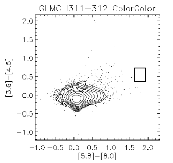
These figures show [3.6]-[4.5] vs. [5.8]-[8.0] and [4.5]-[5.8] vs. [3.6]-[8.0] diagrams. The large rectangles ($\pm$3 standard errors of the median) represent the zones in which diffuse Hii regions ought to fall based on the median corrected colours in col.(4) of Table 5. Correcting the observed colours using the offsets in col.(3) of Table 5 results in changes that are smaller than those that affect the magnitudes in any single band, and in no way alter the almost complete isolation of the diffuse Hii regions’ box in these plots. Only one of the 87 types of point source in these plots encroaches on the diffuse colour box (the cross, corresponding to one type of reflection nebula.) Fig. 10 displays the observed colour-colour plots for the GLIMPSE Catalog of point sources for the roughly 1 deg² field centred at l = 312.50^∘. Ultracompact sources would pass into the GLIMPSE Point Source Catalog for this field provided that their cores were not saturated in any of the four bands nor contained any other corrupted pixels within the core radius. However, their colours would mimic the bright, compact Hii region colours represented by the small filled circle in each of Figs. 8 and 9. It is interesting to note that there are three such pointlike sources observed with the colours of (ultra)compact Hii regions. There is only trivial contamination, by any of the 213563 observed point sources in the GLIMPSE Catalog for the 1 deg² region centred on 312.50^∘, of the corresponding colour-colour box that we have determined for diffuse Hii regions.

Figure 8: Diagnostic IRAC colour-colour plot ([3.6]-[4.5] vs. [5.8]-[8.0]) comprising 87 types of IR point source. Key: pluses - normal dwarfs, giants, supergiants; asterisks - AGB M stars; diamonds - AGB visible C stars; triangles - AGB deeply embedded IR C stars; squares - hyperluminous objects (these objects include deeply embedded OH/IR stars and early-type hypergiants (Cohen 1993; a small number are required to reproduce MIR source counts at low latitude: Wainscoat et al. (1992)); crosses - exotica (T Tau stars, reflection nebulae); larger filled circles - planetary nebulae; small filled circle - bright compact Hii regions. The reddening vector corresponding to an A_V of 10 mag is shown by the shaft of the arrow in the upper left corner. The large rectangle denotes the zone occupied by the extended Hii regions in this paper ($\pm$3 standard errors). Axis labels include magnitudes with “N” in their names to signify that new relative spectral response files from July 2004 were used for the IRAC bands.

Figure 9: As Fig. 8 but for [4.5]-[5.8] vs. [3.6]-[8.0].

Figure 10: Same axes as in Fig. 9 but based on the 213563 observed GLIMPSE point sources in the catalogue for this field. The densest regions of the plot are represented by contours rather than showing every source. The appropriate Hii region box shown in Fig. 8 also appears in this plot.

The overall dispersion in SEDs expressed by the IRAC colours is quite small, in part because of the rather limited contributions of emission lines in most Hii regions. The primary features in their MIR spectra are attributable to broad absorptions by silicates, ices, and organic materials. Cohen et al. (2005) considered the emission in the IRAC bands from ionized gas in a new planetary nebula found in GLIMPSE observations. Both free-free and hydrogen line emission were derived from the level of thermal radio emission but did not amount to more than a few percent in the IRAC bandpasses. Flagey et al. (2006) perform the same kind of estimates for the diffuse ISM, deriving no more than about a 12 percent contribution from recombination lines and free-free continuum even at the shorter IRAC wavelengths.

Fine structure lines are not bright in Hii regions as evidenced by their absence even in well-known compact sources (e.g. Willner et al. 1982). One can similarly gauge the minimal influence of emission lines in the LRS range through Fig. 5. Even for the IR-brighter sources in our field one sees only three 12.8-$\mu$m [NeII] lines and one object might show an 18.7-$\mu$m [SIII] line.

7 COMPARISON OF MIR AND RADIO FLUX DENSITIES

Fig. 11 compares the MSX 8.3-$\mu$m flux densities with those measured from MOST images (both in mJy). Fig. 12 similarly compares IRAC 8.0-$\mu$m flux densities with 843-MHz data. These two figures retain the different symbols to identify different types of thermal region. Table 2 summarizes the median analyses and regression lines for the subsamples of sources in terms of the ratios of MSX to MOST (centre of the table), and SST to MOST (right section of the table), flux densities.

There are meaningful correlations implying linear proportionality between both MSX and SST 8-$\mu$m fluxes and radio continuum fluxes. However, unlike the IRAC/MSX correlation, there are three issues which affect the MIR to radio flux ratios. One expects the MOST to lose flux substantially as the interferometer observes larger regions. The best model for the actual synthesized beam of the MOST incorporates an effective minimum spacing of about 70$\lambda$ (Hogan 1992) although this parameter varies between observations and may be dependent on meridian distance. Therefore, angular scales greater than about 30 arcmin are typically poorly detected. This certainly affects the largest structure in the field (the filamentary object, G312.45+0.08, MSX/MOST of 800) with a size greater than 1^∘. It might also overestimate MSX/MOST for the second largest source (the diffuse G311.37+0.79, MSX/MOST of 87), with a size of 24 arcmin, corresponding to the second largest Hii region in our whole sample. To assess the fraction of true radio continuum flux that has been measured for each specific region by the MOST would require detailed modeling based on the irregular structures of real sources, and on the u-v coverage obtained, like the simulations performed by Bock & Gaensler (2005). We can state only that MSX/MOST and IRAC/MOST ratios are invalid for G312.45+0.08 but we suggest that this phenomenon may also contribute to some of the other large ratios that are found in Table 2, particularly for diffuse regions.

The second concern is relevant to the single example of a cometary Hii region in our sample, G312.77+0.06. This appears anomalous in both Figs. 11 and 12 because it is quite compact yet also has a very large MIR/radio ratio. We believe this object is optically thick at 843 MHz, greatly diminishing the radio continuum flux density. This would be consistent with the extremely deep 10-$\mu$m silicate absorption whose optical depth, $\tau$(10 $\mu$m) $\approx$3, hence A_V$\approx$55 (Roche & Aitken 1984; Chiar & Tielens 2006), and the fact that this source has the most extreme LRS energy distribution in our sample in that it shows the deepest 18-$\mu$m silicate absorption too. The blueness of the spectrum implies an abundance of warm ($\geq$400 K) dust (rather than cool, i.e. $\leq$100 K) local to the embedded high-mass star. Consequently, this region’s exciting star is enormously embedded in dust, plausibly leading to local free-free absorption from the associated dense ionized gas. Therefore, we have chosen to exclude this region from any MIR/radio analysis of subsamples, reducing the ultracompact and compact Hii regions to 18 objects. However, samples designated as “All” in Table 2 include this cometary region.

Thirdly, our SST images have been culled of point sources (only their residuals after PSF subtraction remain) but we have no such products for MSX. Thus MSX fluxes within the radio source rectangles could potentially still include some faint point sources although efforts were made to remove their influence. Radio flux densities for big sources will suffer loss of signal because of resolving out structure as discussed above. Spitzer images are so sensitive to diffuse emission at low surface brightness levels that it could be necessary to seek uncontaminated sky at greater distances from the source than for MSX. This could lead to underestimated sky backgrounds, hence somewhat enlarged source fluxes for IRAC, and relatively reduced fluxes for MSX. Both effects could inflate the ratio of IRAC/MOST. Consequently, we chose matching sky regions for both IRAC and MSX to mitigate this problem. Our best estimate for these ratios will clearly come from the sample of the 18 most compact entities, excluding the cometary source. From this set we find MSX/MOST has a median of 25$\pm$5, in excellent accord with CG’s median of 24. The corresponding empirical ratio (i.e. with no flux correction factor applied) for SST is 36$\pm$13.

Figure 11: Log-log plot of MSX 8.3-$\mu$m vs. S(843 MHz) flux densities. Symbols and regression lines as in Fig. 3. The compact object near the left boundary in the plot whose filled symbol is also encircled represents the sole cometary region, G312.77+0.06, which has been excluded from the regression analyses of compact regions.

Figure 12: Log-log plot of IRAC 8.0-$\mu$m vs. S(843 MHz) flux densities. Symbols and regression lines as in Fig. 3.

Figures 13 and 14 seek correlations between MIR/radio flux densities and the type of Hii region, and its characteristic size, respectively. These figures are derived from the data presented in Table 2. It is sufficient to explore any trend with the ratio MSX/MOST, because we know SST and MSX fluxes are linearly correlated. A weak trend toward larger median ratios in less compact sources is suggested by Fig. 13 and explored in Fig. 14 in which we have attempted to quantify the size of the different morphology types, using the square root of the median of the areas in each category. For ultracompact and compact regions we have measured the full width at half maximum (above the surrounding sky) of the bright cores at 8.0 $\mu$m and have used this as the characteristic dimension for these objects. The median size of these 18 compact regions is 25$\pm$4 arcsec (standard error of the median), or 0.42 arcmin. The 15 regions whose ratio of MSX/MOST exceeds the median plus 3 standard errors of the median (a value of 40) consist of 3 compact, 2 shell, 7 diffuse, and 2 filamentary sources (excluding the self-absorbed G312.77+0.06). Each of these 3 compact regions also contains filaments, or shell structure or has a MIR halo. Therefore, this trend probably reflects the onset of the loss of radio signal with increasing apparent size.

It might instead indicate that compact regions other than G312.77+0.06 are dense enough to suffer self-absorption of free-free emission. Alternatively the trend might arise because the high density of dust in physically small sources leads to stronger MIR thermal continuum emission at the expense of fluorescent PAH bands. However, this would also increase the dust emission from small grains (PAH clusters with hundreds of carbon atoms) observed as a broad plateau of emission in the 8.0-$\mu$m IRAC band, underlying the 6.2, 7.7, and 8.7-$\mu$m bands. This would offset some of the lost PAH emission. Detailed modeling of specific regions is required to explore this alternative hypothesis, incorporating both the formation and destruction rates of PAHs and small grains, but this is beyond the scope of this paper.

There is significant scatter in Figs. 11 and 12 but one might have predicted even more than is observed because variations in excitation parameter and in 843-MHz optical depth from source to source would affect the radio spectral shape and turnover frequency. However, as CG concluded, most of the Hii regions in this field are not optically thick at 843 MHz; even the compact regions. The very fact that MOST detected so many regions argues that the old criterion, that below 1 GHz Hii regions are optically thick, is not sufficient. The general absence of optically thick regions at 843 MHz in the l=312^∘ field is also borne out by Figs. 13 and 14. The small MIR/radio ratios among compact objects implies there is little loss of 843-MHz signal. By comparison with the median of 25 for MSX/MOST for compact regions plotted in these figures, the cometary G312.77+0.06 has a ratio of 250, illustrating plausibly how these ratios would be affected by significant optical depth.

Figure 13: Medians and their standard errors for the ratio of MSX 8.3$\mu$m and MOST flux densities plotted sequentially for the four types of Hii region in the field. Our MIR morphologies are indicated under each median.

Figure 14: As Fig. 13 but the ratios are plotted against the logarithm of the median apparent size of objects in each morphological group.

Among the many Hii regions in this field is one object that would be defined as ultracompact, namely G310.69$-$0.31. The SST 8.0-$\mu$m image has all the characteristics of a minimally resolved bright source; a size between 1.5^′′ and 2^′′ (slightly in excess of the point spread function’s FWHM) and the hexagonal pattern of SST diffraction spikes. The residual image (with the suitably scaled PSF subtracted) shows a central hole at the core but has a saturated ring immediately around this hole to a radius of roughly 1^′′. Its ratio of IRAC/MSX is 1.16$\pm$0.08, exactly as predicted for a source with the SED of an Hii region that we have presented in Fig. 7. This result also confirms that IRAC photometry of a region dominated by a pointlike core (although we cannot exclude the existence of a very faint halo of emission) is essentially correctly assessed. Inspection of the Basic Calibrated Data images sugests that the object is at or near saturation at 8.0 $\mu$m, but not severely saturated. Therefore, we believe there is no major loss of flux in integrating its image and the IRAC/MSX ratio is credible. However, the source is too faint to have been detected by the LRS instrument. The ratios of both MSX/MOST (5) and IRAC/MOST (6) are the lowest of any source in Table 1, perhaps because dust competes more effectively for stellar UV photons than do PAHs.

8 MIR imagery of Hii regions

We present monochrome SST images of twelve objects that span the range of MIR morphologies of Hii regions in this field. These are chosen to highlight the structural MIR characteristics that can be associated with various radio types. Although the printed paper presents black and white renditions of the IRAC images, the electronic version shows them as 3-colour pictures in which 4.5-$\mu$m (blue), 5.8-$\mu$m (green), and 8.0-$\mu$m (red) images have been combined. Our reasons for this particular trio are as follows. Firstly, 3.6 $\mu$m shows too many stars and clutters the diffuse structure. MSX was often unable to provide the requisite confirmation of PAHs by the test of matching morphologies in its 8.3 and 12.1-um bands (both of which include PAH band emission) because the sensitivities of all its other bands were so much lower than that of the 8.3-$\mu$m band. By contrast, IRAC offers two sensitive bands capable of sampling PAH emission. In order to confirm the existence of PAHs, that are widely believed to be the dominant spectral features in diffuse Hii regions, we wished to see the same morphology emerge in IRAC’s 5.8 and 8.0-$\mu$m bands. One can also seek subtle changes in PAH populations through spatial variations in intensity ratios or, equivalently, in false colour across regions. For example, PAH emission from PDRs generally appears yellow or orange in our false-colour gallery because both 5.8 and 8.0-$\mu$m bands contain comparably strong fluorescent PAH emission features. With IRAC we still have a probe for H₂ lines through the 4.5-$\mu$m band too.

Although colour differences across a single Hii region have relative significance, note that variations between colour images of different regions do not necessarily indicate any spectral differences between the objects. Our intent was simply to offer colour images that would reveal the intrinsic structure of each region, setting the colour balance and contrast object by object, rather than aiming at an absolutely black “sky” for all sources, or a yellow level for PAHs that is constant for every source.

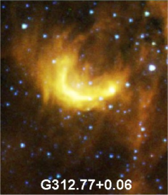
The MIR appearance of the cometary region in our sample (G312.77+0.06, Ch: Fig. 15) clearly resembles the canonical radio structure yet it is also associated with a considerable number of filaments.

Figure 15: Cometary Hii region G312.77+0.06 (MIR morphology type Ch), with a diffuse halo. The image is orientated in Galactic coordinates and measures 205 by 228 arcsec, l by b.

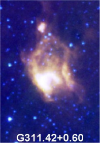
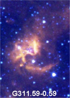
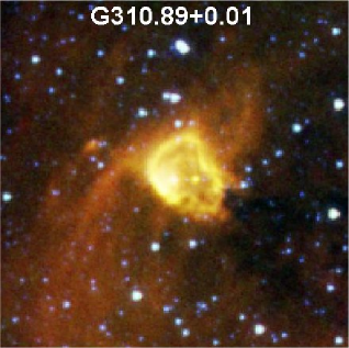
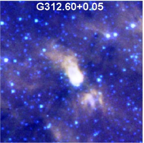
The term “compact Hii region” may be something of a misnomer in the MIR. Each of our radio-compact objects does indeed have a MIR-bright core with apparent scale less than 1^′. Some are well separated from the surrounding ISM (G311.42+0.60, Cs: Fig. 16), but there are often associated multiple centres of emission, intersecting filaments (G311.59$-$0.59, Cf: Fig. 17), and even extended haloes in which 8.0-$\mu$m emission dominates. G310.89+0.01 (Cs: Fig. 18) has a halo in the form of an extensive streamer but its most obvious feature in the MIR is the bright partial shell around its core. G312.60+0.06, (Ch: Fig. 19) is a particularly clear case of a halo around a compact source. It is associated with a small white core (implying MIR thermal continuum) but it is flanked by quite extensive and relatively bright diffuse emission. The haloes could be emitting in PAH bands, H₂ lines or simply be due to continuum from warm ($\sim$350 K) dust grains heated by starlight. The cores of compact Hii regions are generally yellow (PAHs) but some are white, indicative of the role played by thermal emission from hot dust rather than PAHs or any specific fine structure or H₂ emission lines.

Figure 16: Compact Hii region G311.42+0.60 (Cs) with shell and multiple cores. Image is 162 by 288 arcsec.

Figure 17: Compact Hii region G311.59$-$0.59 (Cf), with its filamentary core. Image is 169 by 240 arcsec.

Figure 18: Compact Hii region G310.89+0.01 (Cs), with an extended halo in the form of a streamer, as well as a bright, shell at its core. Image is 240 by 240 arcsec.

Figure 19: Compact Hii region G312.60+0.05 (Ch), with a bright, diffuse halo. Image is 240 by 240 arcsec.

Most shell-type Hii regions consist of bounded ionized zones in the radio and in H$\alpha$ emission. Their MIR counterparts are filamentary PDRs that enclose the ionized gas. Some may include dominant, bright cores (G311.48+0.37, Cs: Fig. 20).

Figure 20: Compact Hii region G311.48+0.37 (Cs) which is dominated by a bright compact region yet incorporates both shells and filaments in the MIR. Image is 720 by 480 arcsec.

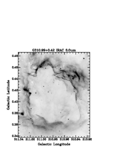
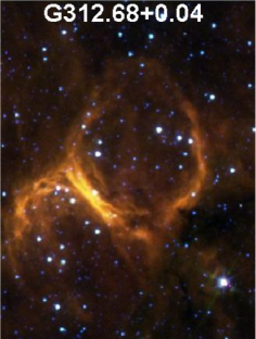
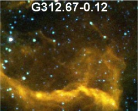
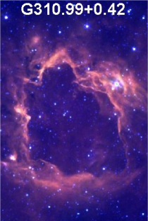
Our sample contains relatively few shell sources. G312.68+0.04 (type Si: Fig. 21) is the north-western of a pair of interacting bubbles. The second object is G312.71+0.02 (Si), south-east of the bright PDR that arises from the interaction of the shells blown by the winds from the two exciting stars. The odd structure, G312.67$-$0.12 (S) (Fig. 22) consists of a bundle of filaments with contiguous diffuse emission, suggestive of a partial shell. As noted by CG, even at the resolution of MSX, the shell comprising the PDR of G310.99+0.42 (S: Fig. 23) is entirely composed of overlapping filaments. These are very well shown at the higher resolution of SST (see also Fig. 1).

Figure 21: Pair of interacting shell regions with bright interaction bar: G312.68+0.04 (Ci) and G312.71+0.02 (Ci). Image is 360 by 480 arcsec.

Figure 22: Partial shell source, G312.67$-$0.12 (S). Image is 288 by 240 arcsec.

Figure 23: Shell Hii region G310.99+0.42 (S). Image is 480 by 720 arcsec.

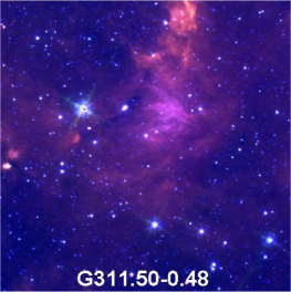
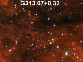
Diffuse regions are the second most numerous morphology in the MIR. Truly diffuse emission (no filaments, shell, or core) is associated with G311.50$-$0.48 (type D:Fig. 24). Most of their MIR emission is diffuse and purple, a colour that might indicate that H₂ lines dominate both the 4.5 and 8.0-$\mu$m bands. Its IRAS LRS spectrum (Fig. 5) is both too noisy and at too poor a spectral resolution to be capable of showing any of these molecular lines. Diffuse regions may contain filaments, such as G313.07+0.32 (Df: Fig. 25). Its MIR emission is red because it is detected only at 8.0-$\mu$m. Fig. 25 is a fine example of an object with so much diffuse PAH emission that it would be almost impossible to determine where the real sky background occurs within this box, in order to set it to a black level.

Figure 24: Diffuse Hii region G311.50$-$0.48 (D). Image is 720 by 720 arcsec.

Figure 25: Diffuse Hii region, G313.07+0.32 (Df), containing filaments. Image is 480 by 360 arcsec.

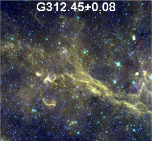
G312.45+0.08 (Fig. 26) is a spectacular network of filaments over 1^∘ in length, containing a pair of braided filaments as if two very large bubbles have come into contact without disruption. The interaction is apparently not vigorous but has led to a warping of the interface between them (CG).

Figure 26: Large filamentary region G312.45+0.08 (F). Image is 70 by 60 arcmin.

Hii regions with compact MIR morphology all have compact (or ultracompact) radio morphology. Filamentary MIR regions are likewise filamentary radio regions. But shells and diffuse regions show no unique relationship between radio and MIR morphologies, most likely because the resolution of the SST is so much higher than that of the MOST, but also because PAHs arise in the neutral zones that surround Hii regions, giving them complementary, rather than identical, structures.

SST’s high resolution implies that one could characterize Hii regions solely using their MIR structure. Kurtz et al. (1999) demonstrated that, in the sample of 15 Hii regions they studied in the radio continuum, extended emission is found in 12 objects. The dynamic range required to detect these haloes can be assessed from their maps given that their contour levels correspond to factors of 2, the lowest levels are given, as are the rms noise values in their Very Large Array (VLA) maps. Typical dynamic ranges are between 60 and 500, calculated as the ratio between the compact peak level and the 3-4 rms contour. The integrated extended emission in a 5 arcmin square centred on the compact components ranges from 1 to 15 times that of the peak intensity, in those objects for which Kurtz et al. (1999) regard a physical association between halo and compact sources to be possible. One third (six regions) of our MIR compact sources show extended emission. The dynamic range in surface brightness from each 8.0-$\mu$m peak to the faintest extended emission clearly detected with IRAC (all quantities are measured above the sky emission) ranges from 8 to 50. The integrated 8.0-$\mu$m brightness of these haloes, compared with a point source matched to the compact peaks’ surface brightness levels, lies between 10 and 140. Thus, the MIR dynamic range probed by the GLIMPSE survey is about 10 times smaller than that at 3.6 cm (the wavelength used by Kurtz and his colleagues). If associated with the compact regions, the MIR haloes would contribute 10 times more flux relative to their compact peaks than at 3.6 cm. If the MIR haloes radiated thermally then the expected 843-MHz continuum from these haloes would be 36 times smaller than that seen by SST (using our median ratio of IRAC/MOST without recalibration). The 3.6 cm radio emission would be 47 times smaller than at 8.0 $\mu$m, with the frequency dependence of the Gaunt factor for a typical Hii region. The average rms noise in the VLA survey fields (Kurtz et al. 1999, their Table 2) is 0.5 mJy beam^-1 so the 3 rms level is about 1.5 mJy beam^-1, equivalent to 38 MJy sr^-1 at 8.0 $\mu$m. The average of the 8.0-$\mu$m sky-subtracted halo brightnesses for the six regions with MIR type “Ch” is 35$\pm$10 MJy sr^-1. Therefore, GLIMPSE at 8.0 $\mu$m provides comparable sensitivity to extended MIR emission around compact Hii regions to that afforded by VLA surveys such as that by Kurtz and colleagues.

Are there MIR haloes akin to the extended weakly ionized radio haloes? Within the ionized gas of an Hii region PAHs suffer photodestruction by UV photons. If any survived, the wind of the central star would rapidly sweep them away into the PDR. Allain, Leach & Sedlmayr (1996a) have shown that small PAHs (those with fewer than 50 carbon atoms) are destroyed by photodissociation on a timescale of a few years in those places in which the characteristic MIR bands are seen, specifically for Hii regions. Cations and partially hydrogenated PAHs may survive for only about a year (Allain, Leach & Sedlmayr 1996b) because they are less stable than the parent molecules. Consequently, small PAHs must be made in abundance in locations in which the MIR bands are emitted, for example in shocks with speeds between 50 and 200 km s^-1 where shattering and fragmentation create PAH molecules, PAH clusters, and small grains (Jones, Tielens & Hollenbach 1996). PAHs with more than 50 carbon atoms may survive the UV radiation field and even small PAHs might last as long as 1000 years in the diffuse ISM. Therefore, PAHs might exist for significant periods in extended haloes that were only weakly ionized and far from the dominant source of destructive UV photons. If all the MIR halo emission were due to PAHs then it would be plausible to associate weak diffuse PAH emission with extended radio haloes in which low fluxes of UV photons leaking from dense ionized cores excite rather than destroy PAHs. MIR spectroscopy of such haloes would be definitive.

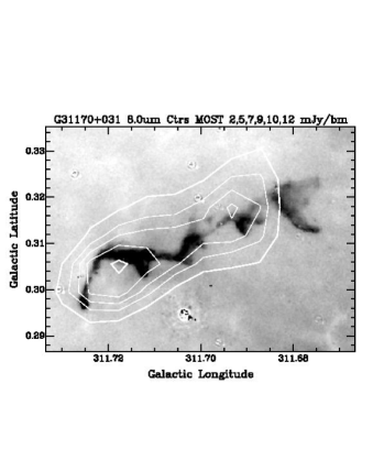
9 G311.70+0.31: a unique structure

Fig. 27 presents the point-source-subtracted image of a most unusual structure in this field, weakly detected by MSX, but clearly present in all four IRAC bands. Its spine consists of a series of segments that strongly suggests that a Rayleigh-Taylor instability might be responsible. If so then the mean wavelength of the segments is 38$\pm$3^′′ (standard error of the mean). However, lacking any estimate of distance and optical forbidden-line spectroscopy, we are unable to use this information on what is surely the fastest growing Rayleigh-Taylor mode to derive a consistent set of physical parameters for the nebula. 843-MHz radio emission was detected by the MOST and is displayed by white contours over the SST 8.0-$\mu$m image. The object’s ratio of MSX 8.3-$\mu$m integrated flux to that from the MOST at 843 MHz is 27$\pm$2, entirely consistent with thermal radio emission and PDRs associated with PAHs. The presence of PAHs is confirmed by the identical morphologies in the IRAC 5.8 and 8.0-$\mu$m bands. The radio emission has two peaks, one within the “bay” of MIR emission to the east, and a second comparable peak west of the centre. A physical association with the east peak is morphologically stronger. If the source represented a structure blown and ionized by a stellar wind then one would expect the hot star to betray its presence by a radio continuum peak and by MIR or far-infrared emission. A search of the region indicates only a single plausible external source that might be a star with a wind, namely IRAS14028$-$6103, a 25-$\mu$m-only object. Nothing definitive can be gleaned from the IRAS photometry or its Low Resolution Spectrum. No counterparts appear in either the 2MASS images or those of the Southern H$\alpha$ Survey (Parker et al. 2005), suggesting high extinction toward the putative MIR and radio source.

Figure 27: Upper: G311.70+0.31 IRAC 8.0-$\mu$m residual image. Circular artefacts are the remnants of point sources that have been subtracted from the original image, in particular a very bright object at (311.704,0.294). Lower: G311.70+0.31 8.0-$\mu$m image overlaid by 843-MHz contours at levels of 2, 5, 7, 10, 12 mJy beam^-1.

Figure 28: SNR G311.52-0.34 4.5-$\mu$m residual image in greyscale, overlaid by 13-cm contours.

Figure 29: SNR G311.52-0.34 false colour image: blue 3.6, green 4.5, red 5.8 $\mu$m. The SNR corresponds to the complete ring around the centre.

10 Galaxies, SNRs, and other nonthermal emitters

GLIMPSE at 8.0 $\mu$m offers a survey three orders of magnitude deeper than MSX at 8.3 $\mu$m. This enables us to probe the MIR/radio ratios for sources other than Hii regions. All five of the suspected background galaxies in the l=312^∘ field, described by CG, were detected by the SST at 8.0 $\mu$m. All appear as point sources and so require no aperture correction. The ratios of IRAC/MOST for G310.86+0.01, G311.54$-$0.02, G312.11$-$0.20, G313.25+0.32, and G313.42+0.09 are 0.080, 0.009, 0.081, 0.019, and 0.034, respectively. The average ratio for these galaxies is 0.04$\pm$0.01, 900 times smaller than the empirical ratio for thermal emission.

If we interpret the extended 8-$\mu$m structure that is associated with radio thermal emission as due to PAHs then it is interesting that even diffuse radio regions in this field have 8-$\mu$m emission. This implies that these patchy zones are not optically thin to ionizing radiation because they apparently have PDRs. Seemingly the only environment in this field that shows a deficit of PAHs (as traced by 8-$\mu$m imagery) is toward SNRs.

Very few SNRs were detected by MSX (Cohen et al. (2005) present an MSX image of Cas-A) and nonthermal emission regions are very faint below 9 $\mu$m, compared with thermal zones. When one might suspect that a nonthermal region was detected it is invariably the case that MSX observed a mixture of thermal and nonthermal filaments but only thermal structures were detected. Two (G310.65$-$0.29, G310.80$-$0.41) of the four SNRs in this field are so confused by diffuse and filamentary thermal emission that no useful measurements or even upper limits can be made of their purely nonthermal portions. The SNR G312.44$-$0.36 is very large (40 arcmin) and its interior includes a considerable amount of diffuse emission, probably thermal, and a considerable number of point and compact sources. These circumstances render it a poor candidate for determining the ratio of nonthermal MIR/radio emission.

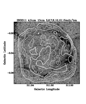
However, the radio-bright young remnant G311.52$-$0.34, discovered by Green (1974), is detected by GLIMPSE. Fig. 28 overlays the 4.5-$\mu$m residual IRAC image by 13-cm continuum contours (ATCA data kindly provided by Josi Gelfand). The spatially integrated, sky-subtracted 8.0-$\mu$m flux density of this SNR can be compared with the integrated radio continuum. The empirical 8.0-$\mu$m to 843-MHz ratio is 0.19, or 0.14 after aperture correction. WCL list one other nonthermal object, G313.45$-$0.13, but this too lies amidst bright thermal filaments. Combining the ratios for the five galaxies with the aperture-corrected ratio for SNR G311.52$-$0.34 yields an average IRAC/MOST ratio of 0.06$\pm$0.02, over 600 times smaller than the thermal ratio. On this basis, the MIR/radio ratio is a sharp discriminant between thermal and nonthermal emission.

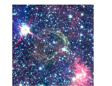
The electronic version of our paper carries a 3-band false colour image (Fig. 29) in which 3.6, 4.5, 5.8-$\mu$m emission are coded blue, green and red, respectively and the remnant can be traced around its complete shell. We have sampled the four brightest areas of MIR emission (roughly one in each quandrant around the elliptical ring) to derive four estimates of IRAC colours for the SNR. The mean values that we calculate yield observed ratios of integrated flux densities at 3.6 and 5.8 $\mu$m of 0.17$\pm$0.06, and at 4.5 and 8.0 $\mu$m of 0.43$\pm$0.06. After applying the SSC aperture corrections these become 0.21$\pm$0.07 and 0.55$\pm$0.08, respectively. Reach et al. (2006) suggest that shocked gas contributes the IRAC emission from this SNR. Our colours, within their uncertainties, overlap the predicted colour-colour box presented by Reach et al. (2006: their Fig. 2) for ionized gas that has suffered a fast shock. The MIR emission is most obvious at 4.5 $\mu$m, and somewhat less bright at 5.8 $\mu$m, due dominantly to Br-$\alpha$ and [Feii] lines, respectively, according to Fig. 1 of Reach et al. (2006).

11 Conclusions

We present evidence that the absolute diffuse calibration of SST at 8.0 $\mu$m is too high by about 36 percent. All measured IRAC surface brightnesses of any diffuse emission region should be scaled down by a multiplicative factor of 0.74$\pm$0.07, based on the absolutely calibrated MSX images. This provides a totally independent confirmation of the separate analyses of IRAC’s diffuse calibration that are based upon the fundamental calibration of the instrument (0.737: Reach et al. 2005) and detailed modeling of the light distributions of elliptical galaxies (0.74$\pm$0.07: Jarrett 2006). Therefore, the recommendation of the SSC that one should scale down 8.0-$\mu$m diffuse BCD flux densities by a multiplicative factor of 0.74 should indeed produce the best absolute estimate of any extended 8.0-$\mu$m emission.

We find that MIR and radio fluxes are linearly related from our regression analysis. These correlations reflect the intimate association between ionized zones and their surrounding PDRs in which polycyclic aromatic hydrocarbon band emission arises. Our median analysis for Hii regions of F_8.3μm/S${}_{843~{}MHz}$ yields 25$\pm$5 (standard error of the median), confirming CG’s original derivation. This ratio of MIR/radio integrated fluxes is independent of morphology of the ionized region but is valid only for radio structures smaller than $\sim$24 arcmin. Aperture synthesis by MOST implies that the telescope is progressively less sensitive to structure on scale sizes $>$15 arcmin, diminishing the estimated fluxes of larger sources. Compact Hii regions below $\sim$3 arcmin in size tend to have somewhat smaller MIR/radio ratios, which might be attributed to absorption by dust grains of UV photons in some of these small, dense regions. The only cometary region in our sample appears to suffer substantial thermal self-absorption of its radio flux.

We find an equivalent correlation for Hii regions between observed 8.0 $\mu$m and 843-MHz fluxes, albeit with more scatter than for MSX. With the SST pipeline and calibration that were applied to the GLIMPSE images released to the community, we find an observed value of F_8.0μm/S${}_{843~{}MHz}$ = 36$\pm$13 best represents this relationship. Removing the 36 percent absolute calibration problem this corresponds to an aperture-corrected ratio for IRAC 8.0/MOST of 27$\pm$10, very similar to the MSX/MOST criterion for radio thermal emission regions. Supernova remnants studied with GLIMPSE images (Reach et al. 2006) show that none has appreciable MIR synchrotron radiation and the dominant post-shock cooling is usually through H₂ lines. This leads to much smaller MIR intensities compared with the radio continuum than for thermal sources, which are intimately associated with PDRs and their bright and broadband PAH emission features. The MIR/radio flux ratio discriminates between thermal and nonthermal regions. For the latter, the ratio is 0.06$\pm$0.02, some 600 times smaller than for Hii regions.

The MIR morphology of Hii regions does not match their radio structure one-to-one. This is most readily seen by examination of Table 1 where the new homogeneous radio and MIR morphologies appear side by side. A diversity of MIR characteristics can be associated with individual radio types. There is clear evidence for extended MIR emission surrounding even compact and cometary Hii regions. Either filaments or diffuse emission may be found around the cores of compact regions, though some appear truly isolated on the sub-arcminute scale. When diffuse MIR structure is found outside the cores of compact Hii regions it has the colour of PAH emission. Consequently, compact Hii regions may indeed have MIR counterparts to the postulated weakly ionized radio haloes. A valid question after examination of these GLIMPSE images is whether there are any compact Hii regions in the MIR without shells, filaments, and haloes. Given the high-resolution of the SST with IRAC one might wish to develop new quantitative criteria for Hii regions, in addition to our MIR morphological characterization.

The SEDs of all the Hii regions in our sample show little variation in the wavelength range seen by the four IRAC bands. Well-defined colours have been determined from this sample, and diagnostic boxes proposed for two IRAC colour-colour planes. There is good separation in these plots between the colours of diffuse thermal emission and those of the plethora of MIR point sources encountered in the Galactic Plane. The colours of known pointlike or ultracompact Hii regions are also sharply distinguished from those of diffuse thermal regions in these plots.

The advantages of combining MIR and radio aspects of particular sources are illustrated by the unique MIR structure of G311.70+0.31 in this field. IRAC’s two longest bands offer a highly sensitive tool for testing for PAH emission by comparing morphologies at different wavelengths that are each dominated by these molecular bands. False colour imagery of G311.70+0.31 shows the excellent match between the MIR configurations of the source at 5.8 and 8.0 $\mu$m, strongly suggestive of the dominance of PAH spectral features in these two images. The flux ratio, MSX/MOST, is exactly what one expects for the combination of thermal radio continuum and 8.3-$\mu$m emission from PAH features. CG emphasized the value of MSX’s filters in which PAH structure detected at 8.3 $\mu$m would be mimicked in the 12.1-$\mu$m image. MSX had a large disparity in responsivity between the 8.3-$\mu$m band and all others, whereas IRAC offers four sensitive detectors so false colour imagery can achieve its true potential.

12 Acknowledgments

MC thanks NASA for supporting this work under LTSA grant NAG5-7936 with UC Berkeley. We are grateful to Tom Jarrett for sharing his extended source calibration results with us, to Masahiro Tanaka for sending us the complete IRTS spectrum of the diffuse ISM, and to Josi Gelfand for sending us the ATCA images of SNR G311.52$-$0.34. We thank the anonymous referee for many valuable and detailed comments and suggestions. This research made use of data products from the Midcourse Space eXperiment. Processing of the data was funded by the Ballistic Missile Defense Organization with additional support from NASA Office of Space Science. This research has also made use of the NASA/IPAC Infrared Science Archive, which is operated by the Jet Propulsion Laboratory, California Institute of Technology, under contract with the National Aeronautics and Space Administration. The MOST is owned and operated by the University of Sydney, with support from the Australian Research Council and Science Foundation within the School of Physics. This research made use of Montage, funded by the National Aeronautics and Space Administration’s Earth Science Technology Office, Computational Technnologies Project, under Cooperative Agreement Number NCC5-626 between NASA and the California Institute of Technology. Support for this work, part of the Spitzer Space Telescope Legacy Science Program, was provided by NASA through contracts 1224653 (Univ. Wisconsin Madison), 1224681 (Univ. Maryland), 1224988 (Space Science Institute), 1259516 (UC Berkeley), with the Jet Propulsion Laboratory, California Institute of Technology under NASA contract 1407. R.I. acknowledges funding as a Spitzer Fellow.

References

- [] Allain, T., Leach, S., Sedlmayr, E. 1996a, A&A, 305, 602
- [] Allain, T., Leach, S., Sedlmayr, E. 1996b, A&A, 305, 616
- [] Assendorp, R., Bontekoe, T.R., de Jonge, A.R.W., Kester, D.J.M., Roelfsema, P.R., Wesselius, P.R. 1995, A&AS, 110, 395
- [] Benjamin, R.A. et al. 2003, PASP, 115, 953
- [] Bock, D.C.-J., Gaensler, B.M. 2005, ApJ, 626, 343
- [] Caswell, J.L. & Haynes, R.F. 1987, A&A, 171, 261
- [] Chiar, J.E., Tielens, A.G.G.M. 2006, ApJ, 637, 774
- [] Churchwell, E.B. et al. 2004, ApJS, 154, 322
- [] Cohen, M. 1993a, AJ, 105, 1860
- [] Cohen, M. 1993b, Final Contractor’s Report and Addendum, USRA Subcontract 5000-02, “Relevance of an Infrared Sky Model to COBE/DIRBE Data Analysis”
- [] Cohen, M. 2000, ”The Diffuse Near- and Mid-Infrared Emission from the Galaxy”, Proc. IAU Symposium 204, ”The Extragalactic Infrared Background and its Cosmological Implications”, eds. Martin Harwit and Michael G. Hauser, p.234
- [] Cohen, M. et al. 2005, ApJ, 627, 446
- [] Cohen, M., Green, A. 2001, MNRAS, 325, 531 [CG]
- [] Cohen, M., Megeath, S. T., Hammersley, P. L., Martin-Luis, F., & Stauffer, J. 2003, AJ, 125, 2645
- [] Cohen, M., Walker, R.G, Barlow, M.J., Deacon, J.R. 1992b, AJ, 104, 1650
- [] Cohen, M., Walker, R. G., Carter, B., Hammersley, P. L., Kidger, M. R., & Noguchi, K. 1999, AJ, 117, 1864
- [] Cohen, M., Walker, R.G, Witteborn, F.C. 1992a, AJ, 104, 2030
- [] Cohen, M., Witteborn, F.C., Carbon, D.F., Davies, J.K., Wooden, D.H., Bregman, J.D. 1996, AJ, 112, 2274
- [] Fazio, G.G. et al. 2004, ApJS, 154, 10
- [] Flagey, N., Boulanger, F., Verstraete, L., Miville Deschenes, M.A., Noriega Crespo, A., Reach, W.T. 2006, astro-ph/0604238 (A&A in press)
- [] Green, A.J. 1974. A&AS, 18, 267
- [] Green, A.J., Cram, L.E., Large, M.I., Ye, T. 1999, ApJS, 122, 207
- [] Hogan, D. 1992, PhD Honour dissertation, Sydney University, Australia
- [] Hora, J. et al. 2004a, IRAC/TM04-010 (June 15, 2004)
- [] Hora, J.L., Latter, W.B., Allen, L.E., Marengo, M., Deutsch, L.K., Pipher, J.L. 2004b, ApJS, 154, 296
- [] Jarrett, T. 2006, private communication
- [] Jones, A.P., Tielens, A.G.G.M., Hollenbach, D.J. 1996, ApJ, 469, 740
- [] Kassis, M., Deutsch, L.K., Campbell, M.F., Hora, J.L., Fazio, G.G., Hoffmann, W.F. 2002, AJ, 124, 1636
- [] Kurtz, S.E., Watson, A.M., Hofner, P., & Otte, B. 1999, ApJ, 514, 232
- [] Murakami, H., Noda, M., Cohen, M., Matsuura, M., 2003, ESA SP-481, ed. L. Metcalfe, pg.423
- [] Olnon, F.M. et al. 1986, A&AS, 65, 607
- [] Onaka, T. et al. 2003, ESA SP-481, ed. L. Metcalfe, pg.119
- [] Parker, Q.A. et al. 2005, MNRAS, 362, 689
- [] Price, S.D., Egan, M.P., Carey, S.J., Mizuno, D., Kuchar, T. 2001, A&A, 121, 2819
- [] Price, S.D., Paxson, C., Engelke, C., & Murdock, T.L. 2004, AJ, 128, p889
- [] Reach, W.T et al. 2005 PASP, 117, 978
- [] Reach, W.T. et al. 2006, AJ, 131, 147
- [] Roche, P.F., Aitken, D.K. 1984, MNRAS, 208, 481
- [] Sakon, I., Onaka, T., Ishihara, D., Ootsubo, T., Yamamura, I., Tanabi, T., Roellig, T.L. 2004, ApJ, 609, 203
- [] Tanabe, T., Yamamura, I., Onaka, T., Chan, K.-W., Roellig, T. L., Cohen, M. 1997, ASP Conf. Ser., 124, 26
- [] Wainscoat, R., Cohen, M., Volk, K.,Walker, H.J., Schwartz, D.E. 1992, ApJS, 83, 111
- [] Walker, H.J., Cohen, M. 1988, AJ, 95, 1801, 1988
- [] Walker, H.J., Cohen, M., Volk, K., Wainscoat, R., Schwartz, D.E. 1989, AJ, 98, 2163, 1989
- [] Werner, M.W. et al. 2004, ApJS, 154, 1
- [] Willner, S. P. et al. 1982, ApJ, 253, 174
- [] Whiteoak, J. B. Z., Cram, L. E., & Large, M. I., 1994, MNRAS, 269, 294 [WCL]
- [] Wildeman, K.J., Beintema, D.A., Wesselius, P.R. 1983, J. Br. Interplanet. Soc., 32, 21