The Faint End of the Luminosity Function in the Core of the Coma Cluster

Abstract

We present optical measurements of the faint end of the luminosity function in the core of the Coma cluster. Dwarf galaxies are detected down to a limiting magnitude of $R\sim 25.75$ in images taken with the Hubble Space Telescope. This represents the faintest determination of the Coma luminosity function to date. With the assumption that errors due to cosmic variance are small, evidence is found for a steep faint end slope with $\alpha\lesssim-2$. Such a value is expected in theories in which reionization and other feedback processes are dependent on density.

1. INTRODUCTION

The galaxy luminosity function (LF) is a fundamental observational probe of galaxy formation and evolution. Defined as the number of galaxies per unit magnitude per unit area on the sky², the LF depends on both the initial density fluctuation spectrum and on baryonic processes such as cooling, star formation and supernova feedback. Any theory attempting to explain how galaxies form and evolve must test its predictions against the observed shape of the LF.

The faint end of the LF is of particular interest. The standard cold dark matter (CDM) model predicts a steep faint end slope to the galaxy LF; the Press-Schechter approximation (1974) combined with a CDM-like power spectrum leads to an increasing number of dark halos as mass scales decrease (White & Rees, 1978). A steep faint end slope has been seen in some environments, mainly those of high density (e.g., Trentham, 1998a; Phillips et al., 1998). In less extreme environments, however, flatter slopes are observed (e.g., Pritchet & van den Bergh, 1999; Trentham et al., 2001). Why are CDM-consistent slopes not seen in all environments?

Studies of the faint end of the LF are hampered by the extreme difficulty of obtaining complete samples of faint, low surface brightness galaxies. It is always possible that the differences in the faint end slope of the LF are simply due to faint galaxies being missed in less dense regions. Other explanations have also been suggested. Tully et al. (2002), for example, use semi-analytic models to show that more low mass halos form earlier in regions that eventually become massive clusters. They then point out that the reionization of the universe could inhibit gas collapse in low mass halos. Combining these ideas, they conclude that dense regions start forming small, faint galaxies before reionization, and so can form many, while less dense regions begin small halo formation later, and so can only form few.

In this work, we examine the faint end of the LF in the core of the Coma Cluster. Coma is a very rich cluster (Abell class 2); Tully et al.’s model would therefore predict Coma to have formed many low mass halos before reionization. We expect to find a steep faint end slope to the Coma LF. We choose to use the method of statistical background subtraction (Zwicky, 1957) to remove background galaxy counts from our sample of cluster galaxy counts: we count the number of galaxies in the cluster direction and then subtract the count of galaxies in a “blank sky” control field.

Many Coma LFs have appeared in the literature (Table 1). This work differs from previous studies in that we use HST images of Coma and of our control field to determine the LF. The increased depth and resolution of these images improves the determination of the faint end slope of the Coma LF.

Table 1Previous studies of Coma’s luminosity function

Study	Passband	Field size	Pixel scale	Lim. mag.	$\alpha$
		(arcmin2)	(arcsec pix-1)	(Vega mags)
Thompson & Gregory 1993	b	14 292	18.56	20	-1.43
Biviano et al. 1995	b	2 496	67.2	20	-1.2 $\pm$ 0.2
Bernstein et al. 1995	R	52.2	0.473	23.5	-1.42 $\pm$ 0.05
Secker et al. 1997	R	$\sim$ 700	0.53	22.5	-1.41 $\pm$ 0.05
Lobo et al. 1997	V	1 500	0.3145	21	-1.8 $\pm$ 0.05
Trentham 1998b	R	674	0.22	23.83	-1.7
Adami et al. 2000	R	52.2	0.473	22.5	-1
Andreon & Cuillandre 2002	B	720	0.206	22.5	-1.25
$\cdots$	V	1 044	0.206	23.75	-1.4
$\cdots$	R	1 044	0.206	23.25	-1.4
Beijersbergen et al. 2002	U	4 680	0.333	21.73	$-1.32^{+0.018}_{-0.028}$
$\cdots$	B	18 720	0.333	21.73	$-1.37^{+0.024}_{-0.016}$
$\cdots$	r	18 720	0.333	21.73	$-1.16^{+0.012}_{-0.019}$
Mobasher et al. 2003	R	3 600	0.21	19.5	$-1.18^{+0.04}_{-0.02}$
Iglesias-Páramo et al. 2003	r’	3 600	0.333	20.5	$-1.47^{+0.08}_{-0.09}$

2. OBSERVATIONS AND DATA REDUCTION

2.1. Coma Data

Our Coma data consist of observations obtained from the HST archive. We selected 16 F606W exposures, totaling 20400 s, and 6 F814W exposures, totaling 7800 s, of a single WFPC2 pointing taken with the center of the PC chip placed on the nucleus of NGC 4874. Due to light contamination from this galaxy, we discarded the PC chip from this project. The combined area of the three WF chips is $\sim 16650$ arcsec² (after trimming), with a plate scale of 0.1^′′ pix^-1. For further details of these observations, see Kavelaars et al. (2000).

The raw data were processed with the standard HST pre-processing pipeline. We then registered the images to within $\sim 0.2$ pix using $\sim 20$ stellar objects on each chip. We scaled the images based on their exposure time and applied a standard cosmic ray rejection algorithm. Finally, we combined the images using the median pixel value, ending with coadded images with effective exposure times of 1300 s.

The coadded Coma images for each chip were dominated with light from a number of bright elliptical galaxies. To remove this light, we used elliptical isophotes to construct photometric models of the six brightest galaxies on the three WF chips. We then subtracted these models from the coadded images. We trimmed the elliptical-subtracted coadded images to remove the regions affected by edge effects, and trimmed the ellipse model images to match. We then ring median-filtered the elliptical-subtracted and trimmed images to create a smoothed map of the background light for each WF chip. We subtracted these background light maps to create final background-subtracted images. We also added the background light map to the trimmed ellipse model image for each chip to create final models of the background for each chip.

2.2. Control Field Data

For control field data, we obtained F606W and F814W images of the Hubble Deep Field North (HDF) (Williams et al., 1996) from the STScI website³. These images had been registered, drizzled onto an image with a sampling of 0.04^′′ pix^-1, background subtracted and normalized to an exposure time of 1 s.

In the method of differential counts, it is imperative to recreate the detection characteristics of the data field as closely as possible in the control field (for a good discussion of this topic, see Bernstein et al. (1995) and Andreon & Cuillandre (2002)). We imposed the Coma pixel scale on the HDF frames by rebinning the images by a factor of 2.5. To match the Coma images’ effective exposure time of 1300 s, we multiplied each HDF image by 1300. We also trimmed the HDF images to match the area of the trimmed Coma images.

To match the noise of the Coma images, we generated a spatially-dependent noise frame for each chip. At each pixel of the noise frame, the expected noise level of the corresponding Coma background model pixel was calculated based on the background level at that pixel, the read noise, and the number of frames that were coadded to create the image. A value for the noise pixel was then drawn at random from a Gaussian distribution centered on zero with standard deviation equal to that expected noise value. The generated value was multiplied by 0.85 a priori to better match the measured noise levels in the background-subtracted Coma images. We added the resulting noise frames directly to the corresponding rebinned, scaled and trimmed HDF chips, as the existing Poisson noise in the HDF images is negligible.

Finally, we subtracted the background of the HDF images in the same manner as the Coma images to keep all processing steps as similar as possible.

3. CREATING THE OBJECT CATALOGS

3.1. Globular Cluster Contamination

One of the advantages of using HST data is its superior resolution over ground-based data. This is important in this work because of the danger of globular cluster blends contaminating the LF. Globular clusters are point sources at the distance of Coma, but two or more globular clusters (or other stellar objects) can appear to be a single extended object when close enough together, and thus be misclassified as a cluster galaxy. This effect was discussed by Andreon & Cuillandre (2002), who noted that a large number of faint, extended objects in their CFHT images of the Coma cluster were resolved into separate point sources in corresponding HST images.

Examination of our preliminary catalogs revealed that while globular clusters were certainly visible as separate point sources, these separate sources would still sometimes be blended into a single object by our detection algorithm. We found this to be a function of the choice of convolution kernel; when the image was convolved with a moderate-sized Gaussian kernel (FWHM $\sim 3$ pix) to enhance detection of extended sources, nearby point sources could be blended into a single extended object (Figure 1). Convolving with a smaller kernel (FWHM $\sim 1.5$ pix) prevented this effect, but using such a small kernel caused some of the more extended faint galaxies to be missed.

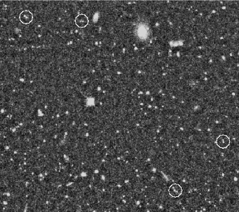
Figure 1.— Blended objects in the Coma catalog. The pairs of point sources circled above are easily resolvable by eye, but were blended into a single extended object by our detection algorithm

To prevent globular cluster blends from contaminating our catalog while still including as many cluster galaxies as possible, we chose to employ a two-pass detection and photometry procedure. We convolved the images once with a small kernel to detect every point source as a separate object. We separated the resulting catalog into “stars” and galaxies on the basis of central concentration, and created a stellar mask for each chip. We applied this mask in a second pass with a larger kernel, such that pixels associated with stellar objects in the first pass could not be detected on the second pass. The results of this second pass then formed our catalog.

The HDF has many fewer point sources than the Coma images, and therefore is much less affected by the danger of point source blends. However, in the interest of processing the data and control images as identically as possible, we applied the same two-pass procedure to the HDF images as well.

3.2. Detection and Photometry

We used the SExtractor package (Bertin & Arnouts, 1996) for detection and photometry. We performed the first detection/photometry pass on the F606W images, convolving with a FWHM = 1.5 pix Gaussian kernel. We set the detection threshold to 1.48 in units of background standard deviation in the unconvolved image; this corresponds to a threshold of $\sim 3.5$ $\sigma$ on the convolved image. We gave the final Coma background model to SExtractor as a variance-type weight map for both the Coma image and the corresponding HDF image. SExtractor uses these weight maps, which describe the noise intensity at each pixel in units of relative weight or relative variance, to slightly adjust the threshold at each pixel to compensate for noise varying across the frame.

To identify the stellar objects in the detection lists, we calculated a “simplified” Petrosian radius $r_{petros}$ for each object. This is defined as the radius at which the function

$$\eta^{\prime}=\frac{F(<r)}{r}$$ (1)

reaches its maximum, where $F(<r)$ is the flux within an aperture with radius $r$. Note that $\eta^{\prime}$ is proportional to signal-to-noise when an image is sky-noise dominated. This measure is loosely based on the Petrosian (1976) radius, which has been used to determine central concentration for various purposes in numerous studies (see, for example, Strauss et al. 2002).

We plotted the $r_{petros}$ for each object versus its MAG  BEST magnitude (Figure 2). We chose a cut of $r_{petros}=1.35$ to separate stellar objects from galaxies. Some stars do fall above this line; however, as the object of this step is to block as many stars as possible while not losing any galaxies, a lower value is preferable. We then used the segmentation image produced by SExtractor to identify the pixels associated with each stellar object. We created a weight map where these pixels were assigned a weight of zero, while the remaining pixels received a weight equal to the inverse of the value of the corresponding Coma background model pixel.

Figure 2.— Simplified Petrosian radius versus instrumental F606W magnitude for objects detected by convolving with a Gaussian kernel of FWHM = 1.5 pix. For the purposes of constructing the globular cluster mask, objects with $r_{petros}\leq 1.35$ are classified as stellar. Some stars do fall above this line; however, a lower value is preferable at this step to block as many stars as possible while not losing any galaxies.

We performed the second detection/photometry pass using this weight map. The image was convolved with a FWHM = 3 pix Gaussian kernel, and we set the detection threshold to 0.86 (again equivalent to $\sim 3.5$ sigma on the convolved image). We set the weight threshold such that no pixels with weights of zero would be included in the detected objects. Photometry was performed on both the F606W and F814W images; object positions and image moments were determined on the (deeper) F606W frames, and then applied to both the F606W and F814W frames to calculate magnitudes. Fixed-aperture magnitudes were also determined in both filters for later use in calculating colors.

3.3. Galaxy Selection

We trimmed the preliminary Coma catalogs to remove objects which fell in the cores of the subtracted Coma elliptical galaxies. The HDF had no large elliptical galaxies to subtract; however, its noise was generated from the Coma background models containing these galaxies, and so we removed HDF objects in the trim regions from the catalogs as well. Finally, to remove any remaining stellar objects from the catalogs, we cut all objects with $r_{petros}\leq 1.55$.

3.4. Limiting Magnitude

We performed add-galaxy experiments to determine the limiting magnitude of our catalogs. For each of 12 0.5 magnitude bins, we generated 100 fake galaxies and added them to one chip of the Coma and HDF images. After running SExtractor on the added-object images, we determined the number of added objects that were recovered. We repeated this process 20 times for both Coma and the HDF and combined the results.

Figure 3 shows the results for both Coma and the HDF. As can be seen, the Coma catalog is over 80% complete to an instrumental F606W magnitude of -4.25. This can then be considered the limiting instrumental magnitude of the catalog.

Figure 3.— Average percentage of added objects recovered in each magnitude bin. Open circles represent the results of objects added to the Coma field; filled squares are the results of objects added to the HDF field. Each point represents the average of 20 runs. Error bars are the standard deviation in the mean.

3.5. Magnitude Transformation

Finally, we transformed our magnitudes to the Vega system Johnson-Cousins B, R and I bands. To transform from instrumental magnitudes to the Vega system, we used the HDF photometric zeropoints on the STScI webpage⁴; to transform from F606W to B and R, and from F814W to I, we used the data of Fukugita et al. (1995). We determined the F606W - F814W color necessary for this transformation from the fixed-aperture magnitudes calculated by SExtractor. To those objects for which SExtractor could not determine fixed-aperture magnitudes, we assigned a color of F606W - F814W = 0.8, chosen as the typical color from a histogram of object colors in the final Coma catalog. Under this transformation, our limiting magnitude (80% completeness) becomes R = 25.75 in the Vega system.

3.6. Color and Morphology

The method of statistical background subtraction can be improved when combined with other forms of background subtraction. A common technique is to pre-select cluster members based on morphology or color before performing the statistical background subtraction. This reduces the number of background galaxies that must be removed statistically, therefore reducing the errors inherent in statistical subtraction.

Unfortunately, the objects found in our Coma fields are too small to derive meaningful morphology information. The objects in the final Coma catalog have a typical effective radius of $\sim 2$ pix. This is simply too few pixels to determine morphological type.

Pre-selecting based on color also proved impossible with these data. Figure 4 shows color-magnitude diagrams of objects in the final Coma and HDF catalogs. As can be seen, the distributions are very similar. There is no obvious way to select Coma cluster members based on their color.

Figure 4.— Color-magnitude diagrams of the final Coma and HDF catalogs. Filled circles represent objects from the Coma catalog; crosses represent objects from the HDF catalog.

3.7. Cosmic Variance

Cosmic variance - the fact that background counts vary from pointing to pointing due to clustering and large scale structure - must be considered when using statistical background subtraction. To understand the effects of cosmic variance on the luminosity function, we evaluated the expression of Peebles (1980) for the variance of the count $N$ of objects in a randomly placed cell. This expression is given by

$$\langle(N-\eta\Omega)^{2}\rangle=\eta\Omega+\eta^{2}\int d\Omega_{1}d\Omega_{2}w(\theta_{12})$$ (2)

where $\eta$ is the mean density of objects on the sky, $\Omega$ is the size of the cell, and $w(\theta_{12})$ is the two-point angular correlation function.

The two-point angular correlation function of galaxies is usually parameterized by $w(\theta_{12})=A_{w}\theta^{-\delta}$, where $A_{w}$ is often a function of magnitude. A search of the literature yielded no applicable studies of the two-point galaxy angular correlation function in the Vega R band. We chose therefore to use the results of Wilson (2003), who did her work in the Vega V band. Wilson’s data can be applied to this work if a constant Vega V-R color is assumed for the objects in the Coma and HDF catalogs. As discussed earlier, the typical Vega F606W-F814W color of objects in the final Coma catalog is 0.8. Using the transformations of Fukugita et al. (1995), this corresponds to a typical Vega V-R color of 0.5. Therefore, Wilson’s coefficients for the bin $m_{1}<V\leq m_{2}$ were applied to the bin $m_{1}-0.5<R\leq m_{2}-0.5$ in this work. The values used can be found in Table 2

For $\eta$, we determined the mean density of background galaxies from the compilation of published field number counts available from the Durham Cosmology Group⁵. Because counts in the Vega V band were not available, the counts in the Vega R band were used. Following the reasoning used above, the counts in the bin $m_{1}-0.5<R\leq m_{2}-0.5$ were used as the counts in the bin $m_{1}<V\leq m_{2}$. From the given data, the average count in each 0.5 mag bin was determined. This value was divided by 3600 to get the average number of galaxies per arcmin² in each bin. As the cosmic variance was to be calculated in 1.0 mag bins, the results from pairs of bins were added together. The resulting values can be found in Table 2.

Finally, for $\Omega$, we simply calculated the total field size of this work by adding together the trimmed areas of the three WF chips. This value can also be found in Table 2

Using these values, we then evaluated Peebles’ integral numerically for each of the four 1.0 magnitude bins. The distance between points was calculated as the linear distance; this approximation is valid for fields as small as the one used here. The resulting values of cosmic variance and standard deviation for each of the bins can be found in Table 2.

Table 2Cosmic Variance

Vega R bin	Vega V bin	$\delta$	log${}_{10}A_{w}(1^{\prime})$	$\eta$	$\Omega$	Cosmic	Standard
				(arcmin-2 mag-1)	(arcmin2)	Variance	Deviation
20.5 - 21.5	21.0 - 22.0	0.8	-1.13 $\pm$ 0.06	1.15	4.62	7.72	2.78
21.5 - 22.5	22.0 - 23.0	0.8	-1.49 $\pm$ 0.05	2.69	4.62	21.3	4.62
22.5 - 23.5	23.0 - 24.0	0.8	-1.72 $\pm$ 0.05	6.37	4.62	48.4	6.96
23.5 - 24.5	24.0 - 25.0	0.8	-2.26 $\pm$ 0.09	14.6	4.62	96.2	9.81

To convert the cosmic variance to an error in the luminosity function, two steps were necessary. First, as the luminosity function was to be expressed in terms of 0.5 mag bins, the error in each 1.0 mag bin due to cosmic variance had to be divided between two bins. We chose to do this based on the relative population of the two bins: If $\sigma_{T}$ is the standard deviation due to cosmic variance for a 1.0 mag bin, and $n_{1}$ and $n_{2}$ are the background counts in two 0.5 mag bins, then the standard deviation due to cosmic variance in the two 0.5 mag bins is given by

$$\sigma_{1} = \sigma_{T}\frac{n_{1}}{n_{1}+n_{2}}$$ (3)

$$\sigma_{2} = \sigma_{T}\frac{n_{2}}{n_{1}+n_{2}}$$ (4)

Second, the error due to cosmic variance only applies to background counts. For the HDF, all the counts in each bin are due to background galaxies. For Coma, however, only a fraction of the counts in each bin are from background galaxies. The exact number for each bin is unknown; statistically, it is assumed to be the same as the HDF count for the corresponding bin. Therefore, we set the error due to cosmic variance for each Coma bin equal to the error due to cosmic variance for the corresponding HDF bin.

We are not able to give an estimate of the cosmic variance all the way down to our limiting magnitude, because Wilson’s study does not go this deep. Therefore, we are forced to assume that the error due to cosmic variance remains small. Further, by using Wilson’s work, we are assuming that the conditions of her study - instrument sensitivity, seeing, detection and photometry algorithm, and so on - are sufficiently similar to the conditions of this study to warrant the comparison.

Obviously, these are very strong assumptions. Ideally, we would evaluate cosmic variance by obtaining additional data taken and reduced under the same conditions of the Coma data. However, this is beyond the scope of this paper, and so we continue under the assumptions stated above.

4. RESULTS

4.1. Comparison to Other Dwarfs

To compare the objects in our Coma catalog to known dwarf galaxies, we collected six published catalogs of dwarf galaxies (Table 3) and obtained the magnitude and half-light radius for each of the galaxies in physical units. When a distance to the group or galaxy was given with the catalog, we adopted that value. For the Virgo cluster, we followed Kavelaars et al. (2000) and used a distance modulus of (m-M) = 30.99.

Table 3Published catalogs of dwarf galaxies

Catalog	Number of galaxies	Reference
Local Group	21	Bender et al. 1992
M101	18	Bremnes et al. 1999
M81	19	Bremnes et al. 1998
Northern Field	17	Barazza et al. 2001
Southern Field	24	Parodi et al. 2002
Virgo Cluster	365	Binggeli & Cameron 1993

We converted the magnitudes and half-light radii of objects in our final Coma catalog into physical units, adopting a distance modulus of (m-M) = 35.05 (Kavelaars et al., 2000). For comparison, we also determined magnitudes and half-light radii for Coma’s globular clusters (i.e., the objects found to be stellar while constructing the globular cluster mask).

Figure 5 shows half-light radius as a function of magnitude for all the objects. Although the Coma galaxies are much fainter than most known dwarf galaxies, they fall in the same general locus. The distribution is understandably more scattered: background galaxies are also present in the Coma catalog, and these show a range of half-light radii at each magnitude. The Coma globular clusters, however, clearly occupy a very different region in the plot. From this plot, we conclude that the objects in the Coma catalog are not globular clusters, and do have the same general morphology as known dwarf galaxies.

Figure 5.— Logarithm of effective radius in kpc versus absolute Vega B magnitude for various dwarfs. Data for dwarfs in Coma are from this work; references for the other catalogs used can be found in Table 3. Also shown for comparison are the Coma globular clusters identified in this work.

4.2. The Luminosity Function

Table 4 shows the data that were used to construct the LF. The number of galaxies in the HDF image is scaled to the unblocked area of the Coma image; the Coma image has many more point sources, and therefore more pixels are blocked by the stellar mask.

Poisson counting errors and errors due to cosmic variance are given separately. The error due to cosmic variance in each 0.5 mag bin could be added in quadrature to the Poisson error. However, the calculation here was performed only to serve as an estimate of the effects of cosmic variance on the slope of the luminosity function. A full treatment would have to account for the correlations in error between magnitude bins introduced by cosmic variance. Due to the simplistic approach and many assumptions used here, we choose to present the two errors separately.

Table 4The luminosity function

$m_{R}$	$N$	$\Delta N_{p}$	$\Delta N_{CV}$	log $\sigma$	$\Delta$log $\sigma$
Coma
20.25	1.00	1.00	$\cdots$	2.89	2.89
20.75	1.00	1.00	1.04	2.89	2.89
21.25	2.00	1.41	1.74	3.19	3.04
21.75	4.00	2.00	2.31	3.49	3.19
22.25	8.00	2.83	2.31	3.79	3.34
22.75	8.00	2.83	2.07	3.79	3.34
23.25	14.00	3.74	4.89	4.04	3.46
23.75	27.00	5.20	3.68	4.32	3.61
24.25	50.00	7.07	6.13	4.59	3.74
24.75	80.00	8.94	$\cdots$	4.79	3.84
25.25	134.00	11.58	$\cdots$	5.02	3.95
25.75	203.00	14.25	$\cdots$	5.20	4.04
Scaled HDF
20.25	1.97	1.39	$\cdots$	3.18	3.03
20.75	2.96	1.71	1.04	3.36	3.12
21.25	4.92	2.20	1.74	3.58	3.23
21.75	6.90	2.61	2.31	3.73	3.31
22.25	6.91	2.61	2.31	3.73	3.31
22.75	10.81	3.26	2.07	3.93	3.40
23.25	25.60	5.02	4.89	4.30	3.59
23.75	20.68	4.51	3.68	4.21	3.55
24.25	34.45	5.82	6.13	4.43	3.66
24.75	78.75	8.81	$\cdots$	4.79	3.84
25.25	70.91	8.36	$\cdots$	4.74	3.81
25.75	107.32	10.28	$\cdots$	4.92	3.90
Coma - Scaled HDF
20.25	-0.97	1.71	$\cdots$	$\cdots$	$\cdots$
20.75	-1.96	1.98	1.48	$\cdots$	$\cdots$
21.25	-2.92	2.62	2.46	$\cdots$	$\cdots$
21.75	-2.90	3.29	3.27	$\cdots$	$\cdots$
22.25	1.09	3.85	3.27	2.93	3.48
22.75	-2.81	4.32	2.92	$\cdots$	$\cdots$
23.25	-11.60	6.26	6.92	$\cdots$	$\cdots$
23.75	6.32	6.88	5.20	3.69	3.73
24.25	15.55	9.16	8.67	4.08	3.85
24.75	1.25	12.55	$\cdots$	2.99	3.99
25.25	63.09	14.28	$\cdots$	4.69	4.05
25.75	95.68	17.57	$\cdots$	4.87	4.14

Note. — The columns are: $m_{R}$ – midpoint of bin in apparent Vega R magnitudes; $N$ – number of galaxies; $\Delta N_{p}$ – Poisson error in the count; $\Delta N_{CV}$ – error due to cosmic variance in the count; log $\sigma$ – logarithmic surface density of objects (number of galaxies per deg²); $\Delta$log $\sigma$ – Poisson error in log $\sigma$.

Figure 6 shows the number counts of the Coma field and the scaled HDF field. As can be seen, cluster counts do not start to dominate over the background until the last two bins. This is due to the small field size surveyed here: cluster galaxies with $20\lesssim R\lesssim 24$ are so rare that $\lesssim$ 1 is expected in a field this size. The galaxies in this magnitude range that are detected in the Coma field are due to background contamination, and so their numbers match those found in the background-only field.

Figure 6.— Number counts from the Coma cluster field and the HDF field (after scaling). Error bars show the Poisson error in the counts.

Figure 7 shows the result of subtracting the HDF counts from the Coma counts – the luminosity function. The shape of the luminosity function is generally parameterized by the Schechter function, which can be written in terms of magnitude as

$$\phi(M)dM\sim 10^{-0.4(\alpha+1)M}e^{-10^{0.4(M^{*}-M)}}$$ (5)

At faint magnitudes, the first term dominates and so the slope of the logarithmic luminosity function is directly related to the parameter $\alpha$. Fitting a straight line to our logarithmic LF using a weighted least-squares fit, we obtain $\alpha=-2.29\pm 0.33$.

Figure 7.— Vega R band luminosity function of the Coma cluster, expressed as logarithmic counts per 0.5 magnitude bin. Error bars show the Poisson error in the counts. The line is a weighted least squares fit to the points.

5. DISCUSSION

5.1. Comparison to Other Work

We have found an extremely steep slope for the faint end of the luminosity function in the Coma cluster. This is especially striking when compared to studies of the faint-end LF in clusters such as Virgo and Fornax. These clusters are close enough that measurements can easily be made at the same absolute magnitudes reached here. For example, in the Virgo cluster, Trentham & Hodgkin (2002) found magnitude-dependent slopes ranging from $-1.49\pm 0.11\leq\alpha\leq-1.02\pm 0.09$ for $-15\leq M_{B}\leq-12$ (roughly equivalent to our absolute magnitude range of $-13\lesssim M_{R}\lesssim-9$). Sabatini et al. (2003) found a slightly steeper slope of $\alpha=-1.6$ for Virgo in the range $-14\leq M_{B}\leq-10$, though this is still significantly flatter than our slope. For Fornax, Hilker et al. (2003) found an extremely flat slope of $\alpha=1.1\pm 0.1$ in the range $-16\lesssim M_{V}\lesssim-9$.

Another interesting comparison is to look at other studies of the LF in the Coma cluster. As noted in the Introduction, many other such studies have appeared in the literature. Table 1 indicates that little consensus has been reached on the “true” slope of the LF. To better compare these studies, we constructed a composite LF.

We obtained background-subtracted number counts for the Coma cluster from the studies listed in Table 1 that were conducted in the R band. We converted the magnitudes to absolute magnitudes using a distance modulus of $(m-M)=34.83$ (Trentham, 1998b). We then scaled the counts and errors to an area of 1 deg², using the field size reported by the authors.

No other normalization was performed. This introduces some scatter to the composite LF; to be perfectly correct, larger surveys – covering more of the low density cluster outskirts and hence having a lower average surface density of galaxies – should be scaled differently than surveys covering only the high density cluster core. However, taking the scale radius (i.e., the radius at which the slope of the profile is the average of the inner and outer slope) of the Coma cluster to be $r_{s}=320$ kpc for H_o = 70 km s^-1 Mpc^-1 (Lokas & Mamon, 2003), the largest survey included here (Mobasher et al., 2003) covers an area roughly 9 times that of the Coma cluster core. Assuming a standard surface density profile ($\sigma(r)=(1+(r/r_{s})^{n})^{-1}$, for $n=1$ or $2$), moving to a radius $\sim 3r_{s}$ would roughly halve the average surface density determined from observing only the cluster core. This corresponds to a scatter of $\pm 0.3$ in our logarithmic composite LF, an acceptable level of error for our purposes.

Figure 8 shows the composite R band luminosity function for the Coma cluster. The bright end shows good agreement among the various surveys. At the faint end, the counts of this work are a clean continuation of the brighter counts from the literature and clearly show a steep faint end slope for the Coma cluster LF.

Figure 8.— The composite Vega R band luminosity function of the Coma cluster, expressed as logarithmic counts per 0.5 magnitude bin and per deg². Bernstein et al.’s “additional counts ” are those not included in their final luminosity function for fear of globular cluster contamination. All counts are scaled to an area of 1 deg²; no other normalization was performed.

Especially interesting are the counts of Mobasher et al. (2003) and Adami et al. (2000). Of the $R$ band studies discussed here, they were the only groups to use spectroscopic redshifts to determine cluster membership. As can be seen in Table 1, their values for $\alpha$ are among the lowest published. This trend of lower $\alpha$ values for spectroscopic studies has sometimes been interpreted as an indication that statistical background subtraction causes artificially steep slopes.

However, looking at the composite LF, the spectroscopic counts of Mobasher et al. agree very well with those obtained by using photometric methods to determine cluster membership. Their counts stop before moving into the truly faint regimes of the LF; spectroscopic studies, by their nature, are limited to bright galaxies and so rarely probe the faint end of the LF. The flatter slopes reported by spectroscopic studies may simply be a result of probing only the brighter, less steeply rising part of the LF.

The counts of Adami et al. do extend into fainter regions of the luminosity function. Their study worked with a small sample of only 88 redshifts. They did not calculate error bars for their luminosity function, but assumed them to be the same as those shown for the (much higher) counts of Bernstein et al. (1995). With these error bars, their counts are consistent at a $1\sigma$ level with those obtained using photometric methods. The general trend of the points may hint at a possible systematic error arising from using photometric methods to construct a luminosity function, but it is dangerous to draw conclusions based on such small numbers and rough error estimates. Unless a larger, better characterized sample of redshifts are obtained which show the same results, we see no compelling evidence that statistical background subtraction leads to an artificially steep LF slope.

Perhaps the most important thing that Figure 8 shows is that, although the various studies did not agree on a value for $\alpha$, the counts themselves agree very well. Caution must always be used when comparing results via parameterized values rather than the underlying data.

5.2. Implications of a Steep Faint-End Slope

We have found a steep faint end slope to the Coma LF. Such steep slopes are not seen in all environments. What could cause this difference between faint end slopes in different environments?

Qualitatively, our results agree with the idea of Tully et al. (2002): Coma, being a rich cluster, formed many dwarf galaxies before reionization “squelched” dwarf galaxy formation. A more quantitative analysis of this idea was performed by Benson et al. (2003). They used detailed semi-analytic models of galaxy formation, including the effects of supernova feedback, photoionization suppression, and dynamical friction and mass loss due to tidal forces, to determine the properties of galaxies in a range of environments. They found that when photoionization suppression was switched on, faint end slopes in poor environments did become flatter than those in rich environments. However, comparing their results to the observational data of Trentham & Hodgkin (2002), they found that photoionization alone cannot flatten the slope enough to match the luminosity functions observed in the Local Group and Ursa Major.

This conclusion is supported by Grebel & Gallagher (2004), who examined the ages of stellar populations in Local Group dwarfs. They found no evidence for a halt or reduction in star formation at $20<z<6.4$, the typical range of epochs for reionization. This indicates that reionization cannot be the dominant influence in the evolution of Local Group dwarfs. Other feedback mechanisms must also be at work.

Obviously, further theoretical efforts are needed to refine the exact processes that shape the luminosity function. Based on the results of this and similar work, these studies must now also explain how these processes can lead to a luminosity function that is different in environments of different densities.

6. CONCLUSION

We have found a steep faint end slope for the galaxy luminosity function in the core of the Coma cluster. Using the method of statistical background subtraction and archival HST images has allowed us to achieve a limiting magnitude of R = 25.75, making this the faintest and highest resolution determination of the Coma luminosity function to date. The fine pixel scale of the WFPC2 camera and our globular cluster mask enabled us to effectively eliminate globular cluster contamination from the final catalog. We find the slope of the luminosity function to be fit by $\alpha=-2.29\pm 0.33$. While this value is not in agreement with other published values of $\alpha$ for the Coma cluster, a composite luminosity function shows our counts to be in good agreement with previous counts. This result could be affected if the errors due to cosmic variance are larger than our estimate. Assuming they are not, the steep slope found in this work is consistent with theories that predict photoionization and other feedback effects will affect environments of low density more severely than environments of high density.

7. ACKNOWLEDGMENTS

This work was supported by the Natural Sciences and Engineering Research Council of Canada (NSERC) through Discovery Grants to CJP and WEH. This work was also supported in part by a Post-Graduate Scholarship to MLM from the NSERC. MLM was a Guest User, Canadian Astronomy Data Centre, which is operated by the Herzberg Institute of Astrophysics, National Research Council of Canada.

References

- Adami et al. (2000) Adami, C., Ulmer, M. P., Durret, F., Nichol, R. C., Mazure, A., Holdne, B. P., Romer, A. K., & Savine, C. 2000, A&A, 353, 930