Photometric follow-up of the transiting planet WASP-1b

Abstract

We report on photometric follow-up of the recently discovered transiting planet WASP-1b. We observed two transits with the Wise Observatory 1m telescope, and used a variant of the EBOP code together with the Sys-Rem detrending approach to fit the light curve. Assuming a stellar mass of $1.15M_{\sun}$, we derived a planetary radius of $R_{p}=1.40\pm 0.06R_{J}$ and mass of $M_{p}=0.87\pm 0.07M_{J}$. An uncertainty of $15\%$ in the stellar mass results in an additional systematic uncertainty of $5\%$ in the planetary radius and of $10\%$ in planetary mass. Our observations yielded a slightly better ephemeris for the center of the transit: $T_{c}$ [HJD] $=(2454013.3127\pm 0.0004)+N_{tr}\cdot(2.51996\pm 0.00002)$. The new planet is an inflated, low-density planet, similar to HAT-P-1b and HD209458b.

1 Introduction

Wide-field small-aperture telescopes are currently used by a few groups (e.g., Bakos et al. 2004, Alonso et al. 2004, McCullough et al. 2005, Pollacco et al. 2006) to search for transiting planetary candidates. However, light curves obtained using wide-field small-aperture telescopes are usually not accurate enough to put useful constraints on the system parameters. Hence, photometric follow-up using larger telescopes is essential.

The WASP consortium (Pollacco et al. 2006) has recently detected two new transiting extrasolar planets, WASP-1b and WASP-2b (Collier Cameron et al. 2006). The discovery paper suggested that WASP-1b is probably an inflated, low-density planet, similar to HAT-P-1b (Bakos et al. 2006) and HD209458b (e.g., Knutson et al. 2006). However, using the photometry of the SuperWASP small-aperture cameras and a single transit observed by a 35cm telescope, Collier Cameron et al. (2006) could not constrain the system parameters of WASP-1 very well. In this work we have set out to better constrain these parameters using the Wise Observatory 1m telescope. We describe our observations in § 2 and the data processing in § 3. In § 4 we briefly discuss our results.

2 Observations

We observed two WASP-1b transits with the 1m telescope at the Wise Observatory, on the nights of 2006 October 4 and 2006 October 9. The observations were carried out in the $I$ filter, with auto-guiding and no defocusing, using a Tektronix $1024\times 1024$ pixel back-illuminated CCD, with a pixel scale of 0.696 arcsec pixel^-1 and an $11.88~{}\times~{}11.88$ arcmin overall field of view (Kaspi et al. 1999).

On 2006 October 4 the exposure time was $60$ seconds at the beginning of the transit, at airmass $\sim 2$, decreasing to $45$ seconds at lower airmass. PSF FWHM was about $2.9$ arcsec that night. On 2006 October 9 exposure time varied between $20$ and $45$ seconds according to varying observing conditions, in particular the bright moon’s altitude. PSF FWHM was about 2.1 arcsec that night. There was a short period of cloudiness on the October 9 night which prevented us from observing the egress of that transit. Nevertheless, we were able to observe the star for a short period after the transit, thus allowing calibration of the light curve zero point.

We did not center the field of view on the target star but instead positioned it at RA = 00h20m21s, DEC = +32^∘02’39” (J2000), in order to include a maximum number of comparison stars, which are essential for the transit light curve reduction.

3 Data processing and model fitting

We used IRAF CCDPROC package for the bias subtraction and flat field correction, using calibration exposures taken nightly. Using the IRAF PHOT task we applied aperture photometry to all field stars in the reduced frames, with a few trial values for the aperture radius and sky annulus size. For the 2006 October 4 frames we obtained the most satisfactory result with an aperture of $7$ arcsec and an annulus inner and outer radii of $35$ and $63$ arcsec, respectively. For the 2006 October 9 frames, an aperture radius of $6$ arcsec and an annulus inner and outer radii of $28$ and $56$ arcsec, respectively, yielded the best result.

Following Winn, Holman and Roussanova (2006), we used nine reference stars and normalized their flux light curves to unit median. We combined these normalized light curves by a simple average and a $3\sigma$ rejection, thus creating a normalized relative flux comparison light curve. We normalized the target star flux light curve by dividing it by the comparison light curve. Finally, we fitted a linear function to the out-of-transit measurements and divided the light curve by this function.

3.1 Photometric parameters

We used the Eclipsing Binary Orbit Program (EBOP) code (Popper & Etzel 1981) together with the Sys-Rem (Tamuz, Mazeh & Zucker 2005; Mazeh, Tamuz & Zucker 2006) code in order to fit the transit light curve to our photometric measurements.

EBOP is widely used for modeling eclipsing binary light curves, and can be easily adapted to model transits (Gimenez 2006). It does not model proximity effects very well, but this is irrelevant for transits. EBOP consists of two modules: a light curve generator and a differential corrections module. Following Tamuz, Mazeh & North (2006) we used only the light curve generator and applied our own optimization program.

Sys-Rem is an algorithm designed to remove systematic effects from photometric light curves without assuming any prior knowledge of the effects. These effects may result from varying observing conditions between observations, such as airmass and weather conditions. Each systematic effect is a sequence of generalized “airmasses” $\{a_{j};j=1,...,M\}$ assigned to each image, where the index $j$ refers to the image number and $M$ is the number of images. Sys-Rem estimates both the effect and a set of coefficients, $\{c_{i};i=1,...,N\}$, which are generalized “colors”, assigned to each star $i$, where $N$ is the number of stars. Essentially, Sys-Rem optimizes the effects and the coefficients such that subtracting the product $c_{i}a_{j}$ from $r_{ij}$, the $j$-th measurement of star $i$, will minimize the RMS of the set $\{r_{ij}-c_{i}a_{j}\}$ (Tamuz et al. 2005).

As a set of photometric measurements can include a few different effects, in our analysis we first estimated $6$ systematic effects for each night separately, using the nine reference stars. Then, we searched for a set of $12$ generalized color coefficients, six for each of the two nights, together with six transit parameters, giving a total of $18$ parameters, that would best fit the target light curve. The six transit parameters included the mid-transit time $T_{c}$, the stellar fractional radius $r_{*}=R_{*}/a$, where $a$ is the orbital semi-major axis, the ratio of planetary radius to stellar radius $k=R_{p}/R_{*}$, the impact parameter $b=\cos i\cdot a/(R_{*}+R_{p})$ and two magnitude zero points for the two nights $I_{1}$ and $I_{2}$.

Transit light curves usually require two additional parameters – the period and a limb-darkening coefficient. We did not optimize for the period and adopted the period published by Collier Cameron et al. (2006). Using the temperature and gravity given by Collier Cameron et al. (2006) we adopted a value of $u=0.37$ (Van Hamme 1993). When $u$ is left as a free parameter, the best-fitting value is $u=0.21\pm 0.08$, which we considered an unphysical result.

Given the $4$ parameters $T_{c}$, $r_{*}$, $k$ and $b$, all the other best-fitting $14$ parameters can be solved for analytically. Thus we can perform a simple grid search over a $4$-dimensional space for the minimum $\chi^{2}$.

After fitting the above model to the data, the residual RMS was found to be $1.8$ mmag in the first night and $2.4$ mmag in the second. We therefore set the photometric errors of each measurement to be equal to the corresponding RMS, and repeated the analysis.

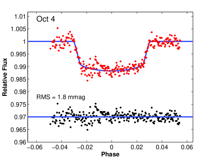
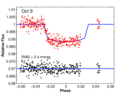
Figure 1: Transit light curves of WASP-1, observed with the Wise Observatory 1m telescope on the nights of 2006 October 4 (left) and 2006 October 9 (right). Relative flux is plotted against orbital phase and the best-fit model is overplotted. Residuals, derived by subtracting the model from the measurements, are plotted at the bottom of each panel and their RMS in each of the light curves is also given.

Table 1 lists all our Sys-Rem–detrended measurements. Table 2 lists the best-fitting values for each of the two transits independently and for both transits simultaneously. We estimated the errors of the best-fitting values using Monte Carlo simulations. We also give the best-fitting values derived without using Sys-Rem, i.e., using only EBOP and no detrending. Accuracy of these parameters is up to seven times better than that of Collier Cameron et al. (2006). We adopted values derived by fitting both nights simultaneously and applying Sys-Rem. Using these parameters we estimate the orbital inclination to be $89.7\pm 1.8$ deg.

Fig. 1 presents our light curves together with the fitted transit model. Fig. 2 presents two $\chi^{2}$ contour maps, from which we can learn about the relations among the best-fitting parameters. The left panel, presenting $\chi^{2}$ as a function of $r_{*}$ and $b$, shows the well known degeneracy of the impact parameter and the stellar radius, while the right panel, presenting $\chi^{2}$ as a function of $r_{*}$ and $k$, shows that the two radii are practically uncorrelated.

Table 1: Table of all 583 photometric measurements. Only the first ten measurements are listed here, the complete table is available in the online version of this article in the Supplementary Materials Section.

HJD - 2454000	Rel. Flux	Err.
13.18941	0.9971	0.0016
13.19324	0.9998	0.0016
13.19432	0.9982	0.0016
13.19537	1.0001	0.0016
13.19642	0.9997	0.0016
13.19749	1.0005	0.0016
13.19854	0.9979	0.0016
13.19960	0.9975	0.0016
13.20065	0.9987	0.0016
13.20171	0.9984	0.0016
⋮	⋮	⋮

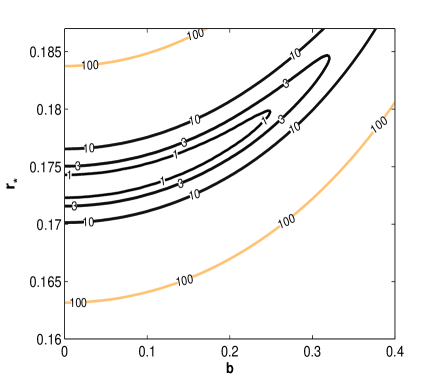
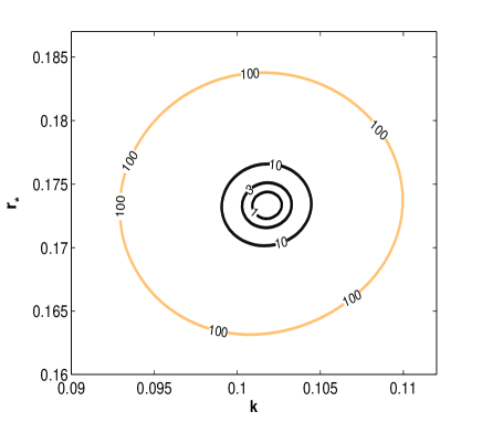
Figure 2: Contour plots of the $\chi^{2}$ function, plotted vs. $r_{*}$ and $b$ (left) and $r_{*}$ and $k$ (right). The contour labels denote the difference between the $\chi^{2}$ of that contour and the minimal $\chi^{2}$.

We used our value of mid-transit time, $T_{c}$, together with the one derived by Collier Cameron et al. (2006) to re-calculate the orbital period, and obtained a value of $2.51996\pm 0.00002$ days. There is no need to re-evaluate all the other parameters, as the errors of the best-fitting parameters are not dominated by the period error.

Our new transit elements allowed us to estimate the transit total duration and duration of ingress and egress. Adopting Eq. 4 of Sackett (1999) for transit duration results in $t_{T}=3.7\pm 0.2$ hours. Assuming transit ingress and egress are symmetric, duration of ingress is calculated by:

$$t_{ingress}=\frac{P}{2\pi}\left[\arcsin(\frac{\sqrt{(R_{*}+R_{p})^{2}-a^{2}\cos(i)^{2}}}{a})-\arcsin(\frac{\sqrt{(R_{*}-R_{p})^{2}-a^{2}\cos(i)^{2}}}{a})\right],$$ (1)

which can be written also as:

$$t_{ingress}=\frac{P}{2\pi}\left[\arcsin(r_{*}(1+k)\sqrt{1-b^{2}})-\arcsin(r_{*}(1-k)\sqrt{1-b^{2}})\right].$$ (2)

In our case $t_{ingress}=20.7\pm 0.9$ minutes.

Table 2: Light curve fitted parameters.

	October 4 transit
	Without Sys-Rem	With Sys-Rem
$r_{*}=R_{*}/a$	$0.180\pm 0.015$	$0.179\pm 0.019$
$k=r_{p}/r_{*}$	$0.101\pm 0.003$	$0.100\pm 0.003$
$b=\cos i\cdot a/(R_{*}+R_{p})$	$0.24\pm 0.19$	$0.23\pm 0.20$
$T_{c}$ [HJD]	$2454013.3131\pm 0.0006$	$2454013.3114\pm 0.0005$
	October 9 transit
	Without Sys-Rem	With Sys-Rem
$r_{*}=R_{*}/a$	$0.187\pm 0.016$	$0.181\pm 0.015$
$k=r_{p}/r_{*}$	$0.107\pm 0.002$	$0.107\pm 0.002$
$b=\cos i\cdot a/(R_{*}+R_{p})$	$0.36\pm 0.20$	$0.24\pm 0.19$
$T_{c}$ [HJD]	$2454013.3124\pm 0.0045$	$2454013.3114\pm 0.0046$
	Both transits
	Without Sys-Rem	With Sys-Rem
$r_{*}=R_{*}/a$	$0.186\pm 0.015$	$0.174\pm 0.007$
$k=r_{p}/r_{*}$	$0.104\pm 0.002$	$0.102\pm 0.001$
$b=\cos i\cdot a/(R_{*}+R_{p})$	$0.34\pm 0.20$	$0.03\pm 0.17$
$T_{c}$ [HJD]	$2454013.3127\pm 0.0005$	$2454013.3127\pm 0.0004$

3.2 Radial-velocity elements

Using the radial-velocity measurements supplied by Collier Cameron et al. (2006) and our improved photometric elements, we were able to re-calculate the radial-velocity elements $K_{1}$, the radial-velocity amplitude, and $\gamma$, the average radial-velocity. The original SuperWASP photometric measurements were obtained two years before the radial-velocities, and therefore did not constrain usefully their orbital phases. Using our ephemeris, we were able to determine the phases of the radial-velocities to a precision of about a minute. Therefore, we have re-calculated the orbital parameters using this constraint. Our derived radial elements are: $K_{1}=118\pm 10$ m s^-1 and $\gamma=-13.506\pm 0.008$ km s^-1.

In order to derive the orbital separation, stellar and planetary radii and the planetary mass we used the stellar mass given by Collier Cameron et al. (2006). As there is a large uncertainty in the stellar mass, we repeated our calculation for the lower and upper limits of the published mass range. The results are given in Table 3. For the most likely value of the stellar mass, the planetary radius and mass are: $R_{p}=1.40\pm 0.06R_{J},M_{p}=0.87\pm 0.07M_{J}$, and the stellar radius is: $R_{*}=1.42\pm 0.06R_{\sun}$. Since stellar and planetary radii scale as $M_{*}^{1/3}$ and the planetary mass scales as $M_{*}^{2/3}$, an uncertainty of 15% on the stellar mass results in an additional systematic uncertainty of 5% on the stellar and planetary radii and of 10% in planetary mass. This systematic uncertainty should be added in quadrature to the errors in Table 3.

Table 3: System parameters derived from the fitted parameters, assuming three different values for the stellar mass. We use the most likely value and the upper and lower limits of Collier Cameron et al. (2006).

$M_{*}$	$a$	$R_{*}$	$R_{p}$	$M_{p}$
$[M_{\sun}]$	$[AU]$	$[R_{\sun}]$	$[R_{J}]$	$[M_{J}]$
1.06	0.037	1.38$\pm$0.06	1.36$\pm$0.06	0.80$\pm$0.07
1.15	0.038	1.42$\pm$0.06	1.40$\pm$0.06	0.87$\pm$0.07
1.39	0.041	1.51$\pm$0.06	1.49$\pm$0.06	1.05$\pm$0.09

4 Discussion

We present here photometry of two transits of the planet WASP-1b, recently published by Collier Cameron et al. (2006). Our new data better constrain the system parameters, mainly the stellar and planetary radii. Combined with previously published results, our new data provide a longer time span, which we use in order to fix the phase of the radial-velocity orbit. Our analysis confirms Collier Cameron et al. (2006) suggestion that the new planet is an inflated, low-density planet. We put all our photometric measurements in the public domain for any further study.

In a simultaneous study, Charbonneau et al. (2006) conducted follow-up observations of WASP-1 and WASP-2, and derived estimates for the stellar and planetary radii with the Mandel & Agol (2002) formulae. Although being slightly larger, their derived radii for the WASP-1 system, of $R_{*}=1.45\pm 0.03R_{\sun}$ and $R_{p}=1.44\pm 0.04R_{J}$, are consistent with ours.

Fig. 3 presents the radii and masses of all currently known transiting planets. The figure shows that WASP-1b radius is similar to HAT-P-1b (Bakos et al. 2006) and HD209458b (e.g., Knutson et al. 2006) radii. This small but growing group of inflated extrasolar planets, whose radii is larger than predicted by common theories of planet formation and evolution (e.g., Laughlin et al. 2005), consists a significant fraction of all currently known transiting planets. A number of possible explanations were suggested to account for this discrepancy between theory and observations by considering, for example, an internal heat source as the cause of these large radii (e.g., Bodenheimer, Laughlin & Lin 2003, Winn & Holman 2005). However, in a recent paper, Burrows et al. (2006) suggest that enhanced planetary atmospheric metallicities, which increase atmospheric opacities, is the underlying mechanism responsible for inflating these extrasolar planets. This explanation does not require any additional heat source and is consistent with the increased probability of high metallicity stars to host planets (Santos et al. 2005, Fischer & Valenti 2005). In addition, Burrows et al. (2006) also pointed out that the commonly used analysis of transiting light curves tend to derive radius larger than the one used in theory, which consider a planet radius till the point where the optical depth in the planet’s atmosphere is $\tau=2/3$.

Combined with all the currently available mass and radius of transiting extrasolar planets, our new values, plotted in Fig. 4, are consistent with the mass-period relation pointed out by Mazeh, Zucker & Pont (2005) and by Gaudi, Seager & Mallen-Ornelas (2005). The only outlier to this relation is HD149026b (Sato et al. 2005) which probably has a dense core (Fortney et al. 2006). We can gain a deeper understanding of this relation and its possible origin by considering the energy diagram of Lecavelier des Etangs (2006, his Fig. 1) presenting the surface potential energy of all extrasolar planets versus the EUV energy flux they receive from their host star. That diagram clearly shows a forbidden region, in which planets with masses too small evaporate because they absorb energy fluxes too large. Maybe the planets can not populate the left-hand bottom of our diagram because of evaporation. However, this scenario does not account for the paucity of transiting planets in the upper right of the diagram. Therefore, we have to find many more transiting planets, in order to verify the mass-period relation and understand its nature.

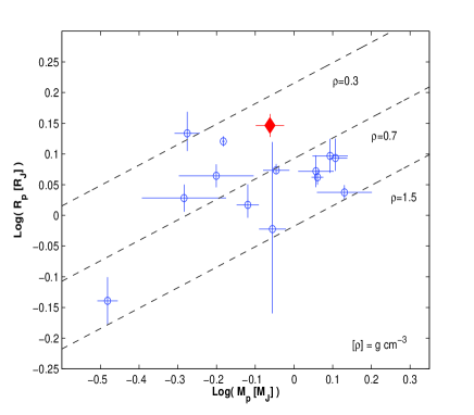
Figure 3: Radius vs. mass of the 14 known transiting extrasolar planets in log-log scale. WASP-1b is marked by a filled diamond. Data for this figure was taken from http://exoplanet.eu/catalog-RV.php.

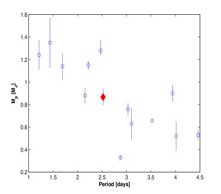
Figure 4: Mass period relation for the 14 known transiting extrasolar planets. WASP-1b is marked by a filled diamond. The planet with the lowest mass, at the bottom of the figure is HD149026b (Sato et al. 2005, Fortney et al. 2006). Data for this figure was taken from http://exoplanet.eu/catalog-RV.php.

References

- (1) Alonso R., et al., 2004, AN, 325, 594
- (2) Bakos G., et al., 2004, PASP, 116, 266
- (3) Bakos G., et al., 2006, ApJ, In press (astro-ph/0609369)
- (4) Bodenheimer P., Laughlin G., Lin D. N. C., 2003, ApJ, 592, 555
- (5) Burrows A., Hubeny I., Budaj J., Hubbard W. B., 2006, ApJ, submitted (astro-ph/0612703)
- (6) Charbonneau D., et al., 2006, ApJ, submitted (astro-ph/0610589)
- (7) Collier Cameron A., et al., 2006, MNRAS, In press (astro-ph/0603688)
- (8) Fischer D. A. & Valenti J., 2005, ApJ, 622, 1102
- (9) Gaudi B. S., Seager S., Mallen-Ornelas G., 2005, ApJ, 623, 472
- (10) Gimenez A., 2006, Ap&SS, 304, 21
- (11) Kaspi S., Ibbetson P. A., Mashal E., Brosch N., 1999, Wise Observatory Technical Report 95/6
- (12) Knutson H., Charbonneau D., Noyes R. W.. Brown T. M., Gilliland R. L., 2006, ApJ, submitted (astro-ph/0603542)
- (13) Laughlin G., et al., 2005, ApJ, 621, 1072
- (14) Lecavelier des Etangs A., 2006, A&A, 461, 1185
- (15) Mazeh T., Zucker S., Pont F., 2005, MNRAS, 356, 955
- (16) Mazeh T., Tamuz O., Zucker S., 2006, astro-ph/0612418
- (17) McCullough P. R., et al., 2005, PASP, 117, 783
- (18) Pollacco D. L., et al., 2006, PASP, 118, 1407
- (19) Popper D. M., Etzel P. B., 1981, AJ, 86, 102
- (20) Sackett P. D., 1999, in Mariotti, J. M., Alloin D., eds, NATO ASIC Proc. 532, Planets Outside the Solar System: Theory and Observations. Kluwer, Boston, p. 189
- (21) Santos N. C., Israelian G., Mayor M., Bento J. P., Almeida P. C., Sousa S. G., Ecuvillon A., 2005, A&A, 437, 1127
- (22) Tamuz O., Mazeh T., Zucker S., 2005, MNRAS, 356, 1466
- (23) Tamuz O., Mazeh T., North, P., 2006, MNRAS, 367, 1521
- (24) Van Hamme W., 1993, AJ, 106, 2096
- (25) Winn J. N. & Holman M. J., 2005, ApJ, 628, L159
- (26) Winn J. N., Holman M. J., Roussanova A., 2006, ApJ, In press (astro-ph/0611404)