Population Boundaries for Galactic White Dwarf Binaries in LISA’s Amplitude-Frequency Domain.

Abstract

Detached, inspiraling and semi-detached, mass-transferring double white dwarf (DWD) binary systems are both expected to be important sources for the proposed space-based gravitational-wave detector, LISA. The mass-radius relationship of individual white dwarf stars in combination with the constraints imposed by Roche geometries permit us to identify population boundaries for DWD systems in LISA’s “absolute” amplitude-frequency diagram. With five key population boundaries in place, we are able to identify four principal population sub-domains, including one sub-domain that identifies where progenitors of Type Ia supernovae will reside. Given one full year of uninterrupted operation, LISA should be able to measure the rate at which the gravitational-wave frequency $f$ and, hence, the orbital period is changing in the highest frequency subpopulation of our Galaxy’s DWD systems. We provide a formula by which the distance to each DWD system in this subpopulation can be determined; in addition, we show how the masses of the individual white dwarf stars in mass-transferring systems may be calculated.

1 Introduction

Double white dwarf (DWD) binaries are considered to be one of the most promising sources of gravitational waves for LISA, the proposed Laser Interferometer Space Antenna (Faller & Bender, 1984; Evans, Iben, & Smarr, 1987; Bender, 1998). If, as has been predicted (Iben & Tutukov, 1984, 1986), close DWD pairs are the end product of the thermonuclear evolution of a sizeable fraction of all binary systems, then DWD binaries must be quite common in our Galaxy and the gravitational waves (GW) emitted from these systems may be a dominant source of background noise for LISA in its lower frequency band, $f\lesssim 3\times 10^{-3}~{}\mathrm{Hz}$ (Hils et al., 1990; Cornish & Larson, 2003). DWD binaries are also believed to be (one of the likely) progenitors of Type Ia supernovae (Iben & Tutukov, 1984; Branch et al., 1995; Tout, 2005) in situations where the accreting white dwarf exceeds the Chandrasekhar mass limit, collapses toward nuclear densities, then explodes. Because its instruments will have sufficient sensitivity to detect GW radiation from close DWD binaries throughout the volume of our Galaxy, LISA will provide us with an unprecedented opportunity to study this important tracer of stellar populations and it will provide us with a much better understanding of the formation and evolution of close binary systems in general. Clearly, a considerable amount of astrophysical insight will be gained from studying the DWD population as a guaranteed source for LISA.

Broadly speaking, our Galaxy’s DWD binary population should be dominated by systems that are in two distinctly different evolutionary phases: An “inspiral” phase, during which both stars are detached from their respective Roche lobes; and a semi-detached, “stable mass-transfer” phase during which the less massive star fills its Roche lobe and is slowly transferring mass to its more massive companion. While DWD binaries may encounter other interesting evolutionary phases – for example, a phase of so-called common envelope evolution, or a phase of rapid, unstable mass transfer – the inspiral and stable mass-transfer phases are expected to dominate the population because they are especially long-lived. It should be noted that we already have a handle on the size of the galactic population of DWD binaries from optical, UV, and x-ray observations. In the immediate solar neighborhood, there are 18 systems (Nelemans, 2005; Anderson, 2005; Roelofs, 2005) known to be undergoing a phase of stable mass transfer (AM CVn being the prototype) and the ESO SN Ia Progenitor SurveY (SPY) has detected nearly 100 detached DWD systems (Napiwotzki et al., 2004b). At present, orbital periods and the component masses for 24 detached DWD systems have been determined (see Table 3 of Nelemans et al. (2005) and references therein), five of which come from the SPY survey.

During both of these relatively long-lived evolutionary phases, a DWD system’s orbital period (and corresponding GW frequency) changes on a time scale that is governed by the rate at which angular momentum is being lost from the system due to gravitational radiation, that is, the so-called “chirp” time scale (see the discussion associated with Eq. 17, below). While the system is detached, the orbital separation slowly decreases so the system should emit a GW signal with a characteristic “chirp” signature, that is, the frequency and amplitude of the GW signal should monotonically increase with time. During a phase of stable mass transfer, however, the orbital separation steadily increases so the GW signal should exhibit an inverse-chirp character where by its frequency and amplitude should steadily decrease with time. The primary objective of our present study is to analyze the imprint that both of these relatively long-lived phases of evolution will have on our Galaxy’s DWD binary population, as viewed by LISA.

LISA’s capabilities as a GW detector are usually discussed in the context of the $\log(h)-\log(f)$ diagram, where the GW frequency $f$ is measured in Hertz, and the GW amplitude $h$ is a dimensionless “strain” (generally quoted per $\sqrt{\mathrm{Hz}}$, reflecting the frequency resolution of the data stream). A useful analogy can be drawn between this amplitude-frequency diagram and the astronomy community’s familiar color-magnitude (CM) diagram. Directly from photometric measurements, astronomers can produce a CM diagram that is based on the apparent brightness (the apparent magnitude $m$) of various sources. However, a determination of the intrinsic brightness of each source must await the determination of the distance $r$ to each source and the corresponding conversion of each measured value of $m$ to an absolute magnitude $M$. LISA’s measurement of $\log(h)$ for a given astrophysical source is analogous to a measurement of $m$; it only tells us how bright the GW source appears to be on the sky. A determination of the intrinsic brightness of each GW source must await a determination of the source distance $r$ and the corresponding conversion of each measured value of (the apparent brightness) $h$ to a quantity that represents the “absolute” brightness of the source. For LISA sources, the relevant quantity (analogous to $M$) is $\log(rh)$. Astronomers realize that the underlying physical properties of stars, their evolution, and their relationship to one another in the context of stellar populations can only be ascertained from a CM diagram if $M$, rather than $m$, is used to quantify stellar magnitudes. By analogy, it should be clear that the underlying physical properties of DWD systems, their evolution, and their relationship to one another in the context of stellar populations can be ascertained only if the observational properties of such systems are displayed in a $\log(rh)-\log(f)$ diagram, rather than in a plot of $\log(h)$ versus $\log(f)$. For this reason, our discussion of DWD systems will be presented in the context of this more fundamental, but rather under-utilized, “absolute” amplitude-frequency domain.

As we investigate the evolution of DWD systems across LISA’s “absolute” amplitude-frequency domain, we will utilize a simplified description of the two long-lived evolutionary phases mentioned above. We will assume (1) all orbits are circular; (2) the orbital frequency is related to the orbital separation via Kepler’s third law; (3) the spin of both stars can be ignored so that each system’s total angular momentum is given by the point-mass expression for orbital angular momentum; (4) the total mass of each system is conserved; and (5) angular momentum is lost from each system only via the radiation of gravitational waves and that the rate of angular momentum loss is correctly described by a quadrupole radiation formula. Simplification #4 means, for example, that after the low-mass white dwarf comes into contact with its Roche lobe, we will assume that each DWD system evolves along a “conservative” mass transfer (CMT) trajectory, and simplification #5 means that we will be ignoring effects that might arise due to direct-impact accretion (Marsh et al., 2004; Gokhale et al., 2006). A more thorough analysis that removes some or all of these simplifications is likely to provide additional valuable insight into the evolution of DWD populations; Stroeer et al. (2005), for example, have expressed concern that the time-rate-of-change of the GW frequency for many of LISA’s most interesting sources will not be correctly interpreted without a proper treatment of tides. In this context, our analysis should be viewed as an important first step in what is likely to be a long-term study of the evolution of the DWD binary population across LISA’s “absolute” amplitude-frequency domain. At the outset, we acknowledge that our understanding of this subject has benefitted significantly from the insight of others whose work has preceded ours; most notably, we recognize the insightful publications by Paczyński (1967), Faulkner (1971), Evans, Iben, & Smarr (1987), Webbink & Iben (1987), Marsh et al. (2004), and Gokhale et al. (2006).

2 Parameterization

In the quadrupole approximation (Peters & Mathews, 1963; Thorne, 1987; Finn & Chernoff, 1993), the time-dependent gravitational-wave strain, $h(t)$, generated by a point mass binary system in circular orbit has two polarization states. The plus and cross polarizations of $h(t)$ generically take the respective forms, $h_{+}=h_{\mathrm{norm}}\cos[\phi(t)]$ and $h_{\times}=h_{\mathrm{norm}}\sin[\phi(t)]$, where the time-dependent phase angle,

$$\phi(t)=\phi_{0}+2\pi\int f(t)dt\,,$$ (1)

where $\phi_{0}$ is the phase at time $t=0$, $f=\Omega_{\mathrm{orb}}/\pi$ is the frequency of the gravitational wave measured in Hz, $\Omega_{\mathrm{orb}}$ is the angular velocity of the binary orbit given in radians per second, and the characteristic amplitude of the wave,

$$h_{\mathrm{norm}}=\frac{G}{rc^{4}}~{}\frac{4\Omega_{\mathrm{orb}}^{2}M_{1}M_{2}a^{2}}{(M_{1}+M_{2})}\,,$$ (2)

where $G$ is the gravitational constant, $c$ is the speed of light, $r$ is the distance to the source, $M_{1}$ and $M_{2}$ are the masses of the two stars, and $a$ is the distance between the stars. If the principal parameters of the binary system do not change with time, then $f$ and $h_{\mathrm{norm}}$ will both be constants and the phase angle $\phi$ will vary only linearly in time, so the source will emit (monochromatic) “continuous-wave” radiation. If, however, any of the binary parameters — $M_{1}$, $M_{2}$, $a$, or $\Omega_{\mathrm{orb}}$ — vary with time, then $h_{\mathrm{norm}}$ and/or $f$ will also vary with time in accordance with the physical process that causes the variation. Here we will only be considering the evolution of DWD systems in which the basic system parameters vary on a timescale that is long compared to $1/f$.

We know from the mass-radius relationship for white dwarfs (see the discussion associated with Eq. 12, below) that the less massive star in a DWD binary will always have the larger radius. Therefore, in a DWD system that is undergoing mass transfer, we can be certain that the less massive star is the component that is filling its Roche lobe and is transferring (donating) mass to its companion (the more massive, accretor). With this in mind, throughout the remainder of our discussion we will identify the two stars by the subscripts $d$ (for donor) and $a$ (for accretor), rather than by the less descript subscripts $1$ and $2$, and will always recognize that the subscript $d$ identifies the less massive star in the DWD system. This notation will be used even during evolutionary phases (such as a GR-driven inspiral phase) when the two stars are detached and therefore no mass-transfer is taking place. Furthermore, we will frequently refer to the total mass of the system, $M_{\mathrm{tot}}\equiv M_{d}+M_{a}$ and the mass ratio,

$$q\equiv\frac{M_{d}}{M_{a}}\,,$$ (3)

which will necessarily be confined to the range $0<q\leq 1$ because $M_{d}\leq M_{a}$. Also, it will be understood that the limiting mass for either white dwarf is the Chandrasekhar mass, $M_{\mathrm{ch}}=1.44M_{\mathrm{\sun}}$.

As mentioned above, throughout this investigation we will assume that Kepler’s third law provides a fundamental relationship between the angular velocity and the separation of DWD binaries, that is,

$$\Omega_{\mathrm{orb}}^{2}=\frac{GM_{\mathrm{tot}}}{a^{3}}\,.$$ (4)

Relation (4) allows us to replace either $\Omega_{\mathrm{orb}}$ or $a$ in favor of the other parameter in Eq. (2). Furthermore, we will find it useful to interchange one or both of these parameters with the binary system’s orbital angular momentum

$$J_{\mathrm{orb}}\equiv\frac{M_{a}M_{d}a^{2}\Omega_{\mathrm{orb}}}{M_{\mathrm{tot}}}=\biggl{(}\frac{G^{2}M_{\mathrm{tot}}^{5}}{\pi f}\biggr{)}^{1/3}Q\,,$$ (5)

where,

$$Q\equiv\frac{q}{(1+q)^{2}}\,,$$ (6)

is the ratio of the system’s reduced mass to its total mass. For our future discussion, it is useful to express the gravitational wave amplitude $h_{\mathrm{norm}}$ and frequency $f$ in terms of $J_{\mathrm{orb}}$ and $Q$. So,

$$h_{\mathrm{norm}} = \frac{4G^{3}}{rc^{4}}\frac{M_{\mathrm{tot}}^{5}Q^{3}}{J_{\mathrm{orb}}^{2}}\,,$$ (7)

$$f = \frac{G^{2}}{\pi}\frac{M_{\mathrm{tot}}^{5}Q^{3}}{J_{\mathrm{orb}}^{3}}.$$ (8)

We note as well that the so-called “chirp mass” $\mathcal{M}$ of a given system (Finn & Chernoff, 1993) is obtained from $M_{\mathrm{tot}}$ and $Q$ via the relation,

$$\mathcal{M}=M_{\mathrm{tot}}Q^{3/5}\,.$$ (9)

3 Evolution of DWD Binaries in the Amplitude-Frequency Domain

3.1 Trajectories and Termination Boundaries

Detached DWD binaries slowly inspiral toward one another as they lose orbital angular momentum due to gravitational radiation. Assuming that $M_{\mathrm{tot}}$ and $q$ remain constant during this phase of evolution, Eqs.(7) and (8) can be combined to give,

$$rh_{\mathrm{norm}} = \biggl{[}\frac{2^{5}\pi^{2}}{c^{2}}\biggl{(}\frac{GM_{\mathrm{ch}}}{c^{2}}\biggr{)}^{5}K^{5}f^{2}\biggr{]}^{1/3}=5.38~{}[K^{5}f^{2}]^{1/3}~{}\mathrm{meters}\,,$$ (10)

where the dimensionless mass parameter,

$$K\equiv 2^{1/5}\biggl{(}\frac{\mathcal{M}}{M_{\mathrm{ch}}}\biggr{)}=2^{1/5}\biggl{(}\frac{M_{\mathrm{tot}}}{M_{\mathrm{ch}}}\biggr{)}Q^{3/5}=\biggl{(}\frac{M_{\mathrm{a}}}{M_{\mathrm{ch}}}\biggr{)}\biggl{(}\frac{2q^{3}}{1+q}\biggr{)}^{1/5}\,,$$ (11)

has been defined such that it acquires a maximum value of unity in the limiting case where $M_{d}=M_{a}=M_{\mathrm{ch}}$; otherwise, $0<K<1$. (We note that in the limiting case of $K=1$, the chirp mass of the system is $\mathcal{M}=0.871M_{\mathrm{ch}}=1.25M_{\odot}$.) From expression (10), we see that the trajectory of an inspiraling, detached DWD binary in the amplitude-frequency diagram can be determined without specifying precisely the rate at which angular momentum is lost from the system. Specifically, because $d\ln(rh_{\mathrm{norm}})/d\ln f=2/3$, trajectories of inspiraling DWD binaries will be straight lines with slope $2/3$ in a plot of $\log(rh_{\mathrm{norm}})$ versus $\log f$. By way of illustration, inspiral trajectories for systems having three different total masses ($2.4~{}M_{\odot}$, $1.4~{}M_{\odot}$, and $0.8~{}M_{\odot}$) but all having the same $q=2/3$ mass ratio are displayed in the top panel of Figure 1.

The detached inspiral phase of the evolution of a DWD binary will terminate when the binary separation $a$ first becomes small enough that the less massive white dwarf fills its Roche lobe. From Eggleton’s mass-radius relationship for zero-temperature white dwarfs, as quoted by Verbunt & Rappaport (1988) and also in Marsh et al. (2004), we know that the radius of the donor $R_{d}$ is,

$$\frac{R_{d}}{R_{\mathrm{\sun}}}=0.0114\biggl{[}\biggl{(}\frac{M_{d}}{M_{\mathrm{ch}}}\biggr{)}^{-2/3}-\biggl{(}\frac{M_{d}}{M_{\mathrm{ch}}}\biggr{)}^{2/3}\biggr{]}^{1/2}\biggl{[}1+3.5\biggl{(}\frac{M_{d}}{M_{\mathrm{p}}}\biggr{)}^{-2/3}+\biggl{(}\frac{M_{d}}{M_{\mathrm{p}}}\biggr{)}^{-1}\biggr{]}^{-2/3}\,,$$ (12)

where $M_{p}\equiv 0.00057~{}M_{\odot}$. Furthermore, from Eggleton (1983) we find that the Roche-lobe radius $R_{L}$ is,

$$R_{\mathrm{L}}\approx a\biggl{[}\frac{0.49\ q^{2/3}}{0.6\ q^{2/3}+\ln(1+q^{1/3})}\biggr{]}.$$ (13)

The orbital separation – and the corresponding GW amplitude $rh_{\mathrm{norm}}$ and frequency $f$ – at which the inspiral phase terminates can therefore be determined uniquely for a given donor mass $M_{d}$ and system mass ratio $q$ by setting $R_{d}=R_{L}$ and combining expressions (12) and (13) accordingly. The termination points of the three inspiral trajectories — marked by plus symbols in the top panel of Figure 1 — have been calculated in this manner. The curve connecting the sequence of plus symbols in Figure 1 traces out the locus of points that define the termination points of the detached inspiral phase of numerous other DWD systems that have mass ratios $q=2/3$ but that have values of $M_{\mathrm{tot}}$ ranging from $2.4~{}M_{\odot}$ to $0.06~{}M_{\odot}$.

As a DWD system fills its Roche lobe and starts transferring mass to its companion, it evolves to lower frequencies and amplitudes. Without knowing the precise rate at which this phase of mass transfer proceeds, we can map out the evolutionary trajectory of various sytems in the $\log(rh_{\mathrm{norm}})-\log f$ diagram if we assume that the system’s total mass is conserved and the donor’s radius is marginally in contact with its Roche lobe. By way of illustration, the bottom panel of Figure 1 shows two stable, conservative mass-transfer (CMT) trajectories: The (blue) dashed trajectory is for a system of mass $M_{\mathrm{tot}}=1.4~{}M_{\odot}$; the (pink) dotted trajectory is for a system of mass $M_{\mathrm{tot}}=0.8~{}M_{\odot}$. We have assumed that both of these systems began the mass-transfer phase of their evolution with an initial mass ratio $q_{0}=2/3$. Hence, the starting point of both trajectories lies on the termination boundary for inspiralling systems having mass ratios of $q=2/3$. For systems with $M_{\mathrm{tot}}>M_{\mathrm{ch}}$, the mass of the accretor will exceed $M_{\mathrm{ch}}$ when $q$ drops below the value,

$$q_{\mathrm{ch}}\equiv\frac{M_{\mathrm{tot}}}{M_{\mathrm{ch}}}-1\,,\qquad\mathrm{for}~{}M_{\mathrm{tot}}>M_{\mathrm{ch}}\,.$$ (14)

With the expectation that something catastrophic (e.g., a Type Ia supernova explosion) will occur when this happens, it is reasonable to assume that CMT trajectories with $M_{\mathrm{tot}}>M_{\mathrm{ch}}$ will terminate at a point in the amplitude-frequency diagram that is marked by $q_{\mathrm{ch}}$. The locus of points that is defined by the termination points of these trajectories defines another interesting astrophysical boundary in LISA’s “absolute” amplitude-frequency diagram. This termination boundary has been drawn as a thick, (green) dashed curve in the bottom panel of Figure 1.

The inspiral trajectory drawn for $K=0.813$ ($M_{\mathrm{tot}}=2.4~{}M_{\odot}$) and the curve marking the termination of various inspiral trajectories in the top panel of Figure 1 define boundaries in the amplitude-frequency domain outside of which no DWD system should exist if it has a mass ratio $q\leq 2/3$. Analogous domain boundaries can be constructed readily for other values of $q$. For each value of $q$, the shapes of the bounding curves are roughly the same as shown in the top panel of Figure 1, but for higher (lower) values of $q$ the right-hand termination boundary shifts to higher (lower) frequencies and the limiting inspiral trajectory (set by the parameter $K$) shifts to higher (lower) strain amplitudes. Given our present understanding of the structure of white dwarfs, it seems extremely unlikely that any DWD binary systems can exist outside of the domain that is defined by the bounding curves for systems with $q=1$ (see, for example, Figure 3).

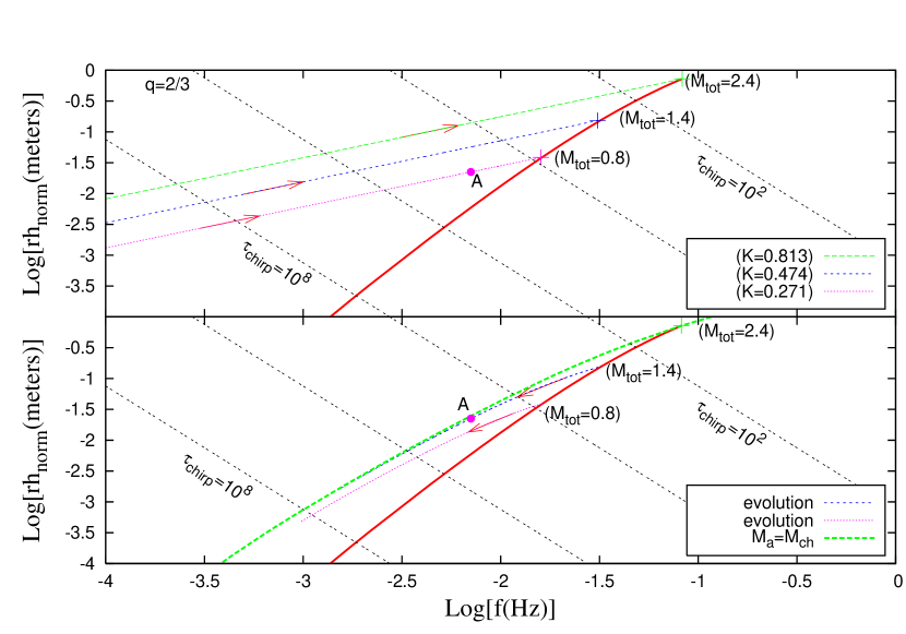
Figure 1: Top panel: Example evolutionary trajectories (lines with arrows pointing to the upper-right) for detached, DWD systems that are undergoing a GR-driven inspiral are displayed in this $\log(rh_{\mathrm{norm}})-\log f$ diagram, where $rh_{\mathrm{norm}}$ is specified in meters and $f$ is specified in Hz. The three trajectories represent systems having dimensionless mass parameters $K=0.813$, $0.474$, and $0.271$ as indicated; assuming a mass ratio $q=2/3$ for all three systems, this corresponds to total system masses of $2.4,1.4$, and $0.8M_{\odot}$, respectively. The termination point of each detached, inspiral trajectory is marked by a plus symbol. The solid red curve passing through the plus symbols forms a termination boundary for inspiraling systems that have a mass ratio $q=2/3$ but a wide range of total masses, $0.06M_{\odot}\leq M_{\mathrm{tot}}\leq 2.4M_{\odot}$; for this mass ratio, $2.4M_{\odot}$ represents the maximum allowed total system mass because $M_{a}=M_{\mathrm{ch}}$. Dotted black lines having a slope of $-2$ depict various “chirp isochrones;” as indicated, the isochones identify systems whose characteristic evolutionary time scales, $\tau_{\mathrm{chirp}}$, range from $10^{2}-10^{8}\textrm{yrs}.$ Bottom panel: In the same $\log(rh_{\mathrm{norm}})-\log f$ parameter space, evolutionary trajectories (curves with arrows pointing to the lower-left) are displayed for DWD systems that are undergoing a stable phase of CMT. The two illustrated trajectories have been drawn for systems that begin their mass-transfer evolutions with a system mass ratio $q_{0}=2/3$ – hence the trajectories begin at the termination points of the respective inspiral trajectories shown above – but they have different total system masses: $M_{\mathrm{tot}}=1.4M_{\odot}$ (blue dotted curve) and $M_{\mathrm{tot}}=0.8M_{\odot}$ (pink dotted curve). The (green) thick dashed curve represents a low-frequency boundary for semi-detached, mass-transferring DWD binaries because, in order for a system to move beyond this boundary, the mass of the accretor $M_{a}$ would have to exceed $M_{\mathrm{ch}}$. The single point marked “A” in both panels $[~{}\log(rh_{\mathrm{norm}}),\log f~{}]=[-1.65,-2.15]$ can represent DWD systems having multiple $(q,M_{\mathrm{tot}})$ pairs.

3.2 Time-Dependence

Up to this point, we have described key features of DWD evolutionary trajectories in LISA’s “absolute” amplitude-frequency diagram without referring to the rate at which the evolution of any given system proceeds. Here we investigate the time scales on which significant changes in various system parameters and, as a consequence, the rate at which measurable changes in the GW signature occur. Using Eqs.(7) and (8), and assuming $M_{\mathrm{tot}}$ as constant, we can write the time-rate-of-change of the amplitude and frequency, for both the inspiral and CMT phase, as follows:

$$\frac{d\ln h_{\mathrm{norm}}}{dt}=-2\frac{\partial\ln J_{\mathrm{orb}}}{\partial t}+3\frac{\partial\ln Q}{\partial t}\,;\qquad\frac{d\ln f}{dt}=-3\frac{\partial\ln J_{\mathrm{orb}}}{\partial t}+3\frac{\partial\ln Q}{\partial t}\,.$$ (15)

During the inspiral phase of DWD binary evolution $\partial\ln Q/\partial t=0$, so the evolution is driven entirely by the loss of angular momentum due to gravitational radiation. According to Peters & Mathews (1963) (see also Misner et al. (1973)), the time-dependent behavior of $J_{\mathrm{orb}}$ is described by the relation,

$$J_{\mathrm{orb}}(t)=J_{0}(1-t/\tau_{\mathrm{chirp}})^{1/8}\,,$$ (16)

where the inspiral evolutionary time scale is,

$$\tau_{\mathrm{chirp}} \equiv \frac{5}{256}\frac{c^{5}a^{4}}{G^{3}M_{\mathrm{tot}}^{3}}\biggl{[}\frac{(1+q)^{2}}{q}\biggr{]}=\frac{5}{64\pi^{2}}\biggl{(}\frac{c}{rhf^{2}}\biggr{)}\,.$$ (17)

Hence,

$$\frac{\partial\ln J_{\mathrm{orb}}}{\partial t}\approx-\frac{1}{8\tau_{\mathrm{chirp}}}.$$ (18)

For the CMT phase, $\partial\ln Q/\partial t\neq 0$. Hence both the terms on the right-hand side of Eq. (15) affect the evolution. From the work of Webbink & Iben (1987) and Marsh et al. (2004), we deduce that during a phase of stable CMT (see Kopparapu (2006) for a detailed derivation),

$$\frac{\partial\ln Q}{\partial t}\approx-\biggl{(}\frac{1-q}{4\Delta\zeta}\biggr{)}\frac{1}{\tau_{\mathrm{chirp}}}\,,$$ (19)

where $\Delta\zeta(M_{\mathrm{tot}},q)\equiv\zeta_{\mathrm{d}}-\zeta_{\mathrm{R_{\mathrm{L}}}}$ is a parameter that is of order unity. The quantities $\zeta_{\mathrm{d}}$ and $\zeta_{\mathrm{R_{\mathrm{L}}}}$ represent the change in the donor’s radius and Roche lobe radius, respectively, as a function of its mass (Marsh et al., 2004). It should be emphasized that the timescale on which DWD systems evolve during both the inspiral and CMT phases is $\sim\tau_{\mathrm{chirp}}$, as indicated by Eqs. (18) and (19). It is for this reason that we have drawn various “chirp isochrones” in both panels of Figure 1; as can be ascertained from Eq.(17), each isochrone depends only on the product of $rh$ and $f^{2}$ and, hence, has a slope of $-2$ in the figure panels.

In practice, for a given source, LISA will be unable to measure changes in the strain amplitude $h$ at the levels predicted by expression (15) because variations in $h$ do not accumulate secularly over time and, in particular, will not contribute to the observed phase of the signal. Since, as indicated in Eq.(1), the phase depends on the time-rate-of-change of the GW frequency we will concentrate on the $d\ln f/dt$ expression in Eq. (15) from here onwards. Combining Eqs. (15), (18) and (19), a concise form of this expression can be written to indicate its behavior during both the inspiral (Nelemans et al., 2001) and CMT (Nelemans et al., 2004) phases as:

$$\frac{df}{dt}=\frac{3f}{8\tau_{\mathrm{chirp}}}\biggl{[}2g-1\biggr{]}$$ (20)

where,

$$g = 0\,\qquad\qquad\qquad(\textrm{inspiral phase});\,$$ (21)

$$g = \frac{(1-q)}{\Delta\zeta}\,\qquad\qquad(\textrm{CMT phase}).$$ (22)

Since $\Delta\zeta$ depends on both $M_{\mathrm{tot}}$ and $q$, there exists a critical $q=q_{\mathrm{crit}}(M_{\mathrm{tot}})$ for which $\Delta\zeta(M_{\mathrm{tot}},q)=0$. For systems with $q>q_{\mathrm{crit}}(M_{\mathrm{tot}})$, a phase of unstable mass transfer ensues and our present analysis becomes invalid in that regime. Hence $q_{\mathrm{crit}}(M_{\mathrm{tot}})$ represents the limiting mass ratio for a system to be in stable CMT phase.

4 Detectability of DWD Systems

4.1 Systems with Non-negligible Frequency Variations

As we have discussed, the physical processes that drive the evolution of DWD binaries operate on a “chirp” timescale, and $\tau_{\mathrm{chirp}}$ is typically much longer than the operational time for LISA (assumed one year here). Hence, the time-variation of a given system’s GW frequency $f(t)$ can be well approximated by a truncated Taylor series expansion in time and, using Eq. (1), the observed phase of the GW signal $\phi_{\mathrm{O}}$ can be written in the form

$$\phi_{\mathrm{O}}(t)=\phi_{0}+2\pi f_{0}t+2\pi\biggl{[}\frac{t^{2}}{2!}\dot{f}+\frac{t^{3}}{3!}\ddot{f}+...\biggr{]}\,,$$ (23)

where $f_{0}$ is the signal frequency at time $t=0$, $\dot{f}=df/dt$, $\ddot{f}=d^{2}f/dt^{2}$, and so on. If we truncate the Taylor series at $\dot{f}$ and this observed signal (O) is compared to a computed template (C) that assumes a continuous-wave signal and therefore has a phase that increases only linearly with time, $\phi_{\mathrm{C}}(t)=(\phi_{0}+2\pi f_{0}t)$, the amount of time for the O-C phase difference to reach $\pi/2$ will be,

$$t_{\mathrm{O-C}}=(2~{}|\dot{f}|)^{-1/2}\,.$$ (24)

Substituting for $\dot{f}$ from Eq. (20), we obtain

$$t_{\mathrm{O-C}}=\biggl{(}\frac{4\tau_{\mathrm{chirp}}}{3|1-2g|f_{0}}\biggr{)}^{1/2}=\biggl{[}\frac{5}{48\pi^{2}|1-2g|}\biggl{(}\frac{c}{rh_{0}f_{0}^{3}}\biggr{)}\biggr{]}^{1/2}\,.$$ (25)

If the function $g$ in Eq.(25) is independent of $h$ and $f$ — as is the case for the inspiral phase of DWD evolutions — then curves of constant $t_{\mathrm{O-C}}$ in the amplitude-frequency diagram will be straight lines having a slope of $-3$. An example of this curve, assuming $t_{\mathrm{O-C}}=1$ year, is shown in Figure 3 joining the two low frequency points. Any inspiral system that lies to the right of this constant $t_{\mathrm{O-C}}$ line will lose phase coherence in less than one year of observation if one assumes that it emits continous-wave radiation. An analogous one-year demarcation boundary can be drawn for DWD binaries that are undergoing a phase of stable, CMT by evaluating Eq. (25) using the function $g(q,M_{\mathrm{tot}})$. Because this function generally is of order unity, the one-year demarcation boundary for mass-transferring systems is generally well-approximated by the line segment that marks the one-year demarcation boundary for inspiral systems. LISA will be able to measure frequency evolution for DWD systems that lie to the right of the $t_{\mathrm{O-C}}=1$ year line and, as will be discussed in the following section, it will then be possible to determine the distances and masses for these systems. The downside is that millions of DWD systems will lie to the left of the one year $t_{\mathrm{O-C}}$ curve in the low frequency region, for which frequency evolution cannot be measured.

4.2 Determination of Distances and Masses

An analysis of a one-year-long LISA data stream that utilizes a proper set of frequency-varying strain templates should be able to determine the rate at which the GW frequency is changing in both inspiral and mass-transfering DWD systems. When used in conjunction with the measurement of $h_{\mathrm{norm}}$ and $f$, an accurate measurement of $\dot{f}$ for any source should permit a determination of the distance to the source $r$ and should give information about the chirp mass $\mathcal{M}$ or the individual component masses of the binary system, as follows.

Equation (10) provides a relation between the three unknown binary system parameters $r,M_{\mathrm{tot}}$ and $q$, and the experimentally measurable parameters $f$ and $h_{\mathrm{norm}}$, namely,

$$\frac{M_{\mathrm{tot}}^{5}}{r^{3}}\biggl{[}\frac{q}{(1+q)^{2}}\biggr{]}^{3} = \frac{\mathcal{M}^{5}}{r^{3}}=\frac{c^{12}}{2^{6}\pi^{2}G^{5}}\biggl{[}\frac{h_{\mathrm{norm}}^{3}}{f^{2}}\biggr{]}\,.$$ (26)

A second relation between the unknown astrophysical parameters and measurable ones is provided by combining the expression for $\dot{f}$ in Eq. (20) with the definition of $\tau_{\mathrm{chirp}}$ given in Eq. (17). Specifically, we obtain,

$$r(1-2g)=\frac{5c}{24\pi^{2}}\biggl{[}\frac{\dot{f}}{h_{\mathrm{norm}}f^{3}}\biggr{]}\,,$$ (27)

With only two equations, of course, it is not possible to uniquely determine all three of the binary’s primary system parameters. However, in the inspiral phase $g=0$, so $\mathcal{M}$ and $r$ can be determined as was shown in Schutz (1986).

During the CMT phase of an evolution, the function $g(M_{\mathrm{tot}},q)$ is nonzero so Eq. (27) does not provide an explicit determination of $r$. However, the requirement that $R_{d}=R_{L}$ provides an important additional physical relationship between the unknown astrophysical parameters and measurable ones. Specifically, by setting $R_{d}$ from Eq. (12) equal to $R_{L}$ from Eq. (13) and using Kepler’s law to write $a$ in terms of $f$, we obtain,

$$\biggl{[}\frac{R_{\mathrm{\sun}}^{3}}{GM_{\mathrm{\odot}}}\biggr{]}^{1/2}f = \biggl{[}\pi^{2}(0.0114)^{3}\frac{M_{\mathrm{ch}}}{M_{\odot}}\biggr{]}^{-1/2}\frac{M_{\mathrm{tot}}}{M_{\mathrm{\odot}}}\biggl{(}\frac{q}{1+q}\biggr{)}H(M_{d},q)\,,$$ (28)

where,

$$H(M_{d},q) \equiv \biggl{(}\frac{1+q}{q}\biggr{)}^{1/2}\biggl{[}\frac{0.49\ q^{2/3}}{0.6\ q^{2/3}+\ln(1+q^{1/3})}\biggr{]}^{3/2}\biggl{[}1-\biggl{(}\frac{M_{d}}{M_{\mathrm{ch}}}\biggr{)}^{4/3}\biggr{]}^{-3/4}$$ (29)

$$\times\biggl{[}1+3.5\biggl{(}\frac{M_{d}}{M_{\mathrm{p}}}\biggr{)}^{-2/3}+\biggl{(}\frac{M_{d}}{M_{\mathrm{p}}}\biggr{)}^{-1}\biggr{]}\,.$$

Hence, taken together, Eqs. (26)-(28) can be used to determine all three primary system parameters – $r$, $M_{\mathrm{tot}}$, and $q$ – from the three measured quantities, $h_{\mathrm{norm}},f$, and $\dot{f}$.

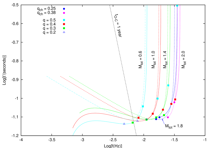
Figure 2: Plot of $\log\Gamma$ versus $\log f$, where $\Gamma\equiv\{[-\dot{f}]^{3}/f^{16}\}^{1/10}$, for stable CMT trajectories having five different system masses ranging from $0.6M_{\odot}$ to $2.0M_{\odot}$, as labeled. Two trajectories are shown for each value of $M_{\mathrm{tot}}$: Dashed curve is the analytic solution provided by Eqs. (30) and (32); solid curve shows the numerical solution obtained from Eqs. (26) through (28). Different values of $q$ are identified by various symbols along each trajectory; note that the trajectories with $M_{\mathrm{tot}}=2M_{\odot}$ and $1.8M_{\odot}$ terminate at values of $q=q_{\mathrm{ch}}=0.38$ and $0.25$, respectively.

We are unable to solve this set of equations analytically due to the complexity of the functions $g(M_{\mathrm{tot}},q)$ and $H(M_{d},q)$. However, the formulae that Paczyński (1967) adopted for $R_{d}(M_{d})$ and $R_{L}(q)$ lead to much simpler expressions for both of these functions, namely, $g=[\frac{3}{2}(1-q)/(2-3q)]$ and $H=1$. In this case Eqs. (26)-(28) can be combined to give $q$ in terms of $f$ and $\dot{f}$:

$$q^{2}(1+q)\biggl{(}1-\frac{3}{2}q\biggr{)}^{3}=\biggl{[}\frac{2^{12}3^{3}\pi^{8}\alpha^{5}}{5^{3}c^{15}}\biggr{]}\frac{f^{16}}{[-\dot{f}]^{3}}\,,$$ (30)

where $\alpha\equiv 0.0141(GM_{\odot}R_{\odot}^{3})^{1/2}$. Once $q$ is known, $r$ can be obtained using Eq.(27) in conjunction with Paczyński’s $g(q)$ relation; then $M_{\mathrm{tot}}$ can be obtained from Eq.(26).

$$r = \frac{5c}{24\pi^{2}}\biggl{[}\frac{-\dot{f}}{h_{\mathrm{norm}}f^{3}}\biggr{]}(2-3q)\,;$$ (31)

$$M_{\mathrm{tot}} = \biggl{[}\frac{5^{3}c^{15}}{2^{15}\cdot 3^{3}\pi^{8}G^{5}}\biggr{]}^{1/5}\biggl{\{}\frac{(1+q)^{6}(2-3q)^{3}}{q^{3}}\cdot\frac{[-\dot{f}]^{3}}{f^{11}}\biggr{\}}^{1/5}\,.$$ (32)

For any $M_{\mathrm{tot}}\leq 2M_{\mathrm{ch}}$, these three equations are valid for mass ratios over the range $0<q<2/3$ because, for Paczyński’s model, $q_{\mathrm{crit}}=2/3$ independent of $M_{\mathrm{tot}}$.

The solid curves in Figure 2 illustrate results obtained numerically from a self-consistent solution of Eqs. (26)-(28); the dashed curves illustrate results obtained analytically from expressions (30) and (32). Across the parameter domain defined by the two observables $\log(f)$ and $\log(\Gamma)$ — where

$$\Gamma \equiv \{[-\dot{f}]^{3}/f^{16}\}^{1/10}\,,$$ (33)

is measured in seconds — each curve traces a constant $M_{\mathrm{tot}}$ “trajectory” with $q$ varying along each curve, as indicated. At high frequencies, each curve begins at a value of $q$ that is slightly below $q_{\mathrm{crit}}$; at low frequencies, the curves have been extended down to $q=0.05$, unless $M_{\mathrm{tot}}>M_{\mathrm{ch}}$, in which case the curve has been terminated at the value $q=q_{\mathrm{ch}}$, as given by Eq. (14). The general behavior of these curves can best be understood by analyzing analytic expression (30). Over the relevant range of mass ratios $0\leq q\leq 2/3$, the analytic function,

$$\Gamma_{\mathrm{anal}} = 0.0521\biggl{[}q^{2}(1+q)\biggl{(}1-\frac{3}{2}q\biggr{)}^{3}\biggr{]}^{-1/10}~{}~{}\mathrm{seconds}\,,$$ (34)

reaches a minimum value ($\Gamma_{\mathrm{min}}=0.077~{}\mathrm{seconds}$) when $q=q_{\mathrm{extreme}}$, where

$$q_{\mathrm{extreme}}\equiv\frac{1}{12}(\sqrt{41}-3)=0.2836\,.$$ (35)

Moving from high frequency to low frequency along each $M_{\mathrm{tot}}$ “trajectory,” the function $\Gamma$ steadily drops until $q=q_{\mathrm{extreme}}$ and $\Gamma=\Gamma_{\mathrm{min}}$. (This behavior holds for the solid curves as well as the dashed curves, although the precise values of $\Gamma_{\mathrm{min}}$ and $q_{\mathrm{extreme}}$ are different for each solid curve.) When $q$ drops below $q_{\mathrm{extreme}}$ [based on the function $q_{\mathrm{ch}}$, this will only happen along curves for which $M_{\mathrm{tot}}<(1+q_{\mathrm{extreme}})M_{\mathrm{ch}}=1.85M_{\odot}$], each curve climbs back above $\Gamma_{\mathrm{min}}$, reflecting the fact that Eq. (30) admits two solutions over the relevant range of mass ratios. This, in turn, implies that for mass-transferring DWD systems that have $\log(f)<-1.74$, a measurement of $\dot{f}$ will generate two possible solutions – rather than a unique solution – for the pair of key physical parameters $(M_{\mathrm{tot}},q)$.

Once LISA has measured $\dot{f}$ as well as $f$ for a given DWD system, Figure 2 provides a graphical means of determining the values of $M_{\mathrm{tot}}$ and $q$ for the system, assuming it is undergoing a phase of stable CMT. We do not expect that LISA will probe the entire parameter space depicted in this figure, however. As discussed above, we expect that LISA will only be able to detect frequency changes in systems for which $t_{\mathrm{O-C}}\lesssim 1~{}\mathrm{yr}$. Using expression (24), this means that LISA will only be able to measure $\dot{f}$ for systems that have,

$$\Gamma\gtrsim 2.57\times 10^{-5}f^{-8/5}~{}\mathrm{seconds}\,.$$ (36)

The dashed black line in Figure 2 with a slope of $-8/5$ that is labeled “$t_{\mathrm{O-C}}=1~{}\mathrm{year}$” shows this boundary; the parameter regime that can be effectively probed by LISA lies above and to the right of this line.

5 Conclusions

5.1 Principal Findings

Once the distance has been determined to individual LISA sources, as was outlined in §4.2, it will be possible to place them in an “absolute” amplitude-frequency diagram, that is, in a $\log(rh_{\mathrm{norm}})-\log(f)$ diagram. The location of individual sources in such a diagram should help us understand a great deal about our Galaxy’s DWD population. Our expectation is that systems in different evolutionary states will fall into several distinct sub-domains of LISA’s “absolute” amplitude-frequency diagram, and the diagram will exhibit natural zones of avoidance as well. Our models of inspiral and CMT systems permit us to predict where the boundaries will lie between these various population sub-domains. As depicted in Figure 3, the principal sub-domains can be identified as follows.

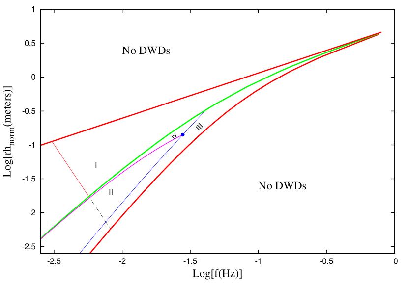
Figure 3: DWD population boundaries are drawn in LISA’s “absolute” amplitude-frequency diagram; five boundary curves (identified as curves A-E in the text) divide the diagram into four principal population sub-domains, numbered $I$-$IV$. Only inspiraling systems will be found in Region I; systems in a phase of stable CMT will only be found in Region II; Region III contains inspiraling systems that will eventually encounter a phase of unstable mass transfer; and systems in Region IV are progenitors of Type Ia supernovae. Zones of Avoidance: As indicated, no DWD systems will be found in the regions that lie outside of the two thick red curves (identified in the text as boundary curves A and B). The straight line of slope $-3$ drawn in the lower left-hand quadrant (identified as curve T in the text) is the $t_{\mathrm{O-C}}=1~{}\mathrm{yr}$ demarcation line; LISA will only be able to measure $\dot{f}$ values for systems that lie above and to the right of this line.

• Zones of Avoidance: No DWD systems will be found in the region above the boundary line that is defined by an inspiral trajectory with $K=1$; according to Eq. (10), this boundary is defined by the expression,

  $$\log(rh_{\mathrm{norm}})=0.731+\frac{2}{3}\log f\,.\qquad{\bf Boundary~{}A}$$ (37)

  Also, no DWD systems will be found in the region below the bounding curve that is defined by the inspiral termination boundary for systems with $q=1$; over the region of parameter space shown in Figure 3 this bounding curve is given approximately by the expression,

  $$\log(rh_{\mathrm{norm}})\approx 0.703 + 0.637~{}\log f-0.017~{}(\log f)^{2}$$ (38)

  $$+ 0.298~{}(\log f)^{3}+0.061~{}(\log f)^{4}\,.\qquad{\bf Boundary~{}B}$$

  Both of these population boundaries have been drawn as solid red curves in Figure 3.

Detached, inspiraling DWD systems will be found throughout the domain whose upper and lower borders are defined, respectively, by boundary curves A and B. This region of parameter space can be subdivided into the following two principal population sub-domains.

• Region I: Only inspiraling DWD systems will be found in the region of parameter space that is bounded above by curve A and below by the locus of points that identifies semi-detached systems for which $M_{a}=M_{\mathrm{ch}}$ (the green solid curve in Figure 3); over the region of parameter space shown in Figure 3, this curve is given approximately by the expression,

  $$\log(rh_{\mathrm{norm}})\approx 0.761 + 1.005~{}\log f+0.700(\log f)^{2}+0.700(\log f)^{3}$$ (39)

  $$+ 0.214(\log f)^{4}+0.023(\log f)^{5}\,.\qquad{\bf Boundary~{}C}$$

• Region II: Mass-transferring DWD systems will only be found in the region of parameter space that is bounded above by curve C and below by curve B.

Region II can be further subdivided into two significant population sub-domains as follows:

• Region III: An inspiraling DWD system that has $q>q_{\mathrm{crit}}(M_{\mathrm{tot}})$ value will encounter an unstable – rather than a stable – phase of mass-transfer when the less massive star initially makes contact with its Roche lobe. The region of parameter space in which these systems will be found at the onset of mass-transfer is bounded below by curve B and above by two intersecting curve segments: At $\log f\gtrsim-1.38$, curve C defines the upper boundary; for $\log f\lesssim-1.38$, the relevant upper boundary has been drawn as a blue solid curve in Figure 3 and is given approximately by the expression,

  $$\log(rh_{\mathrm{norm}})\approx 2.141 + 1.686(\log f)$$ (40)

  $$- 0.141(\log f)^{2}+0.007(\log f)^{3}\,.\qquad{\bf Boundary~{}D}$$

• Region IV: DWD systems that enter a phase of stable CMT with a total system mass $M_{\mathrm{tot}}>M_{\mathrm{ch}}$ will be found in a region of parameter space that is bounded above by curve C and below by two intersecting curve segments: For $-1.55\leq\log f\leq-1.38$, curve D defines the lower boundary; for $\log f\leq-1.55$, the relevant lower boundary has been drawn as a pink solid curve in Figure 3 and is given approximately by the expression,

  $$\log(rh_{\mathrm{norm}})\approx - 1.381-2.108(\log f)$$ (41)

  $$- 1.394(\log f)^{2}-0.167(\log f)^{3}\,.\qquad{\bf Boundary~{}E}$$

  Boundary curve E is defined by the stable CMT trajectory for a system with $M_{\mathrm{tot}}=M_{\mathrm{ch}}$.

An additional demarcation line has been drawn in Figure 3 that is associated with the $t_{\mathrm{O-C}}=1$ yr boundary. This “time boundary” line T is defined by setting $g=0$ and $t_{\mathrm{O-C}}=1$ yr in Eq. (25), that is, it is given by the expression,

$$\log(rh_{\mathrm{norm}})=-8.498-3\log f\,.\qquad{\bf Boundary~{}T}$$ (42)

LISA will be unable to determine distances to DWD systems that lie below and to the left of this demarcation line because their orbital periods and associated GW frequencies are changing so slowly that LISA will be unable to measure with confidence the value of $\dot{f}$ for these systems. Studies of DWD populations will therefore benefit most from the data that LISA collects on systems that lie above and to the right of boundary line T. The segment of this line that bounds Region II has been drawn as a dashed line to emphasize that it is only an approximate one year boundary for mass-transferring systems.

5.2 Discussion

The particular boundaries A-E of the population domains that are depicted in Figure 3 arise as a consequence of the specific mass-radius relationship (Eq. 12) and, hence, the equation of state that we have chosen to use to describe the structure of individual white dwarfs. Because it is generally believed that the mass-radius relationship given in Eq.(12) represents the properties of white dwarfs quite well, we expect that the population sub-domains and zones of avoidance shown in Figure 3 will map well onto LISA’s observationally determined “absolute” amplitude-frequency diagram. Systems that are found on the “wrong” side of a given boundary – for example, any system that lies in one of the zones of avoidance, or CMT systems that are found in Region I – will be of particular interest because they may provide evidence that the equation of state that we adopted is not general enough to properly describe this stellar population Two examples suffice to illustrate this point. First, in the presence of tidal stresses, the donor stars in mass-transferring DWD systems may be hotter than assumed here (Bildsten, 2002; Deloye & Bildsten, 2003), which will affect the frequency at which the donor fills the Roche lobe. Consequently, the inspiral termination boundary B in Figure 3 will change. Second, because individual neutron stars obey an entirely different mass-radius relationship and generally seem to have masses $\gtrsim M_{\mathrm{ch}}$, inspiraling double neutron-star systems will likely be distinguishable from DWD systems because they will lie in the zone of avoidance above boundary curve A, as defined above.

DWD systems that are undergoing a phase of stable, CMT and that are found to reside in Region IV of the “absolute” amplitude-frequency diagram can be identified as progenitors of Type Ia supernovae. Efforts to better understand the origin of supernova explosions in old stellar populations will especially benefit from follow-up studies that identify the optical (or UV or x-ray) counterparts to these Region IV systems. Inspiraling systems that are found to reside in Region III may prove to be equally interesting candidates for follow-up studies. Detached DWD systems in Region III are destined to enter a phase of unstable mass transfer (likely accompanied by super-Eddington accretion, see Gokhale et al. (2006)) that will significantly transform the system’s properties on a dynamical, rather than a chirp, timescale. Such rapid mass-transfer events may lead to merger of the binary components, perhaps followed by an explosion.

As stated above, we are confident that the population sub-domains and zones of avoidance shown in Figure 3 will map well onto LISA’s observationally determined “absolute” amplitude-frequency diagram. We are less confident about the degree to which LISA’s measurements of $\dot{f}$ will match the values that are predicted by our simplified model of the slow, orbit-averaged time-evolution of DWD systems (as displayed, for example, in Figure 2). Mass-transferring binary systems, in particular, are notoriously messy laboratories. For example, significant and unexplained variations in the mass-transfer rate can arise in an individual system over times that are much shorter than the GR-driven evolutionary time scale; this can introduce significant short-term variations in $\dot{f}$. Also, magnetic fields can be effective at carrying away mass and angular momentum from a system, thereby violating our assumption of conservative mass transfer. V407 Vul and RX J0806+1527 (Marsh & Nelemans, 2005) provide perhaps the best examples of the type of confusion that is likely to arise when attempts are made to extract measurements of $\dot{f}$ from a one-year-long LISA data stream. These are optically identified, mass-transferring binaries that are thought to be DWD systems because their orbital periods are less than ten minutes. The best available measurements of period variation in both of these systems indicate that their orbits are slowly shrinking, rather than slowing growing larger as would be predicted by our model of stable CMT. Although, in the mean, the long-term evolutionary behavior of these systems is likely to agree with the predictions of our model, fluctuations about the mean that occur on a timescale that is short compared to $\tau_{\mathrm{chirp}}$ may totally confound our ability to interpret LISA’s measurements of $\dot{f}$. On the bright side, if a significant number of LISA sources exhibit noticeable deviations away from the mean behavior predicted by our simplified model, in the end we are likely to gain a more complete understanding of the evolution of such systems.

References

- Anderson (2005) Anderson, S. F., Haggard, D., Homer, L., Joshi, N. R., Margon, B., Silvestri, N. M., Szkody, P., Wolfe, M. A., Agol, E., Becker, A. C., Henden, A., Hall, P. B., Knapp, G. R., Richmond, M. W., Schneider, D. P., Stinson, G., Barentine, J. C., Brewington, H. J., Brinkman, J., Harvanek, M., Kleinman, S. J., Krzesinski, J., Long, D., Neilsen, E. H. Jr., Nitta, A., & Snedden, S. A. 2005, AJ, 130, 2230
- Bender (1998) Bender, P. L. 1998, BAAS, 193, 48.03
- Bildsten (2002) Bildsten, L. 2002, ApJ, 577, L27
- Branch et al. (1995) Branch, D., Livio, M., Yungelson, L.R., Boffi, F.R., & Baron, E. 1995, PASP, 107, 1019
- Cornish & Larson (2003) Cornish N.J., & Larson S.L. 2003, Phys. Rev. D, 10, 103001
- Cropper et al. (1998) Cropper, M., Harrop-Allin, M, K., Mason, K. O., Mittaz, J. P. D., Potter, S. B., & Ramsay, G. 1998, MNRAS, 293, L57
- Deloye & Bildsten (2003) Deloye, C.J., & Bildsten, L. 2003, ApJ, 598, 1217
- Eggleton (1983) Eggleton, P. P. 1983, ApJ, 268, 368
- Evans, Iben, & Smarr (1987) Evans, C. R., Iben, I., Jr., & Smarr, L. 1987, ApJ, 323, 129
- Faller & Bender (1984) Faller, J. E., & Bender, P. L. 1984, in Precision Measurement and Fundamental Constants II, ed. B. N. Taylor & W. D. Phillips (NBS Spec. Pub. 617)
- Faulkner (1971) Faulkner, J. 1971, ApJ, 170, L99
- Finn & Chernoff (1993) Finn, L.S., & Chernoff, D.E. 1993, Phys. Rev. D, 49, 2658
- Gokhale et al. (2006) Gokhale, V., Peng, X., & Frank, J. 2006, ApJ, submitted
- Hils et al. (1990) Hils, D., Bender, P.L., & Webbink, R.F. 1990, ApJ, 360, 75
- Iben & Tutukov (1984) Iben, I., Jr., & Tutukov, A. V. 1984, ApJS, 54, 335
- Iben & Tutukov (1986) Iben, I., Jr., & Tutukov, A. V. 1986, ApJ, 311, 753
- Kopparapu (2006) Kopparapu, R. K. 2006, Ph.D. Dissertation, Louisiana State University.
- Marsh & Steeghs (2002) Marsh, T. R., & Steeghs, D. 2002, MNRAS, 331, L7
- Marsh et al. (2004) Marsh T. R., Nelemans, G., & Steeghs, D. 2004, MNRAS, 350, 113
- Marsh & Nelemans (2005) Marsh T. R., & Nelemans, G. 2005, MNRAS, 363, 581
- Misner et al. (1973) Misner, C. W., Thorne, K. S., & Wheeler, J. A. 1973, Gravitation (San Francisco: Freeman)
- Napiwotzki et al. (2004b) Napiwotzki, R., Yungelson, L., Nelemans, G., Marsh, T. R., Leibundgut, B., Renzini, R., Homeier, D., Koester, D., Moehler, S., Christlieb, N., Reimers, D., Drechsel, H., Heber, U., Karl, C., & Pauli, E.-M. 2004, ASPC, 318, 402
- Nelemans et al. (2001) Nelemans, G., Yungelson, L. R., & Portegies Zwart, S. F. 2001, A&A, 375, 890
- Nelemans et al. (2004) Nelemans, G., Yungelson, L. R., & Portegies Zwart, S. F. 2004, MNRAS, 349, 181
- Nelemans (2005) Nelemans, G. 2005, ASPC, 330, 27
- Nelemans et al. (2005) Nelemans, G., Napiwotzki, R., Karl, C., Marsh, T. R., Voss, B., Roelofs, G., Izzard, R. G., Montgomery, M., Reerink, T., Christlieb, N., & Reimers, D. 2005, A&A, 440, 1087
- Paczyński (1967) Paczyński, B. 1967, Acta. Astr., 17, 287
- Peters & Mathews (1963) Peters, P.C., & Mathews, J. 1963, Phys. Rev., 131, 435
- Roelofs (2005) Roelofs, G. H. A., Groot, P. J., Marsh, T. R., Steeghs, D., Barros, S. C. C., & Nelemans, G. 2005, MNRAS, 361, 487
- Schutz (1986) Schutz, B. 1986, Nature, 323, 310
- Stroeer et al. (2005) Stroeer, A., Vecchio, A., & Nelemans, G. 2005, ApJ, 633L, 33
- Thorne (1987) Thorne, K. S. 1987, in 300 Years of Gravitation, ed. S. Hawking & W. Israel (Cambridge: Cambridge University Press), 330-458
- Tout (2005) Tout, C. A. 2005, ASPC, 330, 279
- Verbunt & Rappaport (1988) Verbunt, F., & Rappaport, S. 1988, ApJ, 332, 193
- Webbink & Iben (1987) Webbink, R. F., & Iben, I., Jr. 1987, Proceedings of the 2nd Conference on Faint Blue Stars, p. 445
- Wu et al. (2002) Wu, K., Cropper, M., Ramsay, G., & Sekiguchi, K. 2002, MNRAS, 331, 221