Analysis of X-ray flares in GRBs

Abstract

We present a detailed study of the spectral and temporal properties of the X-ray flares emission of several GRBs. We select a sample of GRBs which X-ray light curve exhibits large amplitude variations with several rebrightenings superposed on the underlying three-segment broken powerlaw that is often seen in Swift GRBs. We try to understand the origin of these fluctuations giving some diagnostic in order to discriminate between refreshed shocks and late internal shocks. For some bursts our time-resolved spectral analysis supports the interpretation of a long-lived central engine, with rebrightenings consistent with energy injection in refreshed shocks as slower shells generated in the central engine prompt phase catch up with the afterglow shock at later times

1 Introduction

Most of the Gamma Ray Bursts (GRBs) observed in the pre-Swift era showed a smooth power law decay with time in the X-ray and optical afterglow light-curve [1]. This behavior was found to be consistent with the basic predictions of the fireball model, where the afterglow flux is produced as a relativistic blast wave propagating into an external medium. Under the assumption of a spherical fireball and a uniform medium, Sari, Piran & Narayan (1998) [2] showed that the dependence of the flux on frequency and time can be represented by several power law segments, $F_{\nu}\propto\nu^{-\beta}t^{\alpha}$, each of which applies to a different regime. Before Swift only a few GRBs showing deviations from the smooth power law light curve were known, see e.g. the case of GRB 021004 [3],[4].

This simple picture is now changing since the advent of Swift. Erratic X-ray flares have been detected by Swift in almost half of its GRBs ([5], [6], [7], [8], [9]). While some bursts show one distinct flare after the GRB prompt emission, (e.g. GRB 050406 [10]), other events like GRB 050502B and GRB 050713A, show several flares [6], [9], [7]. One of the main goals of current GRB science is to understand the origin of this newly observed light curve behavior. Since flares are likely to trace the activity of the central engine, they can help us gain insights on the physical processes governing the early post-GRB phases. Note that flares have been observed in the light curves of both long and short GRBs. As a first step toward the understanding of different flares characteristics it is fundamental to carry out a systematic investigation of the morphological and timing properties of the flares observed by Swift/XRT (Chincarini et al. 2006[28]).

In some cases we can already rule out some models that have been proposed to explain the flare phenomenon. The presence of several flares in one GRB strongly disfavors scenarios that can only account for one flare, e.g. the self synchrotron Compton emission from reverse shock [11]. Density bumps [12] cannot be responsible of large amplitude rebrightenings (e.g. GRB 050502B [7]) . In this paper we carry out a detailed spectral and timing analysis of flares in several GRBs with the goal of constraining the physical mechanism responsible for its production. In particular we concentrate on two models proposed for the flares, the late internal shock (IS) model and the refreshed shocks (RS) model.

In the internal shock scenario the flares are due to the reactivation of the GRB central engine and they are produced from an “internal” dissipation radius within the external blast wave front [13]. In this case a mechanism to reactivate the engine is required. For the long bursts, King et al. (2005) [14] proposed a model in which the flares could be produced from the fragmentation of the collapsing stellar core in a modified hypernova scenario. For the case of short GRBs, MacFadyen et al. (2005) [15] suggested that the flares could be the result of the interaction between the GRB outflow and a non-stellar companion. More recently, Perna et al. (2006) [16] have analyzed the observational properties of flares in both long and short bursts, and suggested a common scenario in which flares are powered by the late-time accretion of fragments of material produced in the gravitationally unstable outer parts of an hyper-accreting accretion disk. Other mechanisms that could produce flares involve a magnetic origin [17], [18].

In the refreshed shock scenario [19] the flares are due to late time energy injections into the main afterglow shock by slow moving shells ejected from the central engine during the prompt phase. In this case we do not need a reactivation of the engine. This model can interpret several flares features [20], [21] seen in some GRBs.

Both models have observational consequences that can be tested. In this paper we propose and exploit some diagnostics between the two models.

2 The sample and the data analysis

We consider all the GRBs detected by Swift between the Swift launch and 2006 January 31. We select all those that showed prominent flares in their X-ray lightcurves. In table 1 we list all the GRBs that were selected for the analysis. A more extensive analysis that will be presented includes a larger sample of Swift GRBs [22]. The X-ray data were reduced using the Swift Software (v. 2.0) and in particular the XRT software developed at the ASDC and HEASARC [23] .

Important information on the mechanism producing the flares can be obtained from the comparison between the observed variability timescale $\Delta T$ and the time $T$, at which the flare is observed. In the refreshed shock scenario the early afterglow has a variability timescale of the order of the time since the explosion, $\Delta T\sim T$ [19], while in the late internal shock model $\Delta T<<T$. We calculated for all the flares of the sample the ratio between the duration of the flare, $\Delta T$, and the time at which the flare peaks $T_{\rm peak}$ and report these values in Table 1. We also report the time at which the rising behavior of the light curve begins $T_{\rm rise}$. In our analysis $\Delta T$ is defined as the difference between the times at which the light curve shows the end of the falling and the beginning of the rising behaviors. All times refer to the BAT trigger. As we can see from this table, within the uncertainties, all flares have $\Delta T/T_{\rm peak}\sim O(1)$, in agreement with the refreshed shock scenario. However some of these flares have other characteristics that can be better explained in the internal shock scenario.

The strategy for our temporal fitting procedure is the following. We consider the data in the range between $T_{\rm rise}$ and $T_{\rm peak}$ to compute the slope,$\alpha_{r}$, of the rising part of the light curve. The start time is set to $T_{\rm rise}$. For the decay, we use the data in the range between $T_{\rm peak}$ and the end of the decaying behavior to estimate the power law decay index $\alpha_{d}$. The start time has been set to $T_{\rm peak}$. We note that the power-law rise and decay indices depend strongly on the initial counting time, $T_{0}$. In the internal shock scenario, the re-starting of the central engine re-sets the starting time. This is why some authors [24] use $T_{0}\sim T_{\rm rise}$ to estimate $\alpha_{d}$ and thus find much steeper temporal slopes (we call these slopes $\alpha_{\rm d,IS}$). We think that the right choice for the start time is $T_{\rm peak}$. This is because a start time earlier than the beginning of the decaying behavior causes an unphysical steepening of the slope, due only to mathematical effects. In any case, since the $T_{0}$ issue is an open problem, we also discuss what happens to the decay slope if the start time is set to $T_{\rm rise}$. We therefore report both $\alpha_{d}$ and $\alpha_{\rm d,IS}$ for the bursts were the internal shocks better interpret the flare phenomenology.

2.1 Time-resolved spectroscopy

The analysis of the window timing (WT) light curves of the flares reveal complex spectral variations. To investigate the nature of these variations we performed a time resolved spectral analysis. We first fitted the spectra in the rise and decay parts with a simple power law combined with photoelectric absorption. We indicate with $\Gamma=\beta+1$ the photon index. The results of our fits are shown in Table 2. Large spectral variations are evident, in particular between the spectra corresponding to the rise and fall of several flares.

Motivated by the synchrotron emission model [2], we then fitted the spectra using a broken power law model. We kept the low energy (before the cooling frequency) spectral power law index fixed at $\beta_{1}=\Gamma_{1}-1=0.5$, as expected from standard synchrotron models and left the high energy power law index $\beta_{2}=\Gamma_{2}-1$ as a free parameter. The results are shown in Table 2. In some cases we were not able to fit the spectrum with a broken power law, as evident in Table 3 (we write “na” in this case).

Table 1: values of z, $\Delta T$, $T$ for each flare

GRB	z	$T_{\rm rise}$	$T_{\rm peak}$	$\Delta T$	$\Delta T/T_{\rm peak}$
050406		132	212	160	0.75
050502B		468	848	700	0.83
050713A		97	107	50	0.47
050730(1)	3.97	202	232	100	0.43
050730(2)	3.97	302	432	300	0.69
050730(3)	3.97	602	672	340	0.51
050822		211	231	70	0.30
050904	6.29	368	458	200	0.44
050908		268	388	500	1.29
060111A		204	274	260	0.95
060124(1)		311	571	330	0.58
060124(2)		641	701	230	0.33

3 Refreshed or late internal shocks?

In this section we try to distinguish between the two (IS and RS) models using the temporal and spectral properties derived for each flare in the previous section. As we have emphasized, the parameter that helps in this analysis is the flare duration, $\Delta T$.

3.1 Late-time “energy injection”

If $\Delta T\sim T$ rebrightenings and bumps in the afterglow light curve may be due to “energy injections” at later times that could be produced by slower shells that catch up with the afterglow shock at later times. In this case we have some predictions on how the temporal and the spectral energy slope should be related. We consider the standard afterglow model in the adiabatic evolution [2]. The analysis can be easily extended to the radiative evolution and we will do this in our future paper [22]. We can distinguish four main cases that we show in Fig. 1:

• (i) The spectral break frequencies $\nu_{b}$, (where we have the change in the spectral slope) are within the 0.5–10 keV band covered by the XRT observation, both during the rise ($\nu_{b,r}$) and the decay ($\nu_{b,d}$) phases. In this case $\alpha_{d}=-1/4$ for $\nu<\nu_{b,d}$ and $\alpha_{d}=-3p/4+1/2$ for $\nu>\nu_{b,d}$. Since the spectral index in the decay, $\beta_{d}$, is expected to be $\beta_{d}=-p/2$ after the break (as expected in the synchrotron model), a relation between the spectral and temporal slope as, $\alpha_{d}=3/2\beta_{d}+1/2$, is expected. Indeed, for a completely adiabatic evolution, one has $\nu_{b}\propto E^{1/2}$ (where E is the burst energy), while for a fully radiative evolution $\nu_{b}\propto E^{4/7}$, both implying that the flux rebrightening $F_{2}/F_{1}$ scales with the frequency change factor as $\left(\nu_{b,r}/\nu_{b,d}\right)^{2}$. As an example of this class we consider the GRB 050713A [20] and in particular the first flare detected by XRT. In this case $\alpha_{d}$ follows the model prediction as shown in Fig.2; it goes from $\alpha_{d}=-0.25$ for $\nu<\nu_{b,d}$, to $\alpha_{d}=-1$ for $\nu>\nu_{b,d}$. The predicted rebrightening is $F_{2}/F_{1}\sim\left(\nu_{b,r}/\nu_{b,d}\right)^{2}\sim 10$, similar to the observed value.

• (ii) The synchrotron frequency $\nu_{b,r}$ is outside of the band during the rise $\nu_{b,r}>10$ keV, as implied by the single power-law fit to the data and $\nu_{b,d}$ is within the 0.5–10 keV band covered by the XRT observation. In this case $\alpha_{d}=-1/4$ for $\nu<\nu_{b,d}$ and $\alpha_{d}=3/2\beta_{d}+1/2$ for $\nu>\nu_{b,d}$ and $F_{2}/F_{1}\geq\left(10/\nu_{b,d}\right)^{2}$.

• (iii) The synchrotron frequencies $\nu_{b,r}$ is outside of the band during the rise $\nu_{b,r}>10$ keV, and shifts below the lower limit of the energy band $\nu_{b,d}<0.5$ keV during the decay. In this case $\alpha_{d}=3/2\beta_{d}+1/2$ and $F_{2}/F_{1}\geq\left(10/0.5\right)^{2}$.

• (iv) The synchrotron frequencies $\nu_{b,r}$ is outside of the band during the rise and decay phase $\nu_{b,r}<0.5$ keV. In this case $\alpha_{d}=3/2\beta_{d}+1/2$, but we do not have any constraint on $F_{2}/F_{1}$. As an example of this class we consider GRB 050730 [21] and in particular its second flare shown in Fig. 3.

  From the best fit spectral energy index during the decay, $\beta_{\rm d}=0.70\pm 0.07$, we find $\alpha_{d}=-0.55$ which is consistent with the temporal decay index found from the temporal fit, $\alpha_{d}=-0.67\pm 0.16$ as we can see in Table 2. Also the flare of GRB050904 satisfies these relations.

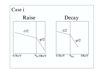
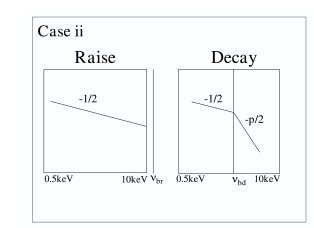
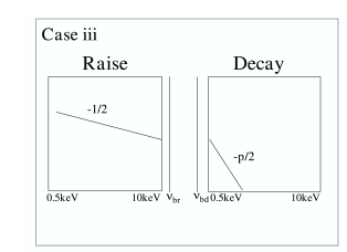
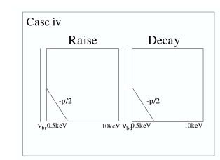
Figure 1: The four cases in the refreshed shock model explained in sec. 3.1

Figure 2: Power-law decay indices of the GRB050713A second flare light curves in the 0.3–0.8, 0.8–1.4, 1.4–2.2, 2.2–4, and 4–10 keV bands, starting from 108 s after $t_{0}$, as a function of the energy. The prediction of the synchrotron model is represented by the dashed lines, considering a broken power-law for two different values of $p$.

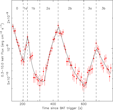
Figure 3: Swift XRT 0.3-10 keV light curve of the GRB 050730 X-ray afterglow during the first orbit. The solid line is the best fit model to the data obtained considering a linear rise exponential decay for the three flares (see Sect. LABEL:temporal of Perri et al. 2006). The dashed vertical lines delimit the seven time intervals considered for the spectral analysis. Data are binned to 8 seconds resolution and errors are at the 1$\sigma$ level.

3.2 Late internal shocks

($\Delta T<<T$ )

A diagnostic to check if the re-brightenings are due to late internal shocks has been recently proposed by Liang et al. 2006 [24]. In the internal-origin scenario for X–ray flares the decay emission of the flaring episodes should be dominated by high-latitude emission with the temporal decay index related to the decay spectral index as $\alpha_{\rm d}=\beta_{\rm d}+2$ ([25]). Liang et al. 2006 use the time integrated spectrum; however in order to test the curvature effect, the analysis should be done using the spectrum in the decay phase of the flare. We have checked this interpretation for the first three bright X–ray flares observed in GRB050730 afterglow shown in Fig.3 and we plan to extend the analysis to all flares in our sample [22]. We used the spectral indices measured during the decay and found best fit zero times [21] $t_{0,1}=77^{+22}_{-29}$ s, $t_{0,2}=234^{+52}_{-85}$ s and $t_{0,3}=174^{+99}_{-152}$ s, respectively. Comparing these values with the rise times given in Table 1, we can see that for all three episodes the zero time values are not located during the rising portion of the corresponding flare, clearly indicating that the observed decay slopes are not consistent with being due to high-latitude emission, as predicted by the late internal shock scenario.

Nonetheless there are flares that can be better explained with the internal shock model even if $\Delta T\sim T$. These are for example GRB050406 and GRB050502B where the presence of an underlying continuum in the X-ray lightcurve, consistent with the same slope before and after the flare argues against the external shock models in the adiabatic regime, since no trace of an energy injection can be found. However it is possible that for these flares the radiative regime applies [22]. If we consider $T_{0}=T_{\rm rise}$ we estimate $\alpha_{\rm d,IS}=-3.2\pm 0.7$, $\alpha_{\rm d,IS}=-4.3\pm 0.1$ and $\alpha_{\rm d,IS}=-1.4\pm 0.2$ for GRB050406, GRB050502B and GRB050822 (that is the only one that has $\Delta T<<T$). We can compare these values with the ones expected by the curvature effect. For GRB050406 we find $\alpha_{\rm d,IS}=-(\beta_{d}+2)=-3.2$, in agreement with the observed value, whereas for GRB050502B and GRB050822 we find $\alpha_{\rm d,IS}=-3.3$ and $\alpha_{d}=-3.8$, which are different from the observed values.

Table 2: Best fit values for the temporal and spectral power slopes. We also indicate which models best interprets the flares phenomenology, internal shocks (IS) and refreshed shocks (RS). For the RS model we also report to which case of the ones discussed in sec 3.1 the GRB belongs

GRB	$\alpha$	NH	$\Gamma$	$\chi^{2}_{\rm R}$	model
		$10^{22}$cm-2
050406(r)	$1.1\pm 0.4$	$<0.09$	2.45$\pm$0.71	0.6
050406(d)	$-1.05\pm 0.3$	$<0.06$	2.23$\pm$0.55	1.42	IS
050502B(r)	$1.41\pm 0.03$	0.15$\pm$0.01	2.27$\pm$0.03	1.02
050502B(d)	-0.88	0.08$\pm$0.01	2.33$\pm$0.04	1.2	IS
050713A(1r)	$0.67\pm 0.05$	$0.53\pm 0.09$	1.60 $\pm$ 0.15	1.11
050713A(1d)	-0.25 to -1	$0.62\pm 0.05$	2.60 $\pm$0.15	1.27	RS case i
050730(1r)	$0.37\pm 0.12$	$1.6^{+2.5}_{-1.6}$	1.29 $\pm$ 0.16	0.86
050730(1d)	$-0.41\pm 0.06$	$3.1^{+1.3}_{-1.1}$	1.82 $\pm$0.12	1.3
050730(2r)	$0.92\pm 0.10$	$2.1^{+0.8}_{-0.7}$	1.71 $\pm$ 0.08	1.1
050730(2d)	$-0.67\pm 0.16$	$0.9\pm 0.5$	1.70 $\pm$0.12	1.1	RS case iv
050730(3r)	$0.51\pm 0.12$	$0.7^{+0.8}_{-0.7}$	1.77 $\pm$ 0.12	0.87
050730(3d)	$-0.27\pm 0.08$	$1.0\pm 0.6$	2.01 $\pm$0.1	0.81
050822(r)	$0.45\pm 0.15$	0.24$\pm$0.05	2.8$\pm$0.2	0.8
050822(d)	$-0.56\pm 0.08$	0.19$\pm$0.04	2.8$\pm$0.2	0.9	IS
050904(r)	$0.25\pm 0.06$	0.14$\pm$0.02	1.76$\pm$0.06	1.22
050904(d)	-0.64$\pm$ 0.05	0.07$\pm$0.03	1.75$\pm$0.08	0.8	RS case iv
060111A(r)	0.000	0.14$\pm$0.02	1.76$\pm$0.06	1.22
060111A(d)	0.48$\pm$ 0.03	0.07$\pm$0.03	1.75$\pm$0.08	0.8	RS

Table 3: Broken power law fits for the spectra.

GRB	NH	$\Gamma_{2}$	Eb	$\chi^{2}_{\rm R}$
	$10^{22}$cm-2
050406(r)	na	na	na	na
050406(d)	na	na	na	na
050502B(r)	0.12$\pm$ 0.02	2.25$\pm$ 0.04	0.71$\pm$ 0.08	0.96
050502B(d)	0.04$\pm$ 0.02	2.29 $\pm$ 0.05	0.72$\pm$ 0.08	1.09
050713A(1r)	$0.50\pm 0.09$	$1.95^{+0.75}_{-0.35}$	$3.75^{+1.5}_{-1.75}$	1.18
050713A(1d)	$0.62\pm 0.05$	2.67 $\pm$ 0.17	$1.8\pm 0.2$	1.18
050730(1r)	$1.6^{+2.5}_{-1.6}$	1.29 $\pm$ 0.15	$<2.2$	0.89
050730(1d)	$2.0^{+1.1}_{-0.8}$	1.85 $\pm$ 0.12	$1.1^{+0.7}_{-0.3}$	1.28
050730(2r)	na	na	na	na
050730(2d)	na	na	na	na
050730(3r)	na	na	na	na
050730(3d)	na	na	na	na
050822(r)	0.2$\pm$ 0.1	2.8$\pm$ 0.3	0.7$\pm$ 0.3	0.7
050822(d)	na	na	na	na
050904(r)	0.13$\pm$ 0.04	1.73$\pm$ 0.07	0.7$\pm$ 0.6	1.2
050904(d)	0.06$\pm$ 0.05	1.74$\pm$ 0.09	0.8$\pm$ 0.7	0.8
060111A(r)	0.14$\pm$0.02	1.76$\pm$0.06	1.22
060111A(d)	0.06$\pm$ 0.05	1.74$\pm$ 0.09	0.8$\pm$ 0.7	0.8

4 Discussion

It is by now apparent that flares in the light curves of GRBs decay have different characteristics. While it may prove difficult to explain their complex phenomenology within the framework of a single model, we can nevertheless constrain some of the models by carefully exploiting the present data.

We have presented a timing and spectral analysis of several flares detected by Swift. Since the main energy output of the GRB engine rapidly decays with time [26], the energy injections are likely due either to slower shells ejected during the prompt phase of the GRB engine and catching up at later times (refreshed shocks), or to later energy production episodes in the central engine, due, e.g.,to disk fragments that accrete at later times [16] (late internal shocks). We have proposed a method to distinguish between these two different models based on the estimate of the flare duration and on the comparison between the spectral and temporal slopes.

We found that the flares of GRB050713A, GRB050730 and GRB050904 can be explained by the refreshed shock model. We saw that the flares in GRB050730 do not satisfy the relation implied by the curvature effect between the temporal and spectral slope, indicating that internal shocks may be less likely in this case. However there are other bursts (like GRB 050406, GRB 050502B and GRB050822) were late internal shocks may interpret better the flares characteristics. We plan to extend our analysis to a larger sample of Swift GRBs.

Flaring activity is also observed in the optical afterglow of some GRBs (like GRB 050730 see Perri et al. 2006). Detection of optical rebrightenings in the light curve would also help in testing the models. Simultaneous re-brightening events in the X–ray and optical bands, like the ones seen in GRB 050730 can be easily explained in the refreshed shock model (e.g. [27]).

This research has been partially supported by A SI grant I/R/039/04 and MIUR.

References

- [1] \BYLaursen L.T. \atqueStanek K.Z. \INAstrophys. J.5972003L107
- [2] \BYSari R., Piran T. \atqueNarayan R. \INAstrophys. J.4971998L17
- [3] \BYBersier D. et al. \INAstrophys. J.5842002L43
- [4] \BYMatheson T. et al. 2002 \INAstrophys. J.5822002L5
- [5] \BYGehrels N. et al \INAstrophys. J.6212005558
- [6] \BYBurrows D. N. et al. \INScience30920051833B
- [7] \BYFalcone A.D. et al. \INAstrophys. J.64120061010
- [8] \BYNousek J. A. et al. \INAstrophys. J.6422005389
- [9] \BYO’Brien P. T. et al. \INAstrophys. J.647200612130
- [10] \BYRomano P. et al. \INAstron. \atqueAstrophys.4562006917
- [11] \BYKobayashi S. et al. astro-ph/0506157
- [12] \BYLazzati D., et al. \INAstron. \atqueAstrophys.3962002L5
- [13] \BYZhang B. et al. \INAstrophys. J.6422006354
- [14] \BYKing A. et al. \INAstrophys. J.6302005L113
- [15] \BYMacFadyen A. I., Ramirez-Ruiz E. \atqueZhang W. astro-ph/0510192
- [16] \BYPerna R. Armitage P. J. \atqueZhang B. \INAstrophys. J.6362006L29
- [17] \BYGao W. H. \atqueFan Y.Z. astro-ph/0512646 submitted to ApJ
- [18] \BYProga D. \atqueZhang B. \INMNRAS370L61
- [19] \BYKumar P. \atquePiran T. \INAstrophys. J.5322000286
- [20] \BYGuetta D. et al. \INAstron. \atqueAstrophys.2006inpress
- [21] \BYPerri M. et al. \TITLEsubmitted to Astron. and Astrophys.
- [22] \BYGuetta D. et al. \TITLEin preparation
- [23] \BYCapalb M. et al. \TITLEThe SWIFT XRT Data Reduction Guide http://heasarc.gsfc.nasa.gov/docs/swift/analysis/xrt_swguide_v1_2.pdf
- [24] \BYLiang E.W. et al. \INAstrophys. J.6462006L351
- [25] \BYKumar P. \atquePanaitescu \INAstrophys. J.5412000L51
- [26] \BYJaniuk A., Perna R., Di Matteo T. \atqueCzerny B. \INMNRAS3552004950
- [27] \BYGranot J., Nakar E. \atquePiran T. \INNature4262003138
- [28] \BYChincarini G. et al in preparation