A gravitational wave window on extra dimensions

Abstract

We report on the possibility of detecting a submillimetre-sized extra dimension by observing gravitational waves (GWs) emitted by pointlike objects orbiting a braneworld black hole. Matter in the ‘visible’ universe can generate a discrete spectrum of high frequency GWs with amplitudes moderately weaker than the predictions of general relativity (GR), while GW signals generated by matter on a ‘shadow’ brane hidden in the bulk are potentially strong enough to be detected using current technology. We know of no other astrophysical phenomena that produces GWs with a similar spectrum, which stresses the need to develop detectors capable of measuring this high-frequency signature of large extra dimensions.

Motivation

String theory-inspired braneworld models Horava and Witten (1996); Randall and Sundrum (1999) envisage our universe as a 4D membrane embedded in some higher-dimensional space. Standard Model particles and fields are assumed to be confined to the ‘brane’, while gravity propagates in the higher-dimensional ‘bulk’. The principal observational features of such models take the form of modifications to 4D gravity. For static situations, we expect deviations from Newton’s law at distances less than the curvature scale of the bulk, $\ell$. Precision laboratory measurements yield that $\ell\lesssim 0.1\,\text{mm}$ Adelberger et al. (2003). Similarly, as we demonstrate here, in the case of dynamic gravitational fields we can expect significant higher-dimensional effects at frequencies in excess of $\sim c/\ell$. Presently, there is a vigorous worldwide effort to build detectors capable of observing dynamic gravitational degrees of freedom (i.e., gravitational waves) and hence verify one of the last untested predictions of Einstein’s general relativity. An intriguing question is how the braneworld paradigm may affect what these detectors see, and whether or not we can obtain useful constraints on extra dimensions. To address these issues, we need to concretely model how GWs are generated in braneworld scenarios. The purpose of this work is to predict the spectrum and amplitude of GWs generated by pointlike bodies orbiting a braneworld black hole.

The black string braneworld

As in our previous work with R. Maartens Seahra et al. (2005), we model a braneworld black hole as a 5D black string spacetime between a ‘visible’ brane at $y=0$ and a ‘shadow’ brane at $y=d$. The metric is given by $ds_{5}^{2}=e^{-2|y|/\ell}ds_{\text{Schw}}^{2}+dy^{2},$ where $ds_{\text{Schw}}^{2}$ is the 4D Schwarzschild line element. We require $d/\ell\gtrsim 5$ to comply with post-Newtonian solar system constraints Garriga and Tanaka (2000). This looks like the Schwarzschild solution on ‘our’ visible brane, with deviations from GR appearing perturbatively. This solution is stable if the mass of the string $M$ is large compared to the brane separation: ${M}/{M_{\odot}}\gtrsim 1.1\times 10^{-6}({\ell}/{0.1\,\text{mm}})\,e^{(d-5\ell)/\ell}$. If the string is too light an instability shows up in the spherical perturbations, but not for higher multipoles Gregory and Laflamme (1993); Kudoh (2006).

Kaluza-Klein radiation from orbiting particles

A small compact object (which we model as a delta function) of mass $M_{p}$ on either brane will orbit the black string in the same way as it would a Schwarzschild black hole in 4 dimensions. As in GR, it will emit massless spin-2 gravitational radiation, but unlike GR it will also generate fluctuations in the brane’s position as well ‘Kaluza-Klein’ (KK) modes. These are 5D massless GWs that have momentum along the extra dimension, and so behave like a coupled system of spin-0, spin-1, and spin-2 massive fields on either brane. Owing to the finite separation of the branes, the spectrum of KK masses $m_{n}$ is discrete. We concentrate on the spherical component of KK radiation generated by particles orbiting the string on either the visible or shadow brane.

As described in the Appendix, spherical KK modes are governed by a pair of one-dimensional coupled wave equations sourced by the particle. To illustrate typical waveforms seen by distant observers, we numerically integrate these equations in the case when the dimensionless KK mass is $\mu=GMm/\hbar c=0.5$. We consider two types of source trajectory: an eccentric periodic orbit (Fig. 1), and a ‘fly-by’ orbit (Fig. 2). In the former instance a nearly monochromatic steady-state signal is seen far from the string, while in the latter case we see a burst of radiation followed by a slowly decaying tail.

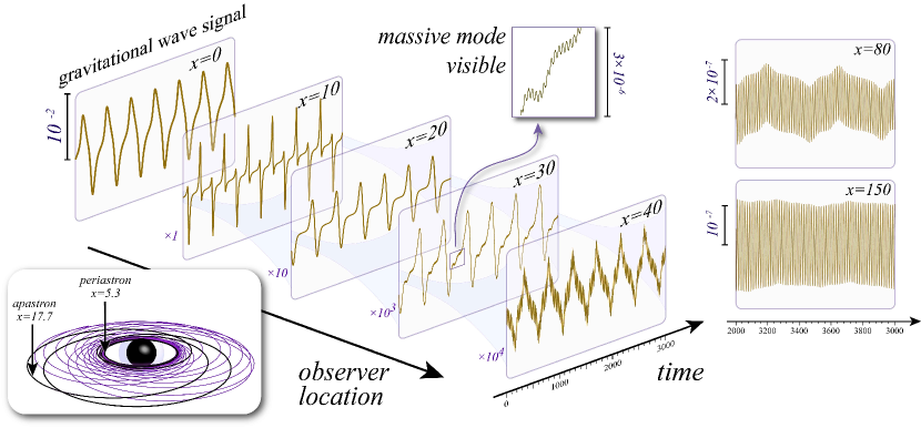
Figure 1: Radiation from a periodic orbit. The steady-state KK gravitational wave signal induced by a particle undergoing a periodic orbit around the black string with $\mu=0.5$. The orbit (bottom left) has eccentricity 0.5 and angular momentum 3.62 in the notation of Refs. Martel (2004); Cutler et al. (1994). The waveform of radiation falling into the black string is quite different than that of radiation escaping to infinity: The infalling signal precisely mimics the orbital profile of the source, while the outgoing signal is dominated by monochromatic radiation whose frequency is proportional to the KK mass $f=mc^{2}/2\pi\hbar$.

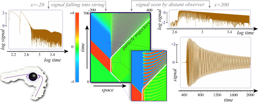
Figure 2: Radiation from a fly-by orbit The massive mode ($\mu=0.5$) GW signal from a fly-by orbit (bottom left) with eccentricity $3.0$ and angular momentum $\sim 3700$. We show the generated radiation in a spacetime diagram (center), as seen by an observer close to the string (top left), and as seen by a distant observer (right).

For a given source, it is possible to estimate the amplitude $h_{n}$ of each massive mode as measured on earth. We show these amplitudes as a function of their frequency $f_{n}$ in Fig. 3 for a number of different cases. Note that the KK frequencies are bounded from below: $f_{n}\geq f_{\text{min}}\sim 12\,\text{GHz}\left({\ell}/{0.1\,\text{mm}}\right)^{-1}e^{-(d-5\ell)/\ell}$. The variation of amplitude with frequency is qualitatively different for $f_{n}$ greater or less than a critical value: $f_{\text{crit}}={c}/{\pi^{2}\ell}\sim 304\,\text{GHz}\left({\ell}/{0.1\,\text{mm}}\right)^{-1}$. For ‘visible’ sources located on our brane, the amplitudes are peaked for $f_{n}\sim f_{\text{crit}}$. For ‘shadow’ sources located on the other brane, the $h_{n}$ are both independent of frequency and maximised for $f_{n}\lesssim f_{\text{crit}}$. In either case, the amplitudes are bounded from above $h_{n}\lesssim h_{\text{max}}$, where

$$h_{\text{max}}\sim\mathcal{A}\left(\frac{M_{p}}{M_{\odot}}\right)\left(\frac{r}{\text{kpc}}\right)^{-1}\left(\frac{M}{M_{\odot}}\right)^{-1/2}\left(\frac{\ell}{0.1\,\text{mm}}\right)^{1/2}\\ \times\begin{cases}5.0\times 10^{-22}e^{-(d-5\ell)/\ell},&\text{visible source},\\ 9.1\times 10^{-21}e^{-(d-5\ell)/2\ell},&\text{shadow source}.\end{cases}$$ (1)

Here, $r$ is the distance to the string and $\mathcal{A}$ is the characteristic signal amplitude determined from simulations. We find that $\mathcal{A}\sim 1$ for fly-by orbits and $\mathcal{A}\sim 10^{-6}$ for periodic orbits. In the former case, $h_{\text{max}}$ is comparable to the expected signal strength in GR.

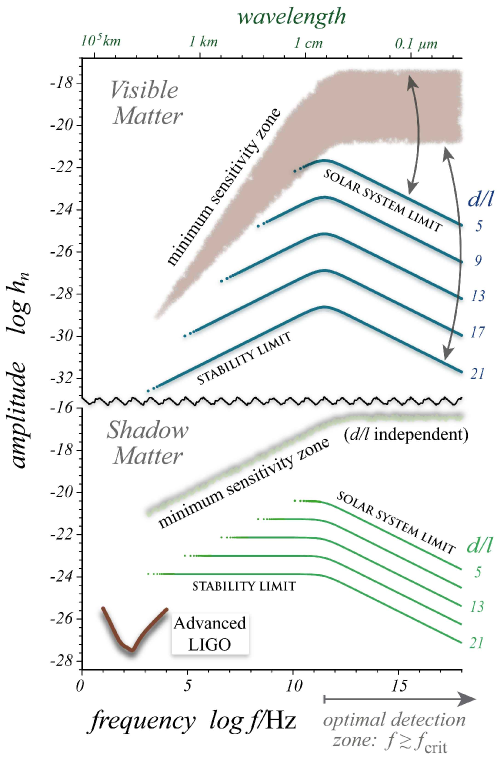
Figure 3: Massive mode amplitudes for visible and shadow sources. We have taken $\ell=0.1\,$mm, the string mass to be $10\,M_{\odot}$, the particle mass to be $1.4\,M_{\odot}$, source distance to be $1\,$kpc, and $\mathcal{A}=1$. For comparison, the dimensionless one-year sensitivity curve for Advanced LIGO (ALIGO) LIG is shown Arun et al. (2005). The shaded region shows the minimum $h_{\text{strain}}\,\text{Hz}^{1/2}$ required to detect the KK signal with $\text{SNR}\geq 5$ as a function of detector frequency $f_{0}$, assuming a one-year integration time and a periodic source.

Detection scenarios

Consider a GW detector whose sensitivity is characterised by the spectral noise density $S(f)$. If $H_{n}(t)$ is the detector’s (linear) response to the $n^{\text{th}}$ KK mode, then the signal-to-noise ratio for the total massive mode signal built-up over an observation time $T$ is $\text{SNR}=[\sum_{n}{2}{S^{-1}(f_{n})}\int_{0}^{T}H_{n}^{2}(t)\,dt]^{1/2}$ Jaranowski and Krolak (2000). Since the frequency separation $\sim f_{\text{crit}}e^{-d/\ell}$ between KK modes is small in most cases, this sum can approximated by an integral. This leads to the semi-empirical formula:

$$\text{SNR}\approx\Gamma e^{d/2\ell}h_{\text{max}}\begin{cases}0.45\,T^{1/2},&\text{periodic orbit},\!\!\!\\ 0.83\,T^{5/6}_{\text{str}}f_{\text{crit}}^{1/3},&\text{fly-by orbit},\end{cases}$$ (2)

where $T_{\text{str}}=2GM/c^{3}\approx 4.9(M/M_{\odot})\,\mu\text{s}$ is the characteristic timescale set by the string mass, which is typically much less than the observation time. The pre-factor depends on the detector, particle orbit, and source location:

$$\Gamma=\Gamma[S,d,\ell]=\left[\int_{32.4e^{-d/\ell}}^{\infty}\frac{Q(u)}{S(f_{\text{crit}}{u})}du\right]^{1/2},$$ (3)

where

$$\begin{array}[]{ccc}\hline\cr Q(u)&\text{periodic orbit}&\text{fly-by orbit}\\ \hline\cr\hline\cr\text{visible source}&2u(1+u^{2})^{-1}&2u^{5/3}(1+u^{2})^{-1}\\ \text{shadow source}&(1+u^{2})^{-1/2}&u^{2/3}(1+u^{2})^{-1/2}\\ \hline\cr\end{array}$$ (4)

Detectors which maximise $\Gamma$ stand the best chance of detecting the KK signal.

The simplest noise model for a GW detector is one in which the characteristic strain sensitivity $h_{\text{strain}}=\sqrt{S(f)}$ is constant over a band $[f_{0}-\Delta f,f_{0}+\Delta f]$, and is otherwise infinite. In Fig. 3, we show the $h_{\text{strain}}$ required of such a detector in order to observe periodic-orbit KK radiation as a function of $f_{0}$. We hold the logarithmic bandwidth of the detector constant, which yields that the minimum sensitivity is actually independent of $f_{0}$ for $f_{0}\gtrsim f_{\text{crit}}$. That is, the optimal means of detecting this type of KK radiation is via a high-frequency GW detector with $f_{0}\gtrsim f_{\text{crit}}$. Several designs for devices approaching this zone have been proposed or implemented Cruise (2000); Ballantini et al. (2003). Fig. 4 shows how such a detector can be used to constrain the fundamental parameters of our model.

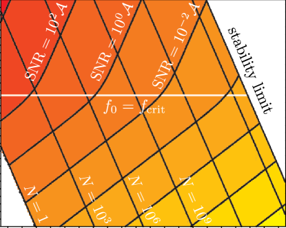
Figure 4: Observations in the extra-dimensional parameter space. Signal-to-noise prediction for massive mode GWs generated by a fly-by orbit on the visible brane for a high-frequency detector with $f_{0}=10^{14}\,\text{Hz}$, $\Delta f=10^{13}\,\text{Hz}$, and $h_{\text{strain}}=10^{-23}\,\text{Hz}^{-1/2}$. The particle mass is $1\,M_{\odot}$ while the string corresponds to the ‘black hole’ at the galactic centre ($M\approx 4\times 10^{6}\,M_{\odot}$ and $r\approx 8\,\text{kpc}$); the scaling of SNR with $M_{p}$ and $r$ is given by (1). Also shown are the number of KK modes $N$ in this detector’s range as a function of $\ell$ and $d/\ell$. Assuming that the other parameters can be obtained from other observations (e.g. the zero-mode GW signal), simultaneous measurements of SNR and $N$ can determine the bulk curvature scale and brane separation uniquely.

Eqs. (1) and (2) imply that the detector-independent ratio $\text{SNR}/\Gamma$ decreases exponentially with $d/\ell$ for visible matter, but is independent of brane separation for shadow matter. Furthermore, as seen in Fig. 3, the KK amplitudes $h_{n}$ generated by shadow matter are not suppressed for $f_{n}\lesssim f_{\text{crit}}$, unlike the visible matter case. These facts imply that a direct detection of shadow matter is within the capability of ‘low-frequency’ devices such as LIGO and ALIGO, which are otherwise insensitive to KK radiation from realistic sources on our brane. In Fig. 5, we show the types of events detectable by these two interferometers when they achieve their respective design sensitivities.

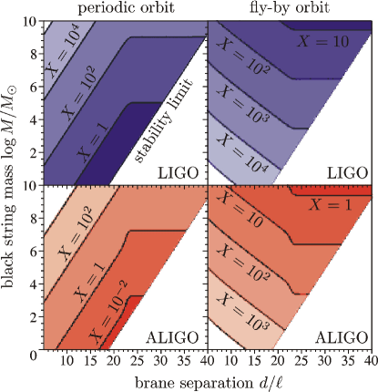
Figure 5: Prospects for detecting KK radiation from shadow matter particles by LIGO and ALIGO. For any black string-shadow particle interaction, we can assign a detectability statistic $X=\mathcal{A}(M_{p}/M_{\odot})(r/\text{kpc})^{-1}$. The contours indicate events that are detectable with $\text{SNR}\geq 1$ (assuming a one-year integration time in the case of periodic sources, and $\ell=0.1\,$mm). We have assumed that the detector sensitivity is entirely photon shot-noise/radiation pressure limited for $f\gtrsim 10^{4}\,\text{Hz}$.

Discussion

Gravitational waves may well prove to be a critical tool in placing limits on, or detecting positive signatures of, large extra dimensions. By using a simple model of a braneworld black hole, we have shown how brane-confined matter can generate GW signals with a characteristic frequency fixed by the curvature scale of the extra dimension—around $300\,$GHz or above—and with amplitude comparable to the predictions of GR. The most efficient (and cost-effective) means of observing KK radiation generated on our brane is with a high-frequency GW detector optimised for all spins of radiation. The detection of such a signal would provide a strong evidence in favour of new physics (such as a large extra dimension), since there are no astrophysical sources that can generate a similar spectrum of GWs. (Certain models of inflation can generate GWs with $f\sim 10^{12}\,\text{Hz}$ Giovannini (1999), but not with a discrete spectrum.)

It is remarkable that both the intrinsic strength and shape of the shadow matter GW spectrum implies that it is easier to detect than KK radiation from visible matter. In braneworld models, the only means of directly observing material hidden in the bulk is via gravitational interactions, so the search for KK radiation is one of the few viable techniques that can constrain the shadow brane’s matter content. Intriguingly, our work suggests that real observational constraints on shadow matter are within the grasp of current technology such as LIGO.

We note that the discrete frequencies within the KK spectrum are independent of the string and particle masses. That is, all such systems will generate GWs with the same frequencies, hence there will likely be a significant (non-cosmological) integrated stochastic GW background in this model. Indeed, one would expect such a background to be generated in any model incorporating ‘ultraviolet’ modifications to GR at length scales $\ell\lesssim 0.1\,$mm. Hence, stochastic GW backgrounds might prove to be a useful model-independent observational window onto submillimetre-scale exotic physics.

Finally, we reiterate that all of our results have been calculated using the delta-function approximation for brane sources. An important open issue involves the effects of more sophisticated source modeling, but this is left for future work.

Appendix

In the Randall-Sundrum gauge Randall and Sundrum (1999), perturbations of the black string metric are orthogonal to the extra dimension and given by $g_{\alpha\beta}\rightarrow g_{\alpha\beta}+\sum_{n=0}^{\infty}Z_{n}(y)h^{(n)}_{\alpha\beta}(x^{\mu})$. The linearized Einstein field equations yield that the $Z_{n}$ are eigenfunctions of $-e^{-2|y|/\ell}(\partial_{y}^{2}-4/\ell^{2})$ with discrete eigenvalues $m_{n}^{2}c^{2}/\hbar^{2}$, which are the effective masses of the KK gravitons $h_{\alpha\beta}^{(n)}$. The $n=0$ contribution is massless and hence reproduces ordinary GR. To avoid the Gregory-Laflamme instability, we need $\mu_{n}=GMm_{n}/\hbar c>0.4301$ for all $n>0$.

The individual components of the spherical part of $h_{\alpha\beta}^{(n)}$ can be derived from a master variable $\psi$, which satisfies

$$(\partial_{\tau}^{2}-\partial_{x}^{2}+V_{\psi})\psi = \mathcal{S}_{\psi}+\mathcal{{I}}\,\varphi,$$ (5a)

$$(\partial_{\tau}^{2}-\partial_{x}^{2}+V_{\varphi})\varphi = \mathcal{S}_{\varphi},$$ (5b)

where we have defined the dimensionless coordinates $\tau={tc^{3}}/{GM}$ and $x={rc^{2}}/{GM}+2\ln\left({rc^{2}}/{2GM}-1\right)$. The tortoise coordinate $x$ maps the event horizon at $r=2GM/c^{2}$ onto $x=-\infty$. In these wave equations, $\varphi$ is another master variable that governs spherical perturbations in the position of the brane on which the matter source resides. The equations are coupled by the interaction operator ${\mathcal{I}}={\mathcal{I}}(x,\partial_{x})$, and $V_{\psi,\phi}$ are potentials.

The source terms $\mathcal{S}_{\psi}$ and $\mathcal{S}_{\varphi}$ depend on the perturbing brane matter. As in GR, we analytically model a small brane particle using a stress-energy tensor with delta-function support along its worldline. In numeric simulations, the delta-functions are replaced with a narrow Gaussian profile Lopez-Aleman et al. (2003); Sopuerta et al. (2006). There are a few ambiguities in this regularization scheme, but we find that our numeric results far from the string are largely insensitive to the particular choices made.

A detailed analysis leads to the following late-time/distant-observer approximation for the KK metric perturbations:

$$\!\!\!h^{(n)}_{\alpha\beta} \approx h_{n}e^{i\omega_{n}t}\,\,\text{diag}\left(0,+1,-\tfrac{1}{2}r^{2},-\tfrac{1}{2}r^{2}\sin^{2}\theta\right)$$ (6)

$$\times\begin{cases}1,&\text{periodic orbits},\\ (tc^{3}/GM)^{-5/6},&\text{fly-by orbits},\end{cases}$$

where $|h_{n}|=\sqrt{8\pi}\mathcal{A}\left(\frac{2GM_{p}}{rc^{2}}\right)\left(\frac{2GM}{\ell c^{2}}\right)^{-1/2}F_{n}(d/\ell)$. $\mathcal{A}$ is a dimensionless quantity that depends on the particle orbit but not on any other parameters; its value must be determined from simulations. $F_{n}(d/\ell)$ is a complicated expression with the following limiting behaviour: When the perturbing matter is on our brane

$$F_{n}(d/\ell)\approx\begin{cases}\tfrac{1}{2}e^{-3d/2\ell}(n\pi^{3})^{1/2},&n\ll 2e^{d/\ell}/\pi^{2},\\ e^{-d/2\ell}(n\pi)^{-1/2},&n\gg 2e^{d/\ell}/\pi^{2}.\end{cases}$$ (7a)

On the other hand, for shadow particles

$$F_{n}(d/\ell)\approx\begin{cases}e^{-d/2\ell}(\pi/2)^{1/2},&n\ll 2e^{d/\ell}/\pi^{2},\\ (n\pi)^{-1/2},&n\gg 2e^{d/\ell}/\pi^{2}.\end{cases}$$ (7b)

Finally, to a good approximation, the KK frequencies are given by $\omega_{n}=2\pi f_{n}\approx\frac{c}{\ell}\left(n+\tfrac{1}{4}\right)\pi e^{-d/\ell}.$

References

- Horava and Witten (1996) P. Horava and E. Witten, Nucl. Phys. B475, 94 (1996).
- Randall and Sundrum (1999) L. Randall and R. Sundrum, Phys. Rev. Lett. 83, 3370 (1999).
- Adelberger et al. (2003) E. G. Adelberger, B. R. Heckel, and A. E. Nelson, Ann. Rev. Nucl. Part. Sci. 53, 77 (2003).
- Seahra et al. (2005) S. S. Seahra, C. Clarkson, and R. Maartens, Phys. Rev. Lett. 94, 121302 (2005).
- Garriga and Tanaka (2000) J. Garriga and T. Tanaka, Phys. Rev. Lett. 84, 2778 (2000).
- Gregory and Laflamme (1993) R. Gregory and R. Laflamme, Phys. Rev. Lett. 70, 2837 (1993).
- Kudoh (2006) H. Kudoh, Phys. Rev. D73, 104034 (2006).
- Martel (2004) K. Martel, Phys. Rev. D69, 044025 (2004).
- Cutler et al. (1994) C. Cutler, D. Kennefick, and E. Poisson, Phys. Rev. D50, 3816 (1994).
- (10) http://www.ligo.caltech.edu/.
- Arun et al. (2005) K. G. Arun, B. R. Iyer, B. S. Sathyaprakash, and P. A. Sundararajan, Phys. Rev. D71, 084008 (2005).
- Jaranowski and Krolak (2000) P. Jaranowski and A. Krolak, Phys. Rev. D61, 062001 (2000).
- Cruise (2000) A. M. Cruise, Class. Quant. Grav. 17, 2525 (2000).
- Ballantini et al. (2003) R. Ballantini et al., Class. Quant. Grav. 20, 3505 (2003).
- Giovannini (1999) M. Giovannini, Phys. Rev. D60, 123511 (1999).
- Lopez-Aleman et al. (2003) R. Lopez-Aleman, G. Khanna, and J. Pullin, Class. Quant. Grav. 20, 3259 (2003).
- Sopuerta et al. (2006) C. F. Sopuerta, P. Sun, P. Laguna, and J. Xu, Class. Quant. Grav. 23, 251 (2006).