Bar-Halo Friction in Galaxies III: Halo Density Changes

Abstract

The predicted central densities of dark matter halos in LCDM models exceed those observed in some galaxies. Weinberg & Katz argue that angular momentum transfer from a rotating bar in the baryonic disk can lower the halo density, but they also contend that $N$-body simulations of this process will not reveal the true continuum result unless many more than the usual numbers of particles are employed. Adopting their simplified model of a rotating rigid bar in a live halo, I have been unable to find any evidence to support their contention. I find that both the angular momentum transferred and the halo density change are independent of the number of particles over the range usually employed up to that advocated by these authors. I show that my results do not depend on any numerical parameters, and that field methods perform equally with grid methods. I also identify the reasons that the required particle number suggested by Weinberg & Katz is excessive. I further show that when countervailing compression by baryonic settling is ignored, moderate bars can reduce the mean density of the inner halo by 20% – 30%. Long, massive, skinny bars can reduce the mean inner density by a factor $\sim 10$. The largest density reductions are achieved at the expense of removing most of the angular momentum likely to reside in the baryonic component. Compression of the halo by baryonic settling must reduce, and may even overwhelm, the density reduction achievable by bar friction.

1. Introduction

The LCDM model for the formation of structure and galaxies in the universe makes specific predictions about the density profiles of galaxy halos. It is generally reported that the spherically averaged density profile approximates a broken power law of the form

$$\rho(r)={\rho_{s}r_{s}^{3}\over r^{\alpha}(r+r_{s})^{3-\alpha}},$$ (1)

with $\rho_{s}$ and $r_{s}$ setting the density and spatial scales, and $1\lesssim\alpha\lesssim 1.5$. The NFW profile (Navarro, Frenk & White 1997) has $\alpha=1$, but recent work supports larger values (e.g., Diemand et al. 2004). Power et al. (2003) and Navarro et al. (2004) suggest that the inner profile slope decreases continuously towards smaller radii, but the logarithmic slope remains $\lesssim-1$.

The halo concentration is defined as $c=r_{\rm out}/r_{s}$, with the outer radius, $r_{\rm out}$, being that inside of which the mean density, in units of the cosmic closure density, is $\bar{\delta}_{\rm out}$; commonly $\bar{\delta}_{\rm out}=200$. The concentration, $c$, can readily be related to $\rho_{s}$ by integrating eq. (1). Its mean value, which varies slowly with halo mass, is a second major prediction of the simulations (e.g., Bullock et al. 2001, but see also Neto et al. 2007).

Attempts to estimate the dark matter density profiles in galaxies directly are beset by many observational and modeling difficulties (e.g., Swaters et al. 2003; Rhee et al. 2004; Valenzuela et al. 2007). Alam, Bullock & Weinberg (2002) therefore proposed a quantity that is less sensitive to observational uncertainty, though still based on the spherically averaged mass distribution. They define $\Delta_{v/2}$ to be the mean halo density, normalized by the cosmic closure density, interior to the radius at which the circular speed of the halo alone rises to half its maximum value. As this radius is typically a few kiloparsecs from the center of a galaxy, the quantity is less sensitive to observational, or numerical, uncertainties. The quantity is easily extracted from simulations, and can be estimated from high-quality observational data, if the baryonic contribution to the central attraction is known, or can be neglected.

Figure 1.— After Alam et al. (2002). Solid and dashed lines show $\Delta_{v/2}$ predicted from two different parameter sets for LCDM and for two different values of the slope of the inner density profile. The error bar indicates the approximate spread in these predicted values. Plus symbols show the galaxy data collated by Alam et al., and the sources for the five large labeled points are described in the text.

A major advantage of $\Delta_{v/2}$ is that it does not require any assumption to be made about the halo density profile. However, it may be useful to note that for the NFW halo, $\alpha=1$ in eq. (1), we have $r_{v/2}\simeq 0.127r_{s}$, and $\hbox{$\Delta_{v/2}$}=3.36\bar{\delta}_{\rm out}c^{3}/[\ln(1+c)-c/(1+c)]$.

I have redrawn the principal figure of Alam et al. as Figure 1. The plus symbols show the points collated by those authors from fits to galaxies for which the baryonic contribution was assumed to be negligible. The points for NGC 4123 and NGC 3095 are from Weiner (2004), while that for NGC 1356 is from Zánmar Sánchez et al. (2008) using the same method. I plot two points for the Milky Way: the upper point is model B₁ from Klypin, Zhao & Somerville (2002), while the lower shows the upper limit from Binney & Evans (2001) that the maximum halo contribution at the solar circle ($r=8\;$kpc) is $100\hbox{ km s}^{-1}$. For this latter model, I adopted $v_{\rm max}=200\hbox{ km s}^{-1}$ in the Milky Way for the abscissa, but the ordinate does not depend on this assumption, since Binney & Evans argue that the halo density cannot increase steeply towards the center. It is unclear how these two separate models could be reconciled.

Predictions from two separate LCDM models are also reproduced from Alam et al. The solid lines in Fig. 1 show the predicted values of $\Delta_{v/2}$ when $\Omega_{m}=0.3$, $h=0.7$, $\sigma_{8}=1$, $n=1$, and for values of $\alpha=1$ & 1.5. The error bar indicates their estimated factor $\sim 2.5$ spread in the predicted values of $\Delta_{v/2}$. The recent WMAP results (Spergel et al. 2007) require a lower $\sigma_{8}$ and also suggest that the initial power spectrum of density fluctuations is not scale free, as assumed for the solid lines, but may be tilted with less power on small scales. Zentner & Bullock (2002) have already shown that power spectra of this form lead to halos of lower concentration, and the predictions for one such model ($\Omega_{m}=0.4$, $h=0.65$, $\sigma_{8}=0.7$ and $n=0.93$) adopted by Alam et al. are shown by the dashed lines. Modern data (e.g., Tegmark et al. 2006) indicate a slightly higher $\sigma_{8}$, suggesting that the dashed lines are on the low side.

The data points in this plot are not in good agreement with the predictions, especially since simulations suggest $\alpha>1$. Note that three of the large points, which are based on detailed models for each galaxy, are among the most discrepant, and that the discrepancy for these baryon-dominated galaxies will widen by at least a factor of a few when halo compression by baryonic infall is taken into account. The particular tilted spectrum model shown by the dashed lines reduces the discrepancy between the prediction and the data, but does not eliminate it. Dynamical friction constraints from Debattista & Sellwood (2000) lend support for low dark matter densities in barred galaxies.

The point for NGC 1365 is from an NFW halo with concentration $c_{200}=61$, which Zánmar Sánchez et al. (2008) determined to yield the best-fit to their data. I plot this point from the current compressed halo in order to be consistent with the other points that also show the compressed halos. Zánmar Sánchez et al. estimate that an initial halo with $c_{200}=22$ would yield an acceptable fit after compression, although the baryon fraction in this case is a very high 27%. This uncompressed halo is much closer to the LCDM predictions, and has $\hbox{$\Delta_{v/2}$}=3.5\times 10^{6}$, but most discrepancies would worsen were halo compression taken into account for all other galaxies also.

Low central densities of DM in galaxies today need not be a problem for LCDM if the cusps can be erased subsequently during galaxy formation or evolution. Several ideas to reduce the central DM density have been proposed:

• Binney, Gerhard & Silk (2001), and others have proposed that the halo profile is altered by adiabatic compression as the gas cools followed by impulsive outflow of a large fraction of the baryon mass. One possible mechanism to produce such an outflow might be supernovae and stellar winds resulting from a burst of star formation. The idea was examined by Navarro, Eke & Frenk (1997) and by Gnedin & Zhao (2002), who found that only a mild reduction in the central DM density could be achieved in this way. Gnedin & Zhao tested the extreme case that 100% of the baryonic component was somehow blasted out instantaneously, yet found that even with this deliberately extreme assumption, the central density decreased by little more than a factor of two, unless the initial baryons were unrealistically concentrated to the halo center.

• El-Zant, Shlosman & Hoffman (2001) propose that the cusp in the halo density can be erased by dynamical friction with orbiting mass clumps. In essence, this is a process of mass segregation, in which heavy “gas” particles lose energy and settle to the center due to interactions with the light DM particles. However, Jardel & Sellwood (2008) show that the settling time is uninterestingly slow unless the baryonic clumps are extremely massive.

• Milosavljević et al. (2002) point out that a binary supermassive black hole (BH) pair created from the merger of two smaller galaxies will eject DM (and stars) from the center of the merger remnant. They also argue that the DM mass removed for a given final BH mass is greater if the final BH is built up in a series of mergers each having correspondingly lower mass BHs. While this mechanism must operate wherever binary BHs have been formed, the radial extent over which the mass is reduced is rather limited. They predict that the cores in the DM halos could possibly be larger than those in the bulge stars, whereas the discrepancy shown in Fig. 1 applies to much larger radii. Furthermore, shallow density gradients are observed in DM-dominated galaxies with insignificant bulges (Simon et al. 2005; Kuzio de Naray et al. 2006) which are likely to have very low-mass BHs (Gebhardt et al. 2000; Ferrarese & Merritt 2000), if they contain BHs at all.

• Weinberg & Katz (2002) suggest that a bar in the disk could flatten the cusp also through dynamical friction. Here I study this possibility in more detail.

Bar-driven halo density changes in fully self-consistent simulations reported so far have been minor, and of both signs. Debattista & Sellwood (2000) showed a modest halo density reduction in their Fig. 2, and Athanassoula’s (2003) simulations also indicate a small halo density decrease. On the other hand, Sellwood (2003) and Colín, Valenzuela & Klypin (2006) report the opposite behavior in simulations with more extensive halos, finding instead that loss of angular momentum from the disk caused the halo to contract, with the deeper disk potential well compressing the halo still more. Holley-Bockelmann, Weinberg & Katz (2005) however, report that the inner cusp was flattened in most of their experiments. While the radial extent of the effect was modest, the cusp was erased to a radius less than one fifth the bar semi-major axis, they continue to insist that the effect can be important. They further argue that the absence of significant density reductions in some published cases is due to numerical inadequacies.

Thus two separate issues need to be clarified. First, what are the numerical requirements to obtain reliable results from simulations? and second, what physical properties of the bar affect the extent to which the halo density can be reduced?

Weinberg & Katz (2007a & b; hereafter WK07a and WK07b) claim that simulated halos should contain between tens of millions and billions of particles to obtain the correct result. They reach this conclusion from perturbative calculations of the interaction between a rotating quadrupole potential and orbits in a spherical halo. Previous theory (Tremaine & Weinberg 1984) had shown that the important exchanges occur at resonances, and while an individual halo orbit may either gain or lose angular momentum, a net torque arises because there is a slight excess of gainers over losers. WK07a argue that it is important to have an adequate density of particles in phase space in order to obtain the correct balance, a criterion they dub “coverage.” They also argue that density fluctuations due to a finite number of particles cause the orbits of particles in simulations to deviate from those in a smooth potential, and that particles will therefore diffuse into and out of resonances due to such effects. If the diffusion rate is high, the simulation will not capture the appropriate smooth behavior, affecting the torque between the bar and the halo particles. They further argue that the lumpiness of the potential due to particle fluctuations depends on the method for calculating the gravitational field, and that field methods that employ an expansion in a set of basis functions will be intrinsically smoother than all other methods, and will therefore yield more reliable results.

Studies of bar-halo interactions, the slowing of bars, and the evolution of halo mass profiles cannot be pursued with confidence until the issues raised by WK07a are addressed. It is important to check whether results from previous and future studies with the usual ${\cal O}(10^{6})$ particles are, or are not, compromised by numerical inadequacies.

In Paper I (Sellwood 2006), I demonstrated explicitly that resonant exchanges between halo particles and the quadrupole field of a mild bar were taking place. I also showed that simulations both with and without self-gravity could converge to a frictional drag that was independent of the number of particles for feasible particle numbers. The mild bars used in that study did not, however, cause any significant change to the halo mass profile and did not, therefore, represent a direct challenge to the claims by WK07a. Other studies (Athanassoula 2002; Ceverino & Klypin 2007) have demonstrated the existence of many orbits trapped in various resonances, suggesting that particle noise does not preclude trapping from occurring, even when $N\sim 10^{6}$.

In this paper, I first present (§3) a further study of bar-halo interactions with much stronger bars that do cause large density reductions in order to provide a direct test of the issues raised by WK07a. Again I find (§4) that numerical results are quite insensitive to the particle number and calculation method. As my results are at variance with the conclusions in WK07a & WK07b, I show (§5) that my simulations do indeed reproduce a strong resonant response. I also identify (§6) the reasons why those authors reached incorrect criteria for the number of particles needed.

I turn to the physically more interesting question of how strong and large a bar is needed to cause a large density reduction in the inner halo in §7. I show that large, massive, skinny bars can indeed flatten the central cusp, as was already reported by Hernquist & Weinberg (1992), and confirmed in the rigid bar experiments of Weinberg & Katz (2002), Sellwood (2003), and McMillan & Dehnen (2005). However, I also find that more realistic bars cause only slight density reductions. In §8, I show that the possible changes in $\Delta_{v/2}$ in real galaxies are limited by the angular momentum content of the baryons.

2. Model set up

In this section, I describe the numerical model I use throughout the paper. I choose a sufficiently simple model that others can easily check my experiments.

2.1. Halo

For the unperturbed halo I employ the Hernquist (1990) profile

$$\rho_{0}(r)={Mr_{s}\over 2\pi r(r_{s}+r)^{3}},$$ (2)

which has total mass $M$ and scale radius $r_{s}$. I use the isotropic distribution function (DF) for this halo, which is also given by Hernquist. The density declines as $r^{-1}$ for $r\ll r_{s}$ and as $r^{-4}$ for $r\gg r_{s}$. It should be noted that this model differs only in the outer power law slope from the Navarro, Frenk & White (1997) profile used by WK07b, but the important inner cusp is the same.

While all halo particles have equal mass in most cases, I also report experiments in which the particles have individual masses in order to concentrate greater numbers in the dense inner regions. I set particle masses proportional to a weight function $w(L)=L_{0}+L$, where $L=|\;\kern-2.5pt\hbox{$\mit L$}\kern-6.25002pt\kern 0.50003pt\hbox{$\mit L$}\kern-6.25002pt\kern-0.24994pt\raise 0.43304pt\hbox{$\mit L$}|$ is the total specific angular momentum in units of $(GMr_{s})^{1/2}$ and $L_{0}$ is a constant, and select particles from the DF weighted by $w^{-1}$. Figure 2 plots the boost factor for the effective number of particles $\eta(r)={\cal N}(r)/{\cal M}(r)$, where ${\cal N}(r)$ and ${\cal M}(r)$ are respectively the fraction of the number of particles and the fraction of mass enclosed within radius $r$.

Figure 2.— The radial variation of the boost factor to the effective number of particles when unequal particle masses are used. The solid line is for $L_{0}=0.01$ and the dashed line for $L_{0}=10^{-8}$.

Choosing $L_{0}=0.01$ results in the heaviest particle being some 250 times the mass of the lightest and in half the particles being enclosed in a sphere $r=0.6$. A smaller sphere with $r=0.33$ encloses the same fraction when $L_{0}=10^{-8}$, where the lightest particle is $4\times 10^{-9}$ of the mass of the heaviest. As the $N$-body codes used here are designed to simulate collisionless dynamics, a range of particle masses should not lead to any mass segregation. A test, run for 100 dynamical times with no perturbation, revealed no tendency for the small changes to either the specific energy or specific angular momentum of the particles to correlate with particle masses.

It is inefficient to employ many particles at large radii that take no part in the friction process. I therefore truncate the model by setting the DF to zero for all $E>\Phi(r_{\rm cut})$, with $\Phi(r)=-GM/(r+r_{s})$ being the gravitational potential of the infinite Hernquist halo. This change eliminates any particle with sufficient energy to reach $r>r_{\rm cut}$, and the density tapers smoothly to zero at $r=r_{\rm cut}$. The gravitational potential from the remaining particles is somewhat modified, and the model is no longer an exact self-consistent equilibrium. However, the results presented below show that the truncation has very little effect on the equilibrium and the density profile hardly evolves in response. I choose $r_{\rm cut}=15r_{s}$, while the bars I employ are typically much smaller, with semi-major axis $a\leq r_{s}$. I show in §4 that the density changes in the inner halo are unaffected by the choice of $r_{\rm cut}$ over a wide range of values.

2.2. Bar

In order to be able to control the bar parameters, I again employ artificial, rigid bars (see Paper I). The homogeneous ellipsoid has mass $M_{b}$ and axes $a:b:c$ with $a\geq b\geq c$. It is centered on the halo center, and rotates about its shortest axis at angular rate $\Omega_{b}$. The angular speed of the bar is adjusted to take account of the torque from the halo, assuming it slows as a rigid bar of moment of inertia $I=M_{b}(a^{2}+b^{2})/5$. I use only the (2,2) quadrupole term of the gravitational field of the bar, as originally proposed by Hernquist & Weinberg (1992). I have shown in Paper I that higher terms have a small effect, and suppression of the monopole terms allows the bar to be introduced without affecting the radial balance of the halo.

Table 1Values of $\alpha_{2}$ and $\beta_{2}$

$a/b$	$b/a$	$\alpha_{2}$	$\beta_{2}$
6.667	0.1500	17.9874	0.3822
6.000	0.1667	14.9372	0.3962
5.000	0.2000	10.6953	0.4225
4.545	0.2200	08.9196	0.4374
4.000	0.2500	06.9336	0.4586
3.571	0.2800	05.4966	0.4787
3.333	0.3000	04.7499	0.4917
3.226	0.3100	04.4255	0.4980
3.125	0.3200	04.1290	0.5043
3.000	0.3333	03.7717	0.5125
2.000	0.5000	01.3772	0.6059

The approximate quadrupole field adopted by Weinberg (1985) was designed to match that of a homogeneous bar. I write his expression for the bar quadrupole in spherical (not cylindrical, as mis-stated in Sellwood 2003) polar coordinates as

$$\Phi_{\rm b}(r,\theta,\phi)=-{GM_{b}\over a^{3}}{\alpha_{2}r^{2}\over 1+(r/a\beta_{2})^{5}}\sin^{2}\theta e^{2i(\phi-\phi_{0})},$$ (3)

where $a$ is the semi-major axis of the bar and $\phi_{0}$ is the phase angle of the bar major axis. I give Weinberg’s prescription for selecting the dimensionless amplitude and radius scaling parameters, $\alpha_{2}$ and $\beta_{2}$ in the Appendix and, for fixed $a/c=10$, list their values for the bars used here in Table 1.

I show, also in the Appendix, that this expression is a good match to the quadrupole field of a homogeneous bar when $a/b\approx 2$, but it gives a peak perturbation that is increasingly too strong as $a/b$ is increased. In Paper I, I used the exact quadrupole field, which I added to my numerical solution for the self-consistent part of the halo field. As expansion of the gravitational field in multipoles on spherical shells is not a widely used technique, such a bar field is hard for others to reproduce. Reproducibility therefore dictates that I use the simple and convenient expression (3), but it must be borne in mind that the density distribution corresponding to this quadrupole is increasingly different from that of a homogeneous ellipsoid having the nominal axis ratio as $a/b$ is increased.

As noted above, a fixed bar field is required in order to be able to control the properties of the bar and address the scientific objectives of this paper. Bars in real galaxies do not approximate homogeneous ellipsoids, but the quadrupole part of the field is unlikely to differ substantially from the form (3), which Weinberg (1985) selected in order to have the appropriate asymptotic behavior both for $r\ll a$ and for $r\gg a$. Few real bars have isophotes skinnier than $a/b\sim 3$ (Reese et al. 2007; Marinova & Jogee 2007), while their mass distributions are more concentrated than a uniform density, implying that the quadrupole field for a given $a/b$ probably peaks interior to $r/a=(2/3)^{1/5}\beta_{2}$, where the peak of the radial part of (3) occurs. Higher multipoles are considerably less important to the dynamics discussed here (Paper I). The monopole part of the bar field could be considered part of the spherical halo, although the orbits of the particles would be rather different. The two most significant approximations of the adopted bar field are that it slows as a rigid object and does not adjust in response to the loss of angular momentum from the bar.

I introduce the bar perturbation smoothly by increasing the quadrupole term as a cubic function of time from zero at $t=0$ to its final value at $t=t_{g}$. Tests revealed that the outcome was insensitive to the growth-time of the bar over a broad range of values, so all experiments reported here use $t_{g}=10$ in units in which $G=M=r_{s}=1$.

2.3. Determination of the gravitational field

In most calculations, I compute the gravitational field of the halo particles using the radial grid method originally devised by McGlynn (1984) with some refinements described in Sellwood (2003). The coefficients of a multipole expansion of the interior and exterior masses are tabulated at a set of radii. The default grid spacing for these experiments places the $j$th grid shell according to the rule $r_{j}=e^{\gamma j}-1$ with $\gamma=\ln(r_{\rm max}+1)/n$, where $n$ is the number of radial shells and $r_{\rm max}$ is the outer limit of the grid. I generally use $n=300$ radial grid shells, set $r_{\rm max}=16r_{s}$, and expand up to $l_{\rm max}=4$.

This default rule for the radial grid is arbitrary, however, and I also present results using the alternative rule $r_{j}=r_{\rm max}(j/n)^{2}$ in order to place grid points more densely in the inner parts. In this case, I have employed $n=1000$ radial shells.

In order to test the assertion by WK07b that field methods are superior to all others, I present some results using the self-consistent field (SCF) method described by Hernquist & Ostriker (1992), for which the fundamental function of the expansion is the Hernquist density function (eq. 2). With this procedure, I include 20 radial functions, while again expanding in angle up to $l_{\rm max}=4$.

Expansion to low azimuthal order in both methods eliminates small-scale variations of both the azimuthal and radial fields, thereby hiding the graininess of the particle distribution. Therefore, no further smoothing, such as gravity softening, is required for either method.

2.4. Lop-sided instability

I compute the motion of the halo particles in the gravitational field arising from the particles, together with that of the external field of the bar. Past experience (Sellwood 2003; McMillan & Dehnen 2005; WK07a) has revealed that a rigid bar can drive the center of the particle distribution away from the bar center, which results in unphysical evolution. Special precautions are therefore needed to keep the particle distribution centered on the bar. Since I compute the field of the halo particles by a surface harmonic expansion on spherical shells, it is simplest to eliminate only the $l=1$ terms from the field determination, which is sufficient to ensure that the distribution of forces is always point symmetric about the origin and no lop-sidedness can develop.

WK07b, who employ an SCF-type method, keep the $l=1$ term active but include the unchanging monopole term of the bar in order to inhibit growing asymmetries in the particle distribution, as did McMillan & Dehnen (2005) in some of their experiments. Not only does this stratagem complicate the creation of the initial equilibrium, it also introduces a rigid mass component that inhibits the collective effects responsible for cusp flattening. Furthermore, WK07b report that their results are unaffected by the omission or inclusion of the $l=1$ terms; eliminating the dipole contribution to self-gravity is therefore the simplest way to suppress this artifact. (This stratagem is easy with a field or grid method, but not for a tree code. McMillan & Dehnen describe how a tree code needs to be adapted in order to prevent unphysical behavior when rigid bars are employed.)

2.5. Other details

Unless otherwise stated, the simulations reported here employ $10^{6}$ equal mass particles that move with a basic time step of $0.005(r_{s}^{3}/GM)^{1/2}$, the radial grid has 300 spherical shells, and I expand the density distribution of the particles using only the $0\leq l\leq 4$ terms, with the $l=1$ term suppressed. These choices of parameters are justified in § 4.

As the orbital frequencies of particles decrease strongly with increasing radius, I employ the multi-zone time step scheme descibed in Sellwood (1985). I use 5 time-step zones with the step size increasing by a factor 2 from zone to zone; i.e. the outermost particles are stepped forward once for every 16 steps taken by the innermost particles. The contributions to the gravitational field from slowly moving particles are interpolated in time as needed when accelerating particles in the inner zones.

I adopt units such that $G=M=r_{s}=1$.

In order to estimate the halo mass profile at any time, I sort the particles in radius and record the radius of every $n$th particle. An estimate of the density is the mass of the $n$ particles between these two radii, divided by the volume of the spherical shell containing them, and I assign this value to be the density at the mid-point of that radial range. I reduce the noise in this estimate by combining multiples of $n$ particles over the bulk of the model.

Figure 3.— The time evolution of (a) the bar pattern speed and (b) the radii containing different mass fractions in the fiducial run. The smallest radius is that containing 200 particles, or $1/5\,000$th of the mass in particles, and the mass fraction is successively doubled for each subsequent trace. The initial and final density, (c), and mass, (d), profiles in the same run; the solid lines are measured from the particles while the dashed lines show the theoretical profile (2). Note that the decreased innner density requires that the mass enclosed (d) cannot meet up with the unperturbed mass profile until a larger radius than where the cusp in (c) is flattened.

3. A Fiducial Model

Following WK07b, I first present a fiducial model in which the bar has a semi-major axis $a=r_{s}$, a mass of half that of the halo enclosed within $a$ so that $M_{b}=0.125M$, and the initial pattern speed is set to place corotation at the bar end, i.e. $\Omega_{b}=0.5$ with the initial bar rotation period $=4\pi$ time units. The nominal axis ratio is $a:b:c=1:0.2:0.1$, although the actual quadrupole field employed in the simulation is stronger than that of this ellipsoid (see Appendix). Thus the bar is unrealistically large, massive, and skinny, but it makes a useful starting point since WK07b correctly argue such a model should be very easy to simulate.

The time evolution of the model is shown in Figure 3. Friction with the halo particles, which results from resonant interactions as described in Paper I and § 5 below, causes the pattern speed (Fig. 3a) to start to decrease as the perturbation amplitude grows. The bar amplitude reaches its final value at $t=10$; the bar pattern speed is dropping very rapidly at this time, but levels out later to about 25% of its initial value.

The halo mass profile (Fig. 3b) does not change at first, confirming that the model is an excellent initial equilibrium, despite the truncation at $r_{\rm cut}$. However, the central density undergoes a rapid decrease over the time interval $8\lesssim t\lesssim 12$, after which further changes are comparatively minor. Continuation of the evolution beyond $t=20$ revealed little further change, and it is therefore reasonable to describe the simulation at $t=20$ as representing its final state.

Fig. 3(c) shows the initial and final density profiles. As estimates of density from the finite number of particles always suffer from some noise, I plot the much more robust measure of the mass enclosed as a function of radius in Fig. 3(d). Initially, $M(r)\propto r^{2}$ in the cusp, while the almost homogeneous core at later times has $M(r)\propto r^{3}$ in the inner parts. These curves are measured directly from the radial distribution of particles with no smoothing, indicating that the monopole part of the potential derived from the particles cannot suffer from significant fluctuations.

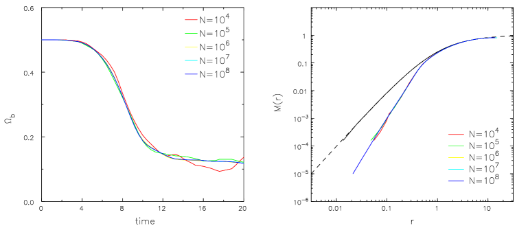
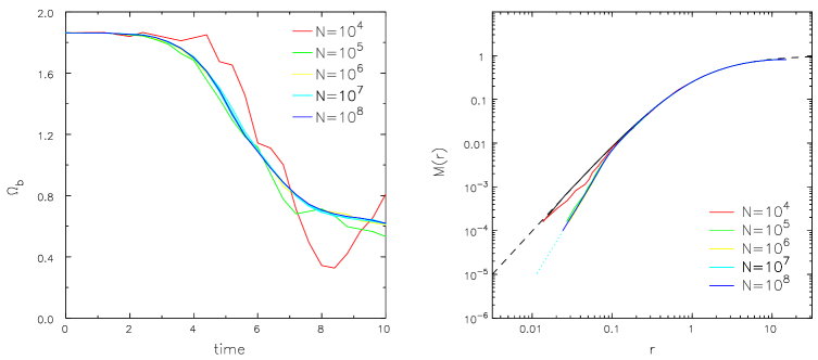
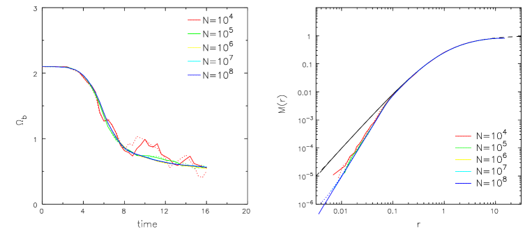
Figure 4.— The pattern speed evolution, left-hand panels, and initial and final mass profiles, right-hand panels, in three series of simulations in which the number of particles is varied. The top two rows show results using a grid method only and mostly equal mass particles. The bar length used in top panels is $a=r_{s}$ and in the middle panels $a=r_{s}/5$. The dotted curves in the middle panels show a results with $10^{7}$ unequal mass particles. The bottom panels are all for unequal mass particles and a still shorter bar with $a=r_{s}/6$; solid curves show results with a grid method, while dotted curves were obtained using a field method.

It should be noted that the density change shown in Fig. 3(c) is larger than that reported by WK07b in a similar experiment. As my result agrees with those found earlier (Hernquist & Weinberg 1992; Weinberg & Katz 2002; Sellwood 2003; McMillan & Dehnen 2005) and with those from other experiments with the NFW mass profile (not reported here), other differences in their physical model, such as the rigid monopole term, are the likely cause.

4. Numerical checks

Here I present a number of checks of this and other results that are designed to address some of the numerical concerns raised by WK07a and WK07b. In all cases, the bar mass is set to be half the enclosed halo mass at $r=a$, i.e. $M_{b}=0.5Ma^{2}/(r_{s}+a)^{2}$, and the initial pattern speed places corotation at the bar end, i.e. $\Omega_{b}=(GM/a)^{1/2}/(r_{s}+a)$.

4.1. Particle number

Figure 4 presents results from two series of experiments in which the number of equal-mass particles is varied over the range $10^{4}\leq N\leq 1.6\times 10^{8}$ for (top row) a large bar ($a=r_{s}$) and (middle row) a short bar ($a=r_{s}/5$). The evolution of the bar pattern speed and change in the mass profile are insensitive to the particle number as long as $N\gtrsim 10^{5}$; $N=10^{4}$ even seems adequate for the larger bar – the mass profile is less smooth but the reduction in density clearly does not differ significantly. It is worth noting that WK07b estimate that the large bar case requires $10^{8}$ equal-mass particles to obtain the appropriate behavior, whereas my result with $N>10^{8}$ is no different from that with three orders of magnitude fewer.

The convergence in Fig. 4 is exquisite; the different curves show direct measurements from the simulations without smoothing. Yet curves for the largest $N$ mostly overlay, and therefore obscure, those for the next largest $N$, and differences become visible only for much smaller $N$. WK07a correctly argue that if the phase space coverage were inadequate, exchanges at resonances would depend upon the few particles that happened to occupy the resonance, making the net balance between gainers and losers stochastic, and the resulting evolution could not converge as impressively as shown in Fig. 4. Repeated calculations of the large bar case with different random seeds reveal some slight stochastic behavior when $N=10^{4}$, but the evolution of the pattern speed and change to the mass profile is practically identical in another set of runs with $N=10^{6}$, as should be expected from the impressive data in Fig. 4.

The dotted curves in the middle row are from a run with unequal mass particles ($L_{0}=10^{-8}$), the alternative grid spacing rule and half the standard time step. The larger number of particles near the center allows the mass profile to be traced to smaller radii, but otherwise these refinements have no effect on either the pattern speed or mass profile evolution.

The bottom row of Fig. 4 is for a still shorter bar, this time with unequal mass particles selected with $L_{0}=0.01$ (see §2.1) and with a slightly rounder bar ($a/b=4$). The results shown by the solid curves were obtained using a grid method, while the dotted curves were obtained using the SCF method. The results from the two methods can barely be distinguished in most cases. It is clear that using unequal mass particles leads to convergence at a smaller $N$ in this numerically still more challenging case compared with that shown in the middle row.

WK07b report results from two experiments with $a=r_{s}/6$ that are similar to those in the bottom row of Fig. 4. Using unequal mass particles, they find a greater density reduction with $N=5\times 10^{6}$ than with $N=10^{6}$, which they attribute to the improved numerical quality of the slightly larger $N$ experiment. My experiments are not an exact match to theirs; the most important difference is their inclusion of the fixed monopole term of the bar, but the quadrupole field of their 5:1 bar appears to be weaker than I would employ for the same axis ratio (see Appendix), which is the reason I used the weaker quadrupole of a 4:1 bar. Because of these differences, the comparison with their work is not exact, but it is clear that I find no change in the outcome for $N\geq 10^{6}$ and only a minor difference at $N=10^{5}$.

4.2. Grid and field methods

WK07b expect field methods to be intrinsically less noisy than other techniques, yet I obtain practically identical results using either the SCF or a grid method (Fig. 4, bottom row).

It should be noted that Hernquist & Ostriker (1992) also expected their field method to yield a slower relaxation rate than found by other methods, but were disappointed to find that individual particle energy variations in simulations of equilibrium spherical models computed by the SCF method were just about as large as those for many other methods. Thus my finding that the evolution is independent of the method used to calculate the forces was expected. (See also §6.3.)

Figure 5.— The initial (dotted line) and final (solid lines) mass profiles in a series of simulations in which the expansion for the self-gravity of the halo particles is carried to increasing azimuthal order. As in the other figures, the dashed line shows the mass profile from the function eq. (2). The final mass profiles for $l_{\rm max}=2$, 4, 8, 12 & 16 are barely distinguishable. All these experiments are for the case of a short bar with $a=0.2r_{s}$.

Figure 6.— The initial and final mass profiles in a series of simulations of the fiducial run, but in which the truncation radius of the halo, $r_{\rm cut}$, is varied. The dashed line shows the mass profile of the theoretical Hernquist halo and the dotted curve shows the final profile only in the extreme case of $r_{\rm cut}=2$.

4.3. Other checks

The code I have used tabulates coefficients of the surface harmonic expansion of the interior and exterior masses on a radial grid for almost all experiments. The mass profiles in experiments in which the number of radial grid points and the rule for their spacing were varied, yielded results that could hardly be distinguished from those with the standard values (middle row, Fig. 4). Furthermore, results from experiments in which the time step was halved, and the multi-zone time step scheme (Sellwood 1985) was turned off, overlay those with the standard step and integration scheme almost perfectly. As noted above, other tests revealed that the outcome was insensitive to the growth-time of the bar over a broad range of values.

These simulations are heavily smoothed, in the sense that only low-order multipoles ($l\leq 4$, $l\neq 1$) contribute to the self-gravity of the particles. I have therefore tried increasing $l_{\rm max}$ to 8, 12 & 16, with no noticeable effect, even for a short bar, as shown in Figure 5. The same plot includes a curve with $l_{\rm max}=2$, which is barely distinguishable from the others. These experiments include both even- and odd-$l$ terms, except $l=1$ is always turned off.

Figure 6 shows that the Hernquist halo can be truncated for any $r_{\rm cut}\geq 5r_{s}$ with only a slight effect on the change to the inner mass profile. Setting $r_{\rm cut}=2r_{s}$ (dotted curve) significantly decreases the unperturbed density everywhere, including in the cusp, although the density change is not very different. However, the benefit of severe truncation, in terms of putting more particles in the dynamically important region, is modest; merely $\sim 43\%$ of the full Hernquist halo is discarded with the severe truncation of $r_{\rm cut}=5r_{s}$. Truncating the more extended NFW mass profile is more beneficial in this regard, however.

These tests have shown that results from these experiments with rigid bars are insensitive to all numerical parameters, and do not change when a field method is substituted for the grid to determine the gravitational forces from the particles. While the behavior of simulations using other $N$-body methods has not been tested here, results from the different test of several methods presented by Hernquist & Barnes (1990) suggest that the performance of other methods may not be radically different.

5. Behavior at resonances

The stark contrast between the predictions of WK07a and the robust behavior of my simulations requires explanation. Since their analysis focuses on resonances, I here examine the resonant interactions in my simulations.

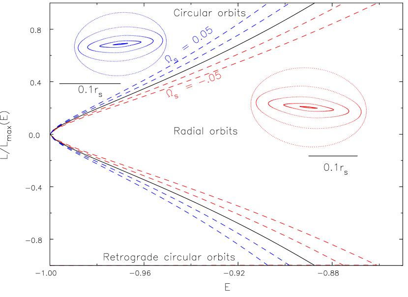
Figure 7.— The solid curve shows the locus of the ILR in the space of energy and fraction of the maximum angular momentum for $\Omega_{b}=0.5$ near the center of a Hernquist halo. The resonance extends to retrograde orbits in which the signs of $\Omega_{\phi}$ and $l$ are reversed. The dashed curves show the loci of orbits that are not precisely resonant, and precess at the rates $\Omega_{s}=\pm 0.025$ and $\Omega_{s}=\pm 0.05$ relative to the pattern. The closed orbits shown are representative of those that precess at $\Omega_{s}=\pm 0.05$ relative to the disturbance; they have a wide range of sizes, with the more eccentric orbits being smaller. The horizontal lines, which have a length of $0.1r_{s}$, show the linear scale for the orbits.

5.1. Inner Lindblad Resonance

As Weinberg and his collaborators have reported, I find that the inner Lindblad resonance (ILR) is the most important in the early stages of these particular experiments with massive, skinny bars. In Paper I, I found that corotation and the direct radial resonance were the two most important resonances when using more realistic bars in simulations that evolved on a much longer timescale and produced little density change. The relative importance of the different resonances in individual cases depends on the radial variation of the quadrupole field strength and the density of particles as functions of the actions, as described in WK07a.

The solid curve in Figure 7 shows the locus of the ILR in the space of energy and fraction of the maximum angular momentum $L_{\rm max}$ for a quadrupole perturbation with $\Omega_{b}=0.5$ in the Hernquist halo. The range of $E$ shown is strongly restricted to the part deep in the center of the potential. The condition for the resonance is $\Omega_{b}=\Omega_{\phi}-\Omega_{r}/2$, where $\Omega_{r}$ and $\Omega_{\phi}$ are respectively the uniform angular frequencies of the radial and azimuthal motion of the particles (Binney & Tremaine 1987, hereafter BT87, ch2). The solid curve in the figure shows that more eccentric resonant orbits are more tightly bound (have lower $E$) than more nearly circular orbits. The lower half of this Figure shows the similar resonance for retrograde orbits for which $\Omega_{b}=\Omega_{\phi}+\Omega_{r}/2$, with $\Omega_{\phi}$ negative.

As described in BT87 (ch 6) orbits at the ILR drawn in a frame that rotates with the perturbation are stationary ellipses. Lynden-Bell (1979) pointed out that one can regard nearly resonant orbits as pursuing ellipses that precess relative to the pattern at the slow angular rate $\Omega_{s}=\Omega_{b}-(\Omega_{\phi}-\Omega_{r}/2)$. The dashed curves in Fig. 7 show the loci of lines of constant $\Omega_{s}$ along which all orbits precess at the same slow rate relative to the pattern.

The sign of the average angular momentum exchange between nearly resonant orbits and the perturbation is determined by their relative precession rate. Orbits with small positive $\Omega_{s}$ gain $L$ on average, while those with negative $\Omega_{s}$ lose on average; the net effect at the resonance depends on the relative numbers of gainers and losers, which depends on the gradient of the particle density in frequency across that resonance.

5.2. Coverage

In order to show that the simulations are capturing the resonant behavior properly, Holley-Bockelmann et al. (2005) and WK07b determine the difference between the density of particles at two different times in the space of the two integrals $E$ and $L$ (more precisely $L/L_{\rm max}(E)$). They evaluate the density in this space from the particles in the simulation using a smoothing kernel, and color code regions by the change in density between the two times. They also draw the loci of several resonances and call attention to the changes associated with resonances.

Their diagnostic therefore requires phase space to be so densely populated that the appropriate change in density occurs at every point in the 2-D space of these integrals, which requires many particles at each point and a very large number in total. However, the resonance extends over a long path through this space, and it is unnecessarily stringent to insist that the correct balance between gainers and losers be fulfilled separately at each point. Instead, the balance need be realized for all resonant particles, which requires many times fewer particles.

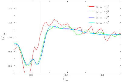
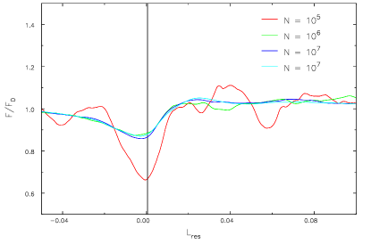
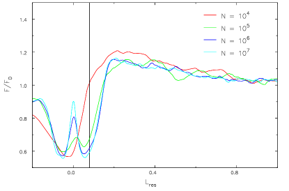
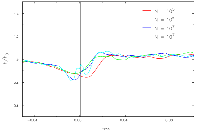
Figure 8.— The ratio $F(L_{\rm res})(t)/F(L_{\rm res})(0)$ for the ILR for two convergence sequences shown in Fig. 4. The left panels are for $t=8$ for the long bar ($a=r_{s}$) while the right panels are for $t=4$ in the cases with $a=r_{s}/5$. The top panels employ a fixed kernel width for all cases, while the kernel width is reduced as $N$ rises in the bottom panels. The vertical lines mark the instantaneous position of the ILR in each case, which is $L_{\rm res}\sim 5\times 10^{-4}$ for the rapidly rotating short bar. The cyan line for the short bar case is for unequal mass particles, particles have equal mass in all other cases.

5.3. A Superior Diagnostic

To demonstrate that the appropriate resonant exchanges are occurring at much lower particle numbers than WK07a suggest are needed, I compute the average density change along lines of constant frequency difference $\Omega_{s}$, such as the dashed lines in Fig. 7. The average so defined is a function of the single variable $\Omega_{s}$, but since this is not an intuitive quantity, I map $\Omega_{s}$ to the quantity $L_{\rm res}$, the angular momentum of the circular orbit that precesses at the rate $\Omega_{s}$ relative to the perturbation.

In practice, I compute the frequencies $\Omega_{r}$ and $\Omega_{\phi}$ for every particle in the simulation in the spherically averaged potential at some moment during the evolution. I compute the frequency difference $\Omega_{s}$ for a selected resonance and evaluate the density of particles at each $\Omega_{s}$ using a 1-D kernel estimate. Then the relation between $\Omega_{s}$ and $L_{\rm res}$ yields the 1-D function $F(L_{\rm res})$ at the selected time (Paper I). This diagnostic is therefore both easier to show and less affected by shot noise than is the density of particles as a function of the two classical integrals $E$ and $L$.

Once the halo density profile starts to change in these experiments, the spherically averaged gravitational potential and the resonant locus also change. I therefore focus here on the early stages before this complication becomes important, although $F(L_{\rm res})$ can be computed with a little more effort for any arbitrary potential, as shown in Sellwood & Debattista (2006).

Figure 8 shows the ratio of $F(L_{\rm res})$ to its initial value for the ILR in the convergence tests shown in the top and middle rows of Fig. 4. The quantity shown is the ratio of $F(L_{\rm res})$ to its undisturbed value for different values of $N$. The left panels show results at $t=8$ for the long bar ($a=r_{s}$) and the right panels at $t=4$ for the short bar ($a=r_{s}/5$). The upper panels show the results with a fixed kernel width, while the width of the smoothing kernel is halved for every factor 10 increase in $N$ in the lower panels. The cyan curve in the right panels is for unequal mass particles with a further reduction of the smoothing kernel width in the lower panel.

As $N$ is increased by three orders of magnitude in the large bar case (left panels), the results quickly converge when a fixed kernel is employed (upper). Reducing the kernel width as $N$ rises (lower) reveals more detail of the function shape. Even for the smallest particle number ($N=10^{4}$), the function shows a substantial change associated with the resonance, but lacks the central spike at $L_{\rm res}=0$ visible in the other cases. The local maximum at $L_{\rm res}=0$ arises because particles of very low angular momentum have orbits that precess at such a high rate they are well inside the ILR and their angular momenta are little affected by the perturbation. The kernel width is too large to reveal this feature in the $N=10^{4}$ case.

Results for the short bar are shown on the right, which again quickly converge with a fixed kernel width (upper). When the kernel width is decreased (lower), a central spike appears only in the case of unequal mass particles (cyan line), for which I also refined the radial grid to place more shells in the inner parts. Note that the resonance is still well-populated in the other three experiments, since $F(L_{\rm res})$ is strongly affected in the appropriate sense, and the time evolution of the pattern speed and density profile, shown by the dotted curves in the middle row of Fig. 4, are no different from those in the coarser experiments. The number of equal mass particles above the resonance in these cases is too small to reveal the spike, whereas the unequal mass case packs in many high frequency particles; clearly, adding particles that are adiabatically invariant to the perturbation can have no effect on the outcome.

6. Discussion

6.1. Frequency broadening

The range of $L_{\rm res}$ over which the ratio departs from unity in Fig. 8 indicates the extent of the resonance during this short time interval, and one can count the numbers of particles within this range. For the large bar, in the left panels of Fig. 8, I find fully 10% of equal-mass particles have $\Omega_{s}$ within the range affected by the resonance, but this factor drops to $\gtrsim 0.7\%$ for the shorter bar ($a=r_{s}/5$). While this smaller fraction clearly implies that a larger number of particles is needed in this more delicate case, as already found empirically in Fig. 4, the $\sim 7,000$ resonant particles in a simulation with $N=10^{6}$ are enough to capture the appropriate response. The resonant fraction with unequal particle masses rises to 20%, even in this short bar case, but the evolution is no different.

The fraction of particles that participate in the ILR is far higher than expected in the calculations by WK07a. This is because their estimate of the resonance width neglects frequency broadening due to the time evolution of the perturbation. Resonances are broadened both by the time evolution of the amplitude, which rises smoothly from zero to its full value in 10 time units, and also because the bar slows over an even shorter time interval (see Fig. 4). The initial bar period of the large bar is $\sim 12.5$ time units, which is longer than both the turn-on time and the slow-down time. The bar period for the shorter bars is $\sim 3$ time units initially, and therefore frequency broadening of resonances is slightly less than for the large bars, but is still highly significant.

Thus the estimates from WK07a of the particle numbers required to “cover” the resonance are for very slowly evolving perturbations, and not for realistic experiments that might produce a large density change. It is perplexing that these authors explicitly discount frequency broadening, since Weinberg (2004) has already shown that the pattern speed evolution depends upon the time history of the perturbation – a clear indication that the resonant interactions responsible for friction do depend upon the broadening of the resonance by the time evolution of the perturbation.

6.2. Particle noise

As for the coverage issue, the timescale for bar pattern speed evolution is so rapid in cases in which the halo density is changed that the time-scale for interactions with the bar is very short. Questions of orbit quality in a noisy potential seem of marginal relevance when the location of the resonance moves faster than any reasonable orbit diffusion rate.

From a crude analysis, BT87 find the relaxation time of a collection of $N$ point masses is

$$\tau_{\rm relax}\simeq{0.1N\over\ln N}\tau_{\rm orb},$$ (4)

where $\tau_{\rm orb}$ is a typical orbit period. This is an underestimate of the relaxation time for most collisionless $N$-body methods, which smooth the gravitational field through particle softening, limited mesh resolution, or some form of filtering of the high-spatial frequencies of the potential. To be conservative, I ignore this favorable caveat for now, and continue the argument with the above crude estimate of the relaxation rate.

Since the relaxation time is approximately the time to cause an order unity change to the initial energy of a typical particle, the fractional energy change per orbit $\Delta E/E\sim 10\ln N/N$. If fractional changes in the important frequencies of an orbit scale as the fractional change in energy of the orbit (this appears to be approximately true in many potentials), orbit scattering will be too slow to affect resonant interactions as long as the fractional change in the bar frequency in one orbit

$$\left|{\Delta\Omega_{b}\over\Omega_{b}}\right|\gg{10\ln N\over N}.$$ (5)

This very crude estimate suggests that relaxation is utterly irrelevant when $|\Delta\Omega_{b}/\Omega_{b}|\sim 1$ in one orbit (e.g., Fig. 4), and will not become an issue except for very mildly braked bars simulated with small numbers of particles. Again WK07a conclude that much larger numbers of particles are needed because their analysis fails to take the changing pattern speed of the perturbation into account.

6.3. Self-gravity methods

Relaxation is conventionally thought of as the cumulative effect of pair-wise encounters between particles, as above, but it can also be regarded as the effect of square root of $N$ type excitations of a number of neutral modes of the equilibrium system, as remarked by Sellwood (1987) and calculated by Weinberg (2001). WK07a attempt to separate $N$-body fluctuations into small- and large-scale noise and appear to associate simple 2-body scattering with small-scale noise and large-scale noise with that from the neutral modes excited by shot noise in the particle distribution (Weinberg 2001). Such a distinction is artificial, since both approaches describe the same physical process.

Hernquist & Barnes (1990) and Hernquist & Ostriker (1992) measured very similar relaxation rates in spherical models simulated by various $N$-body methods. Their important finding can be understood from either approach. First, the Coulomb logarithm appears in the expression for the relaxation rate because every decade of impact parameters contributes equally (BT87). As collisionless $N$-body methods have a limited range of spatial resolution, the number of decades over which scattering must be integrated is strictly limited, and not very different from method to method. Second, only a limited number of neutral modes affect the behavior of an $N$-body simulation, because softening, grid resolution, or truncation of the field expansion quickly cuts off the dynamical influence of the higher modes that have shorter wavelength. Thus either conceptual approach to the influence of noise leads to the same conclusion that no valid $N$-body method is dramatically less collisional than any other (Hernquist & Barnes 1990). (Methods that do not employ many particles per effective softening volume should manifest higher relaxation rates.)

WK07a argue correctly that a well-chosen basis allows forces from unwanted fluctuations on small spatial scales to be filtered out. Despite this, Hernquist & Ostriker (1992) found little improvement in the relaxation rate from this method over others. Thus we conclude that all methods filter out all but the longest range encounters, unless resolution is taken to extreme, leading to at most marginal differences of quality between different methods.

6.4. Previous work

The ability of $N$-body simulations to capture resonant exchanges with a perturbation has previously been demonstrated in the case of disk instabilities. Global modes that lead to bars rely on the emission of angular momentum at the ILR and its absorption at other resonances farther out in the disk (e.g., Kalnajs 1977). Since the mode is driven by 2nd-order coupling between the particles and the wave at resonances, the dynamics resembles that of bar-halo coupling in 3-D. In particular, the third action for each orbit is zero for precisely spherical potentials, making the unperturbed motion of each halo particle no more complicated than in 2-D. It is worth noting that Rybicki (1972) pointed out that 2-D disks are essentially more collisional than 3-D systems, which would argue that if relaxation were an important problem, it ought to be harder to get disks right.

Sellwood (1983), Sellwood & Athanassoula (1986) and Earn & Sellwood (1995) report they are able to reproduce the global bar modes of some disks in simulations with comparatively modest numbers of particles. Tests of a disk without velocity dispersion, employing a large softening length to inhibit local instabilities, may not be a fair comparison with 3-D systems. However, Earn & Sellwood (1995) present results for disks with velocity dispersion using both a field method and a 2-D polar grid. The predicted eigenfrequency was reproduced to within 5% percent using a field method with as few as 15K particles, and agreement with theory improved for moderately larger $N$. Results with the polar grid were discrepant because gravity softening was required, but Fig. 4 of that paper shows that the trend with softening length could plausibly extrapolate back to the predicted frequency at zero softening.

These reassuring results indicate that simulations do indeed capture the appropriate collective response at resonances, without requiring vast numbers of particles. Again the dynamical response of the collection of particles extends over the entire resonance, broadened by the growth-rate of the bar, and does not need to reproduce the detailed balance of gainers and losers at every point in integral space.

6.5. Numerical convergence

WK07a argue that numerical convergence alone is not a guarantee that the result is correct. They suggest that low-$N$ experiments could converge to the wrong result, where friction is determined by one-time encounters between the particles and the bar, while the proper resonant behavior would not be revealed until some much larger particle number is reached.

This argument is unconvincing for several reasons. First, if coverage were inadequate, as WK07a note, the exchange of angular momentum with the bar would depend on just the few particles that happened to be in resonance, resulting in significant stochasticity in the evolution. The pattern speed and density changes would depend on the random seed, which I do not observe, and the curves in Fig. 4 could not overlay so perfectly. Second, as shown in Fig. 8, I have been able to detect the influence of resonances over a wide range of $N$. Third, WK07b estimate that $N\gtrsim 10^{8}$ equal mass particles should be sufficient for a strong bar with semi-major axis equal to the profile break radius $r_{s}$. I have presented a result with $N=1.6\times 10^{8}$ that behaves no differently from experiments with much lower $N$. This sequence of experiments therefore demonstrates that nothing different occurs when their criteria are met.

WK07b present a result for a strong bar with length equal to $r_{s}/6$ in which the evolution differs when $N$ is increased from $10^{6}$ to $5\times 10^{6}$. I have been unable to reproduce a change in behavior at any $N$ in tests with similar, though not identical, bars; their bar had an axis ratio of 5:1, which I have also used, but since it is possible the quadrupole field of their bar is weaker than given by eq. (3), I chose to present a 4:1 bar in the bottom row of Fig. 4 (as described in §4.1). It is unclear why WK07b find a different result with different $N$, but my failure to observe differences of this kind in a similar regime suggests that the difference they report must be due to factors other than they suggest.

7. Halo density reduction

7.1. Cusp flattening

Figure 9 compares the mass evolution in the fiducial run, for unequal mass particles, with that when the monopole term of the halo mass distribution is held fixed. It should be noted that these two runs differ only in the monopole terms, the gravitational field from the $2\leq l\leq 4$ density response of the particles is included in both cases. It is clear that including the change in the potential that arises from the change to the radial mass profile is crucial for creating a large density reduction, as previously found for driven bars (Sellwood 2003).

Figure 9.— The changes to the mass profile for the fiducial bar with the monopole term active (solid curves) and in an identical case when the $l=0$ term of the halo mass distribution is held fixed (dashed). These experiments employed $10^{7}$ unequal mass particles.

Thus flattening of the cusp is a collective effect that is suppressed when the self-consistent potential changes are eliminated. Once the collective change is initiated, the different radial mass profile allows somewhat more angular momentum to be accepted by the resonant particles; the torque in the self-consistent case is some 20% larger at its peak, near $t=8$, than when the central attraction is held fixed. This is physically reasonable, since adjustments to the central attraction of the mass distribution will further broaden the resonances. Note that the self-consistent density change could not be predicted from simple perturbation theory, since the global potential in which the particles move undergoes substantial evolution on an orbital time-scale during the cusp-flattening stage (see Fig. 3).

WK07b report much smaller density reductions than I find with similar strong, skinny bars. It is likely that the collective effect I find to be responsible for large density reductions is inhibited by the rigid mass component they include. To test this hypothesis, I have tried similar experiments that include the rigid bar monopole term and find that density reduction is almost entirely suppressed.

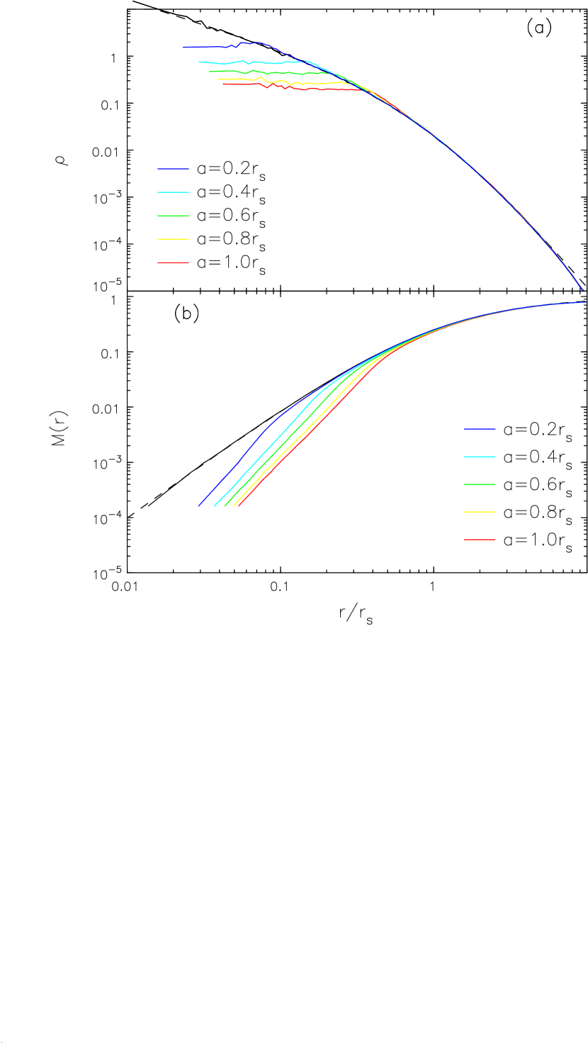
Figure 10.— Results from five different experiments with different bar lengths. (a) The dashed line shows the initial profile given by eq. 2. The solid lines show estimates from the particles of the initial (black) and final (color) density profiles from a series of runs with different bar semi-major axes, $a$. (b) The same results plotted as halo mass enclosed as a function of radius.

7.2. Variation of bar properties

Here I report the results of changing the physical parameters of the bar perturbation: its length, mass, and axis ratio.

Figure 10 shows the final density profiles from a series of five separate simulations using bars of different lengths. The lengths span the range $0.2\leq a\leq 1$, in equal steps of $\Delta a=0.2$, while the nominal bar axis ratios are kept at $a/b=5$ and $a/c=10$. As above, the bar mass is half the enclosed halo mass at $r=a$ and the initial pattern speed places corotation at the bar end. In all experiments shown in Fig. 10, the final halo density is flattened inside $r\simeq 0.3a$, while remaining essentially unchanged at larger radii.

Figure 11.— Solid lines show the initial and final mass profiles from a series of runs in which the bar axis ratio $b/a$ was varied. The pronounced gap in the final mass profiles is bracketed by two runs in which $b/a=0.32$ and $b/a=0.30$; the dotted lines show reruns of these models with more individual-mass particles. The dashed line shows the Hernquist profile.

Figure 12.— As for Fig. 11, but from a series of runs in which the bar mass was varied. The sharp transition occurs between $0.0625\leq M_{b}\leq 0.07$.

Figure 13.— Results near the sharp transition. (a) Circles indicate the cusp flattened for the bar mass and axis ratio, while squares indicate it did not. The bar semi-major axis is held constant at $a=r_{s}$ in all cases. (b) The quadrupole potential along the bar major axis given by eq. (3) for the bars in the simulations shown in (a). Bar potentials that caused the cusp to flatten are drawn with solid lines, those that did not are dashed.

Figure 11 shows the effect of changing the bar axis ratio $b/a$. The nominal bar axis ratios in the models shown range from $a/b=5$ to $a/b=2$; in all cases, $a=r_{s}$, $M_{b}=0.125$, and $\Omega_{b}=0.5$ initially. The more elliptical bars produce large density changes, whereas rounder bars have little effect. A sharp transition is evident in these results between $0.30<b/a<0.32$. Tests with the SCF method (Hernquist & Ostriker 1992) also reveal the sharp transition at the same bar axis ratio.

A similar effect is seen in Figure 12, in which $0.050\leq M_{b}\leq 0.125$, i.e. the bar mass ranges from 20% to 50% of the enclosed halo mass, while the bar axis ratio is held fixed at $b/a=0.2$. The sharp transition occurs between $0.0625\leq M_{b}\leq 0.07$.

7.3. Sharp transition

The bimodal nature of the density change shown in Figs. 11 & 12 appears to be real. The models evolve more slowly as friction is weakened by reducing the bar quadrupole field, either by making the bar rounder or by reducing its mass, but the halo density change undergoes an abrupt transition as the parameter is varied smoothly.

Figure 14.— Above: The angular momenta of the bar (decreasing dashed) and of the halo (increasing dashed) and total (solid) in two simulations straddling the boundary between cusp flattening and more gradual density change. That on the left had $b/a=0.30$ while that shown on the right had $b/a=0.32$. Below: The radii containing different fractions of the total number of particles in the two cases.

Figure 13(a) shows results in the space of the two parameters $a/b$ and $M_{b}$ from experiments run to map out the transition boundary, always for the case of the long bar with $a=r_{s}$. The quadrupole fields of the bars are shown in Fig. 13(b). This Figure suggests that there is a critical quadrupole field strength required to cause the cusp to flatten, which may decrease slightly towards skinnier bars where the quadrupole peaks at smaller radii.

It is unclear what triggers the collective response. Figure 14 shows more information from the two cases that straddle the sharp transition in the density change as the axis ratio is changed. The angular momentum absorbed by the halo (upper panels) differs very little between the two cases, yet the slightly stronger bar flattened the cusp at late times (after most of the angular momentum had been lost) while the other did not. I have checked that no dramatic density changes occur in the cases with weaker quadrupoles, no matter for how long the simulations are continued. Friction tails off at late times in these runs without producing a large density change.

Notice also the clear time sequence in the density reduction (lower left panel); the density in the outer part of the cusp is reduced before that in the inner part.

The mass profile evolution is insensitive to numerical parameters everywhere except near the transition. §4 presented numerous tests to show that the evolution of these simulations does not depend on numerical parameters. Since WK07b argue that more delicate cases require larger $N$, I simulated the large, massive bar model with $b/a=0.32$ with $1.6\times 10^{8}$ unequal mass particles, finding a small change to the mass profile that is no different from that in simulations with lower $N$.

However, the outcome of experiments for the marginal case of the large, massive bar with axis ratio $b/a=0.31$ does depend on numerical parameters. In some cases the cusp flattens while in others it does not; the result is never intermediate, however. Thus these simulations cannot pin down the parameter values at which the outcome changes to better than a few percent.

I have searched the experimental results for a property that could be the cause of the sharp transition. I examined resonant exchanges in two simulations that straddle the boundary using the procedure described in §5, finding only very minor differences in $F(L_{\rm res})$ between the two cases. The ILR continues to be the most important resonance, even at late times when the pattern speed is about 20% of its initial value; friction is weak and changes to $F(L_{\rm res})$ are correspondingly small, but still detectable. Other properties, such as the amplitude of the bisymmetric distortion in the halo response, all varied smoothly with the strength of the quadrupole field.

While the trigger for the collective response that brings about the large density change remains elusive, further investigation seems warranted only if a similar sharp transition were found in fully self-consistent models.

Table 2Summary of simulations plotted in Figure 15

$M_{b}$	$a$	$b$	$\delta\lambda$	$\mu$	fltnd	MoI
0.0139	0.2	0.04	0.00006	0.59595	y
0.0408	0.4	0.08	0.00033	0.25639	y
0.0703	0.6	0.12	0.00096	0.15082	y
0.0988	0.8	0.16	0.00184	0.09279	y
0.125	1.0	0.20	0.00288	0.06936	y
0.0139	0.2	0.04	0.00024	0.44957	y	5
0.125	1.0	0.20	0.00288	0.06936	y
0.1	1.0	0.20	0.00236	0.08386	y
0.075	1.0	0.20	0.00176	0.11818	y
0.07	1.0	0.20	0.00176	0.12763	y
0.0625	1.0	0.20	0.00156	0.60344	n
0.050	1.0	0.20	0.00113	0.84208	n
0.050	1.0	0.20	0.00514	0.74350	n	5
0.125	1.0	0.20	0.01215	0.04334	y	5
0.0625	1.0	0.20	0.00629	0.10646	y	5
0.125	1.0	0.25	0.00283	0.07789	y
0.125	1.0	0.27	0.00298	0.08104	y
0.125	1.0	0.29	0.00315	0.09306	y
0.125	1.0	0.30	0.00323	0.09352	y
0.125	1.0	0.31	0.00312	0.34321	y
0.125	1.0	0.33	0.00274	0.70371	n
0.125	1.0	0.50	0.00296	0.91227	n
0.125	1.0	0.33	0.00982	0.04764	y	5
0.125	1.0	0.50	0.00874	0.89144	n	5
0.125	1.0	0.50	0.01378	0.83108	n	10

7.4. More gradual density changes

The large density changes emphasized so far are confined to the region well interior to the end of the bar. They result from a collective response of the halo particles to the torque from a massive, skinny bar. The perturbing potential is not only stronger than that of the nominal homogeneous ellipsoidal bar (see Appendix), but is also not easily related to bars in real galaxies that may have somewhat different quadrupole fields. However, it seems unlikely that real bars, which typically have $a/b\lesssim 3$, are strong enough to provoke such a collective halo response.

The bars that did not produce large density changes are still strong, both in mass and in axis ratio. Friction from these bars does lead to a slight reduction in halo density over a more extended radial range; tests reported in Paper I and further tests here confirm that these results are also insensitive to numerical parameters. It is likely that the modest mass profile change reported by Debattista & Sellwood (2000), and those discernible in Athanassoula’s (2003) results are of this kind.

Figure 15.— Fractional changes, $\mu$, to $\Delta_{v/2}$ in many experiments. The abscissae show the angular momentum given to the halo, expressed as the usual dimensionless spin parameter. Open circles mark results from experiments in which the density profile of the inner cusp was flattened, while squares indicate experiments where cusp flattening did not occur. Filled symbols show results from experiments in which the MoI of the bar was increased by a factor 5 in all cases except the point at the upper right, where the MoI was increased 10-fold. The changes to $\Delta_{v/2}$ make no allowance for halo compression. The bar parameters in each case are listed in Table 2.

8. Mean Density Reduction

8.1. Changes to $\Delta_{v/2}$

This study was motivated by the discrepancy, illustrated in Fig. 1, between the predictions of halo density from LCDM and that observed in real galaxies. The solid and dashed lines in that Figure show the predicted value of $\Delta_{v/2}$ (Alam et al. 2002) for dark matter halos, that are generally above the observed points. If bar-halo friction could effect a reduction of the mean inner halo density by about one order of magnitude, as measured by $\Delta_{v/2}$, the predicted lines could be shifted down by that factor and the discrepancy between the predictions and the data would be largely removed.

Since the halo parameters of mass and linear size in my simulations can be scaled as desired, the only quantity of relevance that can be extracted from them is the fractional change in $\Delta_{v/2}$: $\mu=\hbox{$\Delta_{v/2}$}(t)/\hbox{$\Delta_{v/2}$}(0)$. Figure 15 shows the fractional change to the inner halo density, $\mu$, measured from the simulations listed in Table 2. Results presented are exclusively from cases that are numerically converged – i.e. results from low-$N$ simulations in convergence tests are excluded. Circles mark results from experiments in which the density profile of the inner cusp was flattened. Weaker bars of any length lead to mild density reductions, as shown by the points marked with squares. The largest reductions to $\Delta_{v/2}$, by a factor $\mu^{-1}\gtrsim 10$, occur when the inner part of the cusp is flattened by exchanges with a long ($a=r_{s}$) bar. Strong short bars also flatten the cusp, but over a smaller volume, leading to a smaller reduction in $\Delta_{v/2}$.

The density reductions possible with rigid bars may underestimate the largest that can be achieved, since real stellar bars are not rigid objects with pattern speeds that decrease as dictated by a fixed moment of inertia (MoI) as angular momentum is removed. The stars within the bar must lose angular momentum, but the pattern speed of the bar is determined by the mean precession rate of the orbits. (It could even rise as the orbits shrink in size, although such behavior has not been reported in any simulation, as far as I am aware.) Thus adopting the fixed MoI of a homogeneous ellipsoid may seriously underestimate the angular momentum that could be extracted from the bar.

Accordingly, I experimented with bars in which the effective MoI was increased by a factor of five or ten from the standard value employed so far, as noted in Table 2. This stratagem resulted in a correspondingly greater transfer of angular momentum to the halo over a more protracted period as the pattern speed declined more slowly, and the results are shown by the filled symbols in Figure 15. The enhanced MoI caused a greater reduction in the inner halo density than in comparable experiments with the standard MoI, but by a significant factor only if cusp flattening occurred.

A decrease in $\Delta_{v/2}$ by a factor $\gtrsim 10$ requires a large ($a=r_{s}$), massive, skinny bar, and the greatest changes occur when the MoI of such bars are increased. The density reduction by a shorter bar, $a=0.2r_{s}$, is to about 60% of the original $\Delta_{v/2}$, which can be boosted to $\sim 45\%$ by increasing the MoI.

8.2. Angular Momentum Extracted from the Bar

It is useful to express the angular momentum transferred to the halo in terms of the usual dimensionless spin parameter, $\lambda=LE^{1/2}/GM^{5/2}$. Tidal torques lead to halos with a log-normal distribution of spin parameters with a mean $\lambda\sim 0.05$. Assuming, as usual, that the baryons and dark matter are well mixed initially, the fraction of angular momentum in the baryons is equal to the baryonic mass fraction: some 10% – 20%.

The abscissae in Fig. 15 show the angular momentum transferred to the halo, expressed as a change to $\lambda$. Thus the angular momentum that must be transferred from the baryons to the dark halo to increase its spin parameter by $\Delta\lambda_{\rm b}\sim 0.01$ requires the removal of all the angular momentum that could reasonably be expected to be possessed by the baryons! This conclusion suggests that no greater density reductions could be achieved by this method. Note that as the estimates of halo density in Fig. 1 are all from rotationally supported disks, these galaxy disks must retain a significant fraction of their initial angular momentum.

Since I have excluded the monopole term of the bar potential, and kept the bar quadrupole fixed, these experiments ignore effects that increase the halo density. The halo must be compressed as baryons cool and settle to make the disk, and contraction of a self-consistent bar as it loses angular momentum can cause the halo to compress further (Sellwood 2003; Colín et al. 2006), overwhelming any density reduction caused by the angular momentum transferred. Thus the changes to $\Delta_{v/2}$ reported in Fig. 15 are likely to be overestimates.

9. Conclusions

I have shown that reliable results can be obtained from careful simulations of self-gravitating halos perturbed by a rigid bar without the need for immense numbers of particles. Rigid bars are an idealization, but simplify the dynamics down to the bare essentials over which disagreements remain.

Weinberg & Katz (2007a) estimate the required numbers of particles from perturbation theory. Their “coverage” criterion is based on a requirement that there be enough particles in a narrow range of frequencies around the resonance to yield the correct statistical balance between gainers and losers in resonant interactions. Their criterion, however, takes no account of the time-dependence of the perturbation, which causes resonances to be broadened over a wide range of frequencies allowing the correct response to be captured with a much smaller $N$. The excessive requirements suggested by WK07a apply to the numerically much more delicate case of a steadily rotating, fixed amplitude perturbation. Furthermore, their diagnostic diagrams require detailed balance at each point in $(E,L)$-space, whereas the balance must be right for the complete ensemble of resonant particles, which is a much larger fraction of the total. My Fig. 8 shows that simulations do indeed manifest resonant exchanges with the perturbation that include a significant fraction of the particles and the resonant response converges at moderate $N$. Larger particle numbers enable the changes at resonances to be illustrated in more detail, but the physical outcome of the experiments is no different.

The minimum number of particles needed to obtain a converged result does depend slightly upon the bar properties, and can be lowered by adopting unequal mass particles. I have shown that neither the angular momentum transferred nor the halo density change varies as $N$ is increased above $\sim 10^{5}$ equal mass particles for long, massive, skinny bars. Simulations with over $10^{8}$ particles, which meet the criteria suggested by WK07a, do not behave any differently from those with three orders of magnitude fewer particles. Shorter bars do require more care than do large bars, but again I find the behavior converges at moderate $N$, and that $10^{8}$ unequal mass particles is far more than is needed.

Above this modest minimum number of particles, I find that results from a grid code are identical to those obtained using the field method devised by Hernquist & Ostriker (1992), as explained in §6.3. Results with different $N$, or with different random seeds, show none of the stochasticity expected if there were too few particles in any of the dynamically important resonances.

Mild bars, for which evolution is slower, require greater care; e.g., my convergence test for the pattern speed evolution with self-gravity (Fig. 13 of Paper I) indicated that $N\gtrsim 10^{6}$ was required for a very mild bar ($a=r_{s}$, $a:b=1:0.5$, and $M_{b}=0.02$ or 8% of the enclosed halo mass). However, such more delicate cases are incapable of effecting a substantial density reduction (§8).

WK07a also invoke orbit scattering by density fluctuations as a second reason to require large $N$. In simulations where the halo density reduction is substantial, the bar is slowed on an orbit timescale, which is always much shorter than the relaxation timescale (Binney & Tremaine 1987), leading to a much lower particle number requirements (§6.2). Furthermore, the experimentally determined mass profiles are very smooth, and the radial acceleration will have correspondingly little noise. While this argument ignores fluctuations in non-axisymmetric forces, I find my results are also insensitive to changes in the order of azimuthal expansion (Fig. 5).

These results indicate that the estimates of the required numbers of particles given by Weinberg & Katz are greatly exaggerated. The evidence I have presented continues to indicate that careful simulations with ${\cal O}(10^{6})$ halo particles yield reliable indications of the evolution of both the pattern speed and density profile.

I have also determined the amount of halo density reduction that can be brought about through angular momentum transfer from a strong, initially rapidly-rotating bar, again with the limitation that the simulations are not fully self-consistent. My simulations with massive, skinny bars confirm earlier work that the densities of cusped DM halos can be reduced by bar-halo interactions. However, I also show that more moderate bars are able to achieve no more than a minor reduction in the mean density of the inner halo, when halo compression is neglected.

I have found that large density reductions occur only when the inner cusp is flattened to create a uniform density core, which I show extends to a radius of about 1/3 the bar semi-major axis. I have demonstrated that flattening of the inner cusp is a collective response of the halo that is driven by the bar torque.

In sequences of experiments in which the mass or axis ratio of the rigid bar is gradually weakened, I find an abrupt change of behavior from cusp flattening, to mild density reductions. The sharp transition as the bar quadrupole field is weakened appears to be real. Behavior on either side of the sharp transition is independent of the numerical parameters or the code used. Pairs of simulations straddling the boundary behave bimodally and results are never intermediate. Since I have found that triggering of the collective effect in truly marginal cases does depend on numerical parameters, the parameter values at which the outcome changes cannot be determined precisely from simulations. However, I emphasize again that the outcome of all simulations reported in this paper is independent of all numerical parameters, aside from an extremely narrow range around this boundary.

A reduction of the mean inner density by an order of magnitude requires a bar, having a semi-major axis equal to the break radius of the halo density profile, i.e. $\sim 12-20\;$kpc, axis ratio $a/b\gtrsim 3$, and bar mass $\gtrsim 30\%$ of the enclosed halo mass. Large reductions must be offset in part, and mild reductions overwhelmed, by halo compression through baryonic settling, which has not been included here.

Real bars probably have higher effective moments of inertia allowing more angular momentum to be extracted from them. Experiments to mimic this effect resulted in somewhat larger density reductions for a given bar; for reasonable bars, the overall density reduction remained less than a factor two. Extreme bars with enhanced moments of inertia also achieved greater density reductions, but at the cost of transfering more angular momentum to the halo than the baryons are likely to possess.

The angular momentum available in the baryons limits the density reduction achievable by bars. Since the galaxies for which halo density measurements are available in Fig. 1 are all still rotationally supported, the baryons cannot have invested all their angular momentum into halo density reduction. External perturbers, such as massive companions, undoubtedly contain more angular momentum and energy in orbital motion, and therefore may seem to have the potential to achieve greater reductions. It should be noted, however, that merging is a process already taken into account in the predicted profiles, since individual halos generally result from a series of mergers (e.g. Wechsler et al. 2002).

The density reductions reported here are overestimates of those possible in reality, since I did not include the monopole terms of the bar field. A massive disk, in which the bar forms, must have compressed the halo as the baryons settle towards its center, and the mean density of the inner halo will have risen by perhaps a factor of three (e.g. Sellwood & McGaugh 2005). Furthermore, loss of angular momentum from the bar causes it to contract further, producing yet more halo compression that may even overwhelm any reduction in halo density resulting from the angular momentum transfer (Sellwood 2003; Colín et al. 2006).

REFERENCES

Alam, S. M. K., Bullock, J. S. & Weinberg, D. H. 2002, ApJ, 572, 34

Athanassoula, E. 2002, ApJ, 569, L83

Athanassoula, E. 2003, MNRAS, 341, 1179

Binney, J. & Evans, N. W. 2001, MNRAS, 327, L27

Binney, J., Gerhard, O. & Silk, J. 2001, MNRAS, 321, 471

Binney, J. & Tremaine, S. 1987, Galactic Dynamics (Princeton: Princeton University Press) (BT87)

Bullock, J. S., Kolatt, T. S., Sigad, Y., Somerville, R. S., Kravtsov, A. V., Klypin, A. A., Primack, J. R. & Dekel, A. 2001, MNRAS, 321, 559

Ceverino, D. & Klypin, A. 2007, MNRAS, 379, 1666

Chandrasekhar, S. 1969, Ellipsoidal Figures Equilibrium (Dover)

Colín, P., Valenzuela, O. & Klypin, A. 2006, ApJ, 644, 687

Debattista, V. P. & Sellwood, J. A. 2000, ApJ, 543, 704

Diemand, J., Moore, B., Stadel, J. 2004, MNRAS, 353, 624

Earn, D. J. D. & Sellwood, J. A. 1995, ApJ, 451, 533

El-Zant, A., Shlosman, I. & Hoffman, Y. 2001, ApJ, 560, 636

Ferrarese, L. & Merritt, D. 2000, ApJ, 539, L9

Gebhardt, K., et al.  2000, ApJ, 539, L13

Gnedin, O. Y. & Zhao, H.S., 2002, MNRAS, 333, 299

Hernquist, L. 1990, ApJ, 356, 359

Hernquist, L. & Barnes, J. E. 1990, ApJ, 349, 562

Hernquist, L. & Ostriker, J. P. 1992, ApJ, 386, 375

Hernquist, L. & Weinberg, M. D. 1992, ApJ, 400, 80

Holley-Bockelmann, K., Weinberg, M. & Katz, N. 2005, MNRAS, 363, 991

Jardel, J. & Sellwood, J. A. 2008, ApJ, submitted

Kalnajs, A. J. 1977, ApJ, 212, 637

Klypin, A., Zhao, HS. & Somerville, R. S. 2002, ApJ, 573, 597

Kuzio de Naray, R., McGaugh, S. S., de Blok, W. J. D. & Bosma, A. 2006, ApJS, 165, 461

Lynden-Bell, D. 1979, MNRAS, 187, 101

Marinova, I. & Jogee, S. 2007, ApJ, 659, 1176

McGlynn, T. A. 1984, ApJ, 281, 13

McMillan, P. J. & Dehnen, W. 2005, MNRAS, 363, 1205

Milosavljević, M., Merritt, D., Rest, A. & van den Bosch, F. C. 2002, MNRAS, 331, L51

Navarro, J. F., Eke, V. R. & Frenk, C. S. 1997, MNRAS, 283, L72

Navarro, J. F., Frenk, C. S. & White, S. D. M. 1997, ApJ, 490, 493

Navarro, J. F., Hayashi, E., Power, C., Jenkins, A. R., Frenk, C. S., White, S. D. M., Springel, V., Stadel, J, & Quinn, T. R. 2004, MNRAS, 349, 1039

Neto, A. F., Gao, L., Bett, P., Cole, S., Navarro, J. F., Frenk, C. S., White, S. D. M., Springel, V. & Jenkins, A. 2007, MNRAS, 381, 1450

Power, C., Navarro, J. F., Jenkins, A., Frenk, C. S. & White, S. D. M. 2003, MNRAS, 338, 14

Reese, A., Williams, T. B., Sellwood, J. A., Barnes, E. I. & Powell, B. A. 2007, AJ, 133, 2846

Rhee, G., Valenzuela, O., Klypin, A., Holtzman, J. & Moorthy, B. 2004, ApJ, 617, 1059

Rybicki, G. B. 1972, in IAU Colloq. 10, Gravitational $N$-body Problem, ed. M. Lecar (Dordrecht: Reidel), 22

Sellwood, J. A. 1983, J. Comp. Phys., 50, 337

Sellwood, J. A. 1985, MNRAS, 217, 127

Sellwood, J. A. 1987, ARA&A, 25, 151

Sellwood, J. A. 2003, ApJ, 587, 638

Sellwood, J. A. 2006, ApJ, 581, 567 (Paper I)

Sellwood, J. A. & Athanassoula, E. 1986, MNRAS, 221, 195

Sellwood, J. A. & Debattista, V. P. 2006, ApJ, 639, 868

Sellwood, J. A. & McGaugh, S. S. 2005, ApJ, 634, 70

Simon, J. D., Bolatto, A. D., Leroy, A., Blitz, L. & Gates, E. L. 2005, ApJ, 621, 757

Spergel, D. N. et al. 2007, ApJS, 170, 377

Swaters, R. A., Madore, B. F., van den Bosch, F. C. & Balcells, M. 2003, ApJ, 583, 732

Tegmark, M., et al. 2006, Phys. Rev. D, 74, 123507

Tremaine, S. & Weinberg, M. D. 1984, MNRAS, 209, 729

Valenzuela, O., Rhee, G., Klypin, A., Governato, F., Stinson, G., Quinn, T. & Wadsley, J. 2007, ApJ, 657, 773

Wechsler, R. H., Bullock, J. S., Primack, J. R., Kravtsov, A. V. & Dekel, A. 2002, ApJ, 568, 52

Weinberg, M. D. 1985, MNRAS, 213, 451

Weinberg, M. D. 2001, MNRAS, 328, 321

Weinberg, M. D. 2004, astro-ph/0404169

Weinberg, M. D. & Katz, N. 2002, ApJ, 580, 627

Weinberg, M. D. & Katz, N. 2007a, MNRAS, 375, 425 (WK07a)

Weinberg, M. D. & Katz, N. 2007b, MNRAS, 375, 460 (WK07b)

Weiner, B. J. 2004, in IAU Symp. 220, Dark Matter in Galaxies, ed. S. Ryder, D. J. Pisano, M. Walker, & K. Freeman (Dordrecht: Reidel), 35

Zánmar Sánchez, R., Sellwood, J. A., Weiner, B. J. & Williams, T. B. 2008, ApJ, to appear (arXiv:0710.5286)

Zentner, A. R. & Bullock, J. S. 2002, Phys. Rev. D, 66, 043003 For a homogeneous bar, Weinberg (1985) adopts the approximate quadrupole potential (his eq. 28)

$$\Phi_{\rm b}(r,\theta,\phi)={b_{1}r^{2}\over 1+(r/b_{5})^{5}}Y_{22}(\theta,\phi-\phi_{0})$$ (1)

where $Y_{22}=\sqrt{15/(32\pi)}\sin^{2}\theta e^{2i(\phi-\phi_{0})}$ and $\phi_{0}$ is the phase of the bar. For a bar with axes $a_{1}:a_{2}:a_{3}$ and density $\rho$, he chooses

$$b_{1}=\pi G\rho\sqrt{8\pi\over 15}(A_{1}-A_{2}),$$ (2)

and

$$b_{5}^{5}=a_{1}a_{2}a_{3}{2\over 5}{a_{2}^{2}-a_{1}^{2}\over A_{1}-A_{2}}.$$ (3)

The dimensionless elliptic integrals, $A_{i}$ are defined by Chandrasekhar (1969 Ch. 3, eq. 18):

$$A_{i}=a_{1}a_{2}a_{3}\int_{0}^{\infty}{du\over(a_{i}^{2}+u)\Delta},$$ (4)

with

$$\Delta^{2}=(a_{1}^{2}+u)(a_{2}^{2}+u)(a_{3}^{2}+u).$$ (5)

Note that the expression for $b_{1}$, eq. (2), is twice that given in eq. (46) of Weinberg (1985), in order to obtain the correct variation in $\Phi_{\rm b}$ between the major and minor axes at small $r$.

Figure 16.— The quadrupole part of the gravitational potential along the major axis of a homogeneous bar with $a/b=2$ (above) and $a/b=5$ (below). The solid curve gives the exact potential, the dashed curve the approximation eq. (3). The approximation matches well at small and large distances, but strongly overestimates the peak for skinny bars. Note the difference in scale of the ordinates between the two panels.

I prefer to write eq. (1) in the form (cf. eq. 3)

$$\Phi_{\rm b}(r,\theta,\phi)=-{GM_{b}\over a}{\alpha_{2}r_{*}^{2}\over 1+(r_{*}/\beta_{2})^{5}}\sin^{2}\theta e^{2i(\phi-\phi_{0})},$$ (6)

with $r_{*}=r/a$ and $a_{1}:a_{2}:a_{3}=a:b:c$. Comparing eqs. (3) & (1), we find that $\beta_{2}=b_{5}/a$ and

$$\alpha_{2}={3a^{2}\over 8bc}(A_{1}-A_{2}),$$ (7)

since $M_{b}=4\pi abc\rho/3$. Table 1 gives the values of $\alpha_{2}$ and $\beta_{2}$ for the bar axis ratios used in this paper (n.b. $a/c=10$ in all cases).

For completeness, the quadrupole potential in Cartesian coordinates is:

$$\Phi_{\rm b}(x,y,z)=-{\alpha_{2}GM_{b}\over a^{3}}{(x^{2}-y^{2})\cos 2\phi_{0}+2xy\sin 2\phi_{0}\over 1+(r/\beta_{2}a)^{5}}.$$ (8)

Writing $\eta=r/(\beta_{2}a)$, $\nu=1+\eta^{5}$ and $\xi=[(x^{2}-y^{2})\cos 2\phi_{0}+2xy\sin 2\phi_{0}]/a^{2}$, this simplifies to

$$\Phi_{\rm b}(x,y,z)\simeq-{GM_{b}\alpha_{2}\over a}{\xi\over\nu}.$$ (9)

The acceleration components are

$$a_{x}={GM_{b}\alpha_{2}\over a^{3}}{2\nu(x\cos 2\phi_{0}+y\sin 2\phi_{0})-5\xi ax\eta^{4}/(r\beta_{2})\over\nu^{2}}\\$$ (10)

$$a_{y}={GM_{b}\alpha_{2}\over a^{3}}{2\nu(x\sin 2\phi_{0}-y\cos 2\phi_{0})-5\xi ay\eta^{4}/(r\beta_{2})\over\nu^{2}}\\$$ (11)

$$a_{z}=-{GM_{b}\alpha_{2}\over a^{3}}{5\xi az\eta^{4}\over r\beta_{2}\nu^{2}}.$$ (12)

Figure 16 compares the exact quadrupole potentials of two homogeneous ellipsoids of different axis ratios with the approximation given by eq. (3); $a/c=10$ in both cases. The values of the parameters $\alpha_{2}$ and $\beta_{2}$ are defined to ensure a good match at small and large distances for bars of any axis ratio, which indeed they achieve. While the approximation is pretty good everywhere for the 2:1 bar (top panel), it increasingly overestimates the peak strength of the quadrupole field as the bar ellipticity increases, as shown for a 5:1 bar (bottom panel).

The exact field, which I used in Paper I, can be determined only numerically, and therefore would not be easy for others to reproduce. Throughout this paper, I have continued to use the approximation given by eq. (3), even though it clearly provides a stronger perturbation than the nominal homogeneous bar when $a/b\gg 2$. The results continue to be of interest, however, since some other density distribution could give rise to this stronger quadrupole.

It is unclear what form of the quadrupole WK07b adopted. The text of their paper states that they used the quadrupole approximation of eq. (3), which is the reason I adopted this expression, but their Figure 3 shows the radial dependence for different axis ratios on logarithmic scales. Since the free parameters simply set the amplitude and radius scales of the function, these curves all ought to be self-similar, but they are not. WK07b give no explanation, but the deviations from the simple fitting function are in the correct sense to provide a better fit to the exact field of a homogeneous ellipsoid.

I have made repeated attempts to reproduce results from WK07b, using NFW halos, including a rigid monopole term of the bar, and experimenting with different approximations to the quadrupole, but have not succeeded in reproducing the pattern speed or density evolution they report for any of their simulations with skinny bars; this contrasts with the success I had (Sellwood 2003) in reproducing a result from Hernquist & Weinberg (1992) for a rounder bar. It seems likely that the quadrupole field they used for the 5:1 bar in their fiducial and other experiments has the form shown in their graph, and not the functional form stated in their paper.