Footpoint versus loop-top hard X–ray emission sources
in solar flares

Abstract

Aims. The hard X-ray flux ratio $\Re$ of the footpoint sources to the loop-top source has been used to investigate non-thermal electron trapping and precipitation in solar flares.

Methods. Considering the mission-long Yohkoh Hard X–ray Telescope database, from which we selected 117 flares, we investigated a dependence of the ratio $\Re$ on flare loop parameters like height $h$ and column depth $N$. We used non-thermal electron beams as a diagnostic tool for magnetic convergence.

Results. The ratio $\Re$ decreases with $h$ which we interpret as an effect of converging field geometry. Two branches seen in the $\Re-h$ diagram suggest that in the solar corona two kinds of magnetic loops can exist: a more-converged ones that are more frequent (above 80%) and less-converged loops that are less frequent (below 20%). A lack of correlation between the ratio $\Re$ and $N$ can be due to a more complex configuration of investigated events than seen in soft X–rays.

Conclusions. Obtained values of the magnetic mirror ratio are consistent with previous works and suggest a strongly nonpotential configuration. Further investigation including RHESSI data is needed to verify our results.

1 Introduction

Images taken by the Hard X–ray Telescope (HXT) onboard Yohkoh show different spatial distributions of hard X–ray emission in solar flares. Classifications of hard X–ray emission sources observed in solar flares have been reported (e.g. Kosugi kosugi (1994), Masuda masuda2 (2002), Aschwanden aschwpodr (2004)). However, an unification is possible in which hard X–ray emission sources are divided into two classes: coronal and chromospheric. Members of the first class usually occur within or above the top of the magnetic coronal loop clearly seen in soft X–rays, thus we call them loop-top or above-the-loop-top sources. Members of the second class occur at the entrance of the same magnetic coronal loops into the chromosphere, thus we call them footpoint sources. For the more complicated morphologies, interacting loops or an arcade of loops, such a division still works, however, more hard X–ray sources can be seen at times.

The majority of flares show the presence of hard X–ray emission sources of both classes: loop-top source and footpoint ones. However, their basic properties are different. The footpoint sources are stronger than the loop-top ones during the hard X–ray bursts of the impulsive phase. Footpoint sources grow with higher-energy photons. At the end of the impulsive phase the footpoint sources fade and the loop-top source becomes brighter but its radiation only rarely exceeds 30 keV.

Energy spectra of hard X–ray photons emitted during the impulsive phase of flares have a non-thermal shape. They can be described by a single or a double power-law function. Usually the energy spectra of footpoint sources are flatter than the spectra of the loop-top sources i.e. the index $\gamma$ of the function $I(E)=AE^{-\gamma}$ is smaller for the footpoint sources than for the loop-top ones. Spectra of loop-top sources adopt a quasi-thermal shape with time i.e. an increase of the index $\gamma$ with the energy of photons is seen.

Both classes of hard X–ray emission sources have different mechanism of radiation. The loop-top sources are connected directly to the process of energy release in flares. Due to magnetic reconnection some electrons are accelerated up to high energies and they immediately radiate their energy excess in the loop-top region via thin-target or thermal bremsstrahlung. In some models the area occupied by the loop-top source defines the reconnection site (Jakimiec et al. jakimiec (1998), Petrosian & Donaghy petrosian (1999)). In other models, the reconnection X–point occurs higher in the corona and the loop-top source is a consequence of interaction between a downward reconnection outflow and plasma filling a soft X–ray flare loop (Tsuneta tsuneta (1997), Shibata shibata (1999)). The motion of the magnetic field lines in the cusp structure below the reconnection site and above the underlying flare loops, which we call the collapsing magnetic trap, also can be an efficient accelerator of electrons (Somov & Kosugi somov (1997), Jakimiec jj (2002), Karlický & Kosugi karl1 (2004), Karlický & Bárta karl3 (2006)). The footpoint sources are regions in which accelerated electrons are precipitated into the chromosphere and radiate via thick-target bremsstrahlung (Brown brown (1971)).

A simultaneous investigation of the loop-top and footpoint hard X–ray emission sources offers a chance to better understand the main physical processes occurring during the impulsive phase in solar flares. The first attempt of such a kind of analysis was made by Masuda (masuda (1994)) who compared some characteristics of loop-top and footpoint sources for 10 single-loop flares observed by Yohkoh between 1991 and 1993. He reported the presence of hard X–ray emission sources of both classes in the majority of investigated flares. He found that during the impulsive phase the loop-top source mimics a variability of footpoint sources. He also pointed out that the coronal sources shifted above the loop-top are systematically more energetic (with a lower index $\gamma$) than the sources that are co-spatial with the loop-top.

More comprehensive analysis was performed by Petrosian et al. (petrosian2 (2002)). They selected and analyzed HXT images of 18 flares from 1991–1998 and included multiple-loop events. The authors conclude that the loop-top and footpoint hard X–ray emission sources are a common characteristic of the impulsive phase of solar flares. They found an obvious correlation between loop-top and footpoint hard X–ray fluxes over more than two decades of flux, and obtained that the footpoint sources are systematically stronger and more energetic (with a lower index $\gamma$) than loop-top ones.

In this paper we extend the previous studies. We discuss the relation between the loop-top and footpoint hard X–ray emission sources in solar flares for a larger number of events. Our database includes flares observed over the entire Yohkoh mission (1991–2001) and we modified the selection criteria.

The paper is organized as follows. In Section 2 a short description of scientific instruments is given as are the selection criteria. In Section 3 we define the flux ratio $\Re$ of the footpoint and loop-top hard X–ray emission sources in investigated flares and present its dependence on other parameters such height of the flare loop and column density along the flare loop. In Section 4 we discuss the implications of our results for the magnetic field configuration in solar flares. In Section 5 we present a summary and our conclusions.

2 Scientific instruments and data selection

We used data from two imaging instruments onboard Yohkoh: the HXT and the Soft X–ray Telescope (SXT). The HXT (Kosugi et al. kosugi_rb (1991)) is a Fourier synthesis imager observing the whole Sun. It consisted of 64 independent subcollimators which measured spatially modulated intensities in four energy bands (L: 14–23 keV, M1: 23–33 keV, M2: 33–53 keV, and H:53–93 keV). During the flare the intensities were integrated, in each energy band, over 0.5 s. Some reconstruction routines are available that allow us to obtain hard X–ray images with an angular resolution of up to 5 arcsec. We used the Maximum Entropy Method developed for HXT data by Sakao (sakao (1994)). This method works very efficiently since the in-orbit calibration of the HXT response function was performed (Sato et al.  sato (1999)).

The SXT (Tsuneta et al. tsuneta_rb (1991)) is a grazing-incidence telescope sensitive to 0.4–4.2 keV soft X–rays, with a CCD detector and filters to provide wavelength discrimination. During flare mode the SXT usually recorded frames of 64 $\times$ 64 pixels. Images were taken sequentially with different filters every 2 seconds and their spatial resolution was 2.45 arcsec². In our analysis we used two filters: a 119 $\mu$m beryllium filter (Be119) and a 11.6 $\mu$m aluminium filter (Al12). The signal ratio of these filters allows us to estimate the temperature and emission measure of the soft X–ray flare plasma (Hara et al. hara (1992)).

Masuda (masuda (1994)) used two criteria for flare selection: a heliocentric longitude greater than 80^∘, and peak count rate in the M2 band greater than 10 counts per second per subcollimator. The first criterion ensures maximum angular separation between loop-top and footpoint sources. The second criterion ensures that at least one image can be obtained at energies where the thermal contribution should be negligible. The same criteria was used by Petrosian et al. (petrosian2 (2002)).

In our analysis we slightly modified these criteria because we found out them too strict. We qualified flares that occurred at heliocentric longitudes greater than 65^∘, instead of 80^∘, and had a peak count rate in the M1 band greater than 10 counts per second per subcollimator, instead of the M2 band. For flares between 65^∘ and 80^∘ a separation between loop-top and footpoint sources is still possible. We limited our analysis presented in Section 3 to the moment of peak count rate in the band M1, instead of the time interval over the entire impulsive duration of flares which has been used in previous works. At that moment, emission of non-thermal electrons strongly dominates the thermal contribution, which is proved by almost the same moment of peak count rate in the bands M1, M2, and H for the majority of flares.

In the catalog including flares observed over the entire Yohkoh mission (1991–2001) we found that our criteria were fulfilled by 198 out of 3071 events. Among these 198 flares we excluded some events due to: a lack of SXT images, poor quality of HXT images, and location behind the solar limb where we can observe loop-top sources only. We then considered 117 flares presented in Table LABEL:113. Such a large number of analyzed events offers the chance to statistically model the relation between loop-top and footpoint hard X–ray emission sources in solar flares. Our list contains almost all the flares analyzed previously by Masuda (masuda (1994)) and Petrosian et al. (petrosian2 (2002)). Excluded are the flare of April 23, 1998 which occurred 13^∘ behind the solar limb (Sato sato2 (2001)) and the flares of May 8 and 9, 1998 for which there were no SXT images for the investigated time period.

3 The flux ratio $\Re$ of hard X–ray sources

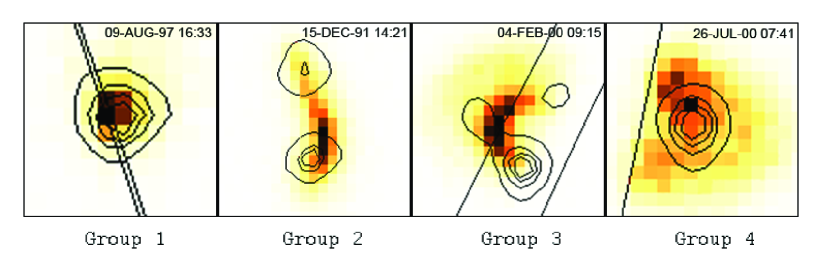
Figure 1: Examples of groups introduced in the text. The contours and the half-tones show the HXT/M1 and SXT/Be119 images, respectively. The pixel size is 2.45 arcsec². North is at the top, west – to the right.

For each flare from the list we computed one image at the peak count rate in the M1 band. To obtain an image of good quality we need about 200 counts per subcollimator, therefore we accumulated signal within a time interval of between 0.5 and 11 s (see column (7) in Table LABEL:113), depending on the total number of counts in the band M1. Next, we carefully defined the shape of the individual emission sources and combined the signal from all pixels inside each source separately. Due to the limited dynamic range of the HXT and the image reconstruction process, estimated to be about one decade (Sakao sakao (1994)), we considered as background the pixels having a signal below 10% of the brightest one. Sometimes emission sources in the M1 band were not well resolved, thus we calculated images in higher energy bands, if available, to define the border between the sources more precisely.

Keeping in mind that the loop-top and footpoint hard X–ray emission sources are a common characteristic of the impulsive phase of solar flares (e.g. Tomczak tomczak-occulted (2001)), we recognized four groups of events (see column (8) in Table LABEL:113):

• The group 1 (35 events) for which the HXT could not resolve individual sources.

• The group 2 (37 events) for which the HXT detected only footpoint sources.

• The group 3 (40 events) for which the HXT detected footpoint and loop-top sources.

• The group 4 (5 events) for which the HXT detected only loop-top sources.

Examples of events from each group are presented in Fig. 1. Events from group 1 are generally too small for the imaging capability of the HXT, thus we excluded them from further analysis. The presence of groups 2 and 4 is likely caused by the limited dynamic range of the HXT. For events from group 2, footpoint sources are brighter than the loop-top source by more than 10 times, opposite to events from group 4 for which the loop-top source is brighter than footpoint sources by more than 10 times. In both cases the fainter sources cannot be resolved from the background but we expect that they exist.

Following Petrosian et al. (petrosian2 (2002)) we define a parameter $\Re$ which is a ratio of the sum of the counts of the footpoint sources to that of the loop-top sources.

$$\Re=F_{FP}/F_{LT}$$ (1)

As a consequence, events from group 2 have values of $\Re$ greater than 10, events from group 4 have values of $\Re$ less than 0.1, and events from group 3 have values of $\Re$ between 10 and 0.1 (see column (9) in Table LABEL:113).

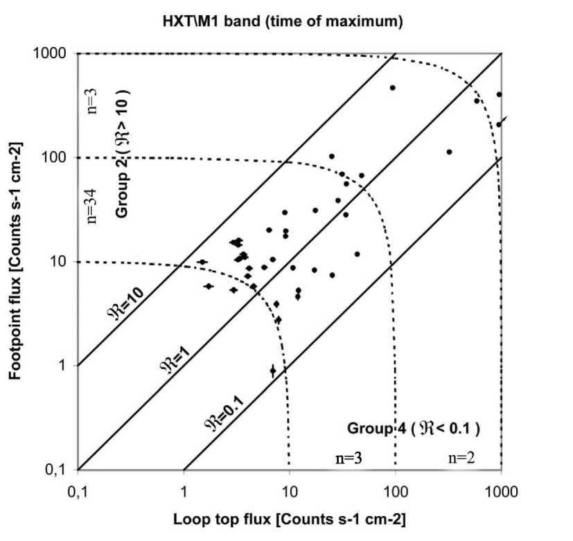
Figure 2: Counts from the footpoints versus loop-top counts in the HXT/M1 energy band for 40 flares of group 3. The diagonals represent lines of constant ratio $\Re$. The lines $\Re=10$ and $\Re=0.1$ establish detection thresholds of the instrument. Above the line $\Re=10$ we find the group 2 (37 events), below the line $\Re=0.1$, the group 4 (5 events). The dotted curves show lines of the constant total flux; the lowest one marks the event selection threshold.

In Fig. 2 we present a plot of the count rates of the footpoint source versus the count rates of the loop-top source for events from group 3. In the case of multiple-source events of the same class, coronal or chromospheric, we added their fluxes. It means that in this plot one flare is represented by one point. Error bars in Fig. 2 are statistical uncertainties, thus the actual uncertainties, including the possibility of contamination of one source by neighboring ones or an error of the reconstruction method, should be larger. The diagonals in Fig. 2 represent the line of equal fluxes ($\Re=1$) and detection thresholds arising from the finite dynamic range of the HXT. In this plot events from group 2 are located above the upper diagonal ($\Re>10$) and events from group 4 below the lower one ($\Re<0.1$).

The primary trend seen in Fig. 2 is an obvious correlation between fluxes of both classes of hard X–ray sources over three decades of flux. This trend mimics a ‘corridor’ between the diagonals $\Re=10$ and $\Re=0.1$ that constitutes an area where the HXT provides a reasonable detection of sources. Within the corridor a concentration of events rises as fluxes fall. An empty area in the lower left corner of the corridor is a truncation effect introduced by our selection criteria.

The second striking feature in Fig. 2 is an increase in flares for which footpoint sources are brighter than loop-top ones. Going from the left upper corner to the right bottom one in this figure we observe a continuous decrease in flare frequency: for 37 events $\Re$ is greater than 10, for 26, $\Re$ is between 10 and 1, for 14 events, between 1 and 0.1, and for 5 events, below 0.1. This decrease is independent of flux, therefore we conclude that this is not an artifact and must be intrinsic to the flare process, another than a global amount of released energy. Similar results were obtained by Petrosian et al. (petrosian2 (2002)), however the larger number of events in our sample allows us to discuss the different values of the parameter $\Re$ in solar flares.

Petrosian & Donaghy (petrosian (1999)) calculated spatial distributions of hard X–ray emission from flare loops assuming different values of parameters such loop length, field geometry of the loop, distribution of non-thermal electrons or plasma density within the loop. They found that in many cases the distribution is strongly dominated by footpoint sources because the emission mechanism is the most efficient there. However, they also obtained that an enhancement of emission from the loop-top is possible if at least one of the following conditions is fulfilled:

1. A pancake-type pitch-angle distribution of the accelerated electrons.

2. Scattering by plasma turbulence at the acceleration site.

3. Converging field geometry of the flare loop.

4. Strong increase of the column depth along the flare loop due to chromospheric evaporation.

The first two conditions refer to the acceleration process of non-thermal electrons in solar flares, the last two refer to the propagation process of non-thermal electrons within the flare loop. Generally, it is difficult to distinguish the influence of particular conditions with a reasonable confidence for individual events. However, we can estimate the general importance of converging field geometry and column depth along the flare loop for the ratio $\Re$ for a large sample of events.

The field convergence in the flare loop increases the pitch angle of the electrons as they descend. As a consequence, part of electrons can be reflected back by a magnetic mirror up to the loop-top before the transition region. Thus, the higher magnetic mirror ratio $M_{r}=B_{foot}/B_{top}$, the greater the trapping efficiency:

$$M_{r}=B_{foot}/B_{top}=1/{\sin}^{2}{\alpha}_{c}$$ (2)

where ${\alpha}_{c}$ is the critical value of pitch-angle (Aschwanden aschwssr (2002)). This means that all electrons having a pitch angle greater than ${\alpha}_{c}$ remain in the trap. Thus, an increase of the magnetic mirror ratio $M_{r}$ should decrease the hard X–ray flux ratio $\Re$ due to a decrease of electrons reaching the footpoints and an increase of electrons remaining in the loop-top.

For limb flares we cannot measure magnetic field strength directly. However, there is well-known relation between this parameter and height. Aschwanden et al. (1999a ) analyzed the three-dimensional coordinates of 30 loops from the Extreme-Ultraviolet Imaging Telescope (EIT) 171 Å image on 1996 August 30. They estimated the height dependence of the magnetic field $B(h)$ of the 30 potential field lines closest to the analyzed EIT loops and found that it can be approximated by a dipole model:

$$B(h)=B_{foot}{(1+\frac{h}{h_{D}})}^{-3},$$ (3)

where $h_{D}=75$ Mm is the mean dipole depth. We can rewrite this formula using the magnetic mirror ratio, $M_{r}$, definition:

$$M_{r}={(1+\frac{h}{h_{D}})}^{3}.$$ (4)

From Eqs. (2) and (4) we see that under the assumption of an isotropic pitch-angle distribution the height increase of the flare loop from 10 Mm to 20 Mm decreases the number of electrons reaching the footpoints by about 20% and increases the number of electrons remaining in the loop-top by about 33%. Therefore, we expect that a height dependence of the flux ratio of hard X–ray sources $\Re(h)$ should exist where $\Re$ drops as $h$ increases. This relation is independent of the energy of electrons.

The mean free-path of electrons $l_{f}$ in a volume having electron density $n_{e}$ can be estimated according to (Tsuneta et al. tsuneta_f (1997)):

$$l_{f}=8.3\times 10^{17}E^{2}/n_{e},$$ (5)

where $E$ is the electron energy in keV and $n_{e}$ is counted per cm^-3. Thus, in conditions typical of the pre-flare phase ($n_{e}\,{\sim}\,10^{9}{\div}10^{10}$ cm^-3), $l_{f}$ is greater than the loop semi-length. This means that almost all electrons accelerated at the top of the flare loop easily reach the transition region producing hard X–ray footpoint sources. An increase of electron density within the flare loop due to chromospheric evaporation limits the number of electrons that deposit their energy in the footpoints. As a consequence, the flux ratio of hard X–ray sources $\Re(h)$ should decrease as the column depth, $N=n_{e}L$, measured along the loop of the semi-length $L$, increases.

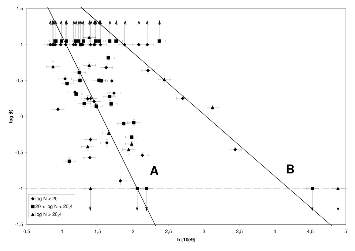
Figure 3: The ratio $\Re$ (on a logarithmic scale) versus the height of the flare loop for 82 events. For group 2 and 4 only the lower and upper approximation of $\Re$ is known, respectively. Different symbols denote different values of the column depth along the flare loop. A linear fit to the points from two branches is described by Eqs. (6) and (7).

Such relatively simply relationships $\Re(h)$ and $\Re(N)$ can become more complex if anomalous electron scattering occurs (Melrose melrose (1980)). This is caused by MHD turbulence which can be excited in the coronal segment of the flare loop by anisotropies occurring in the distribution of accelerated particles. Electrons with such a distribution can excite whistler waves. The MHD pitch-angle scattering is more effective than the Coulomb scattering and it pushes electrons with large pitch angles into the small pitch-angle regime. Thus, the anomalous scattering contributes to the footpoint yield electrons which would otherwise be mirrored high in the corona. The importance of this effect has been proved for energetic ions (Hua et al. hua (1989)) and for relativistic electrons (Miller & Ramaty miller (1989)). Recently, Karlický (karl2 (2005)) has shown that anomalous scattering can be important also for superthermal electrons.

To determine the relationships $\Re(h)$ and $\Re(N)$ we estimated values of $h$, $L$, and $n_{e}$ for flares from Table LABEL:113 using SXT images. The height, $h$, was directly measured in the Be119 images with a constant error of half of the SXT pixel i.e. about 0.9 Mm. Then, it was corrected for the projection effect by using flare heliocentric coordinates (column (4) in Table LABEL:113). We assumed a perpendicular orientation of loops relative to the solar surface. To verify our values we also measured the separation between footpoints and assuming circular loops we obtained an independent estimation of the height. Differences in obtained values of $h$ are considered as a measure of their uncertainty. Having $h$ we calculated the semi-length $L$ of the loop, $L=0.5{\pi}h$, assuming circular loops.

To estimate the electron density within the flare loop we chose a pair of SXT images taken with the filters Be119 and Al12 closest in time to the moment of peak maximum in the M1 band. We calculated values of temperature and emission measure averaged over the whole flare loop. To estimate the emitting volume we assumed the thickness of flare loop to be equal to its diameter ${\pm}0.5$ SXT pixel. Having the emission measure and volume we calculated the value of $n_{e}$, thus the column depth $N$. Obtained values of $h$ and $N$ are given in Table LABEL:113 in column (10) and (11).

For 21 events we could not calculate electron density due to a lack of useable SXT images for the maximum in the M1 band. As a substitute we adapted records from the Geostationary Environmental Operational Satellites (GOES). We used normalization coefficients for different satellites as well as recent coefficients for a polynomial approximation to the GOES temperature and emission measure response (White et al. goes (2005)). The obtained values of the column depth (see column (12) in Table LABEL:113) are systematically higher than those obtained by the SXT (by a factor 4, on average).

In Fig. 3 we present the relation between the flux ratio $\Re$ of hard X–ray sources on a logarithmic scale and the height for 40 flares for which we obtained values of $\Re$ of between 10 and 0.1. The points are concentrated along two branches which can be described by the following formulae:

$$\log{\Re}=(-2.05\pm 0.8)\times h+(3.2\pm 0.6)\quad\mbox{for 35 points}\quad$$ (6)

and

$$\log{\Re}=(-0.83\pm 0.15)\times h+(2.5\pm 0.4)\quad\mbox{for 5 points}\quad$$ (7)

In this figure we also plot the points that represent events of group 2 and 4 for which we know only a lower and upper approximation of $\Re$, respectively. Almost all points from these two groups are located along the same branches described with Eqs. (6) and (7). In column (13) in Table LABEL:113 we divide the events into branches. For 11 events from group 2 the branches are located too close to decide about the membership.

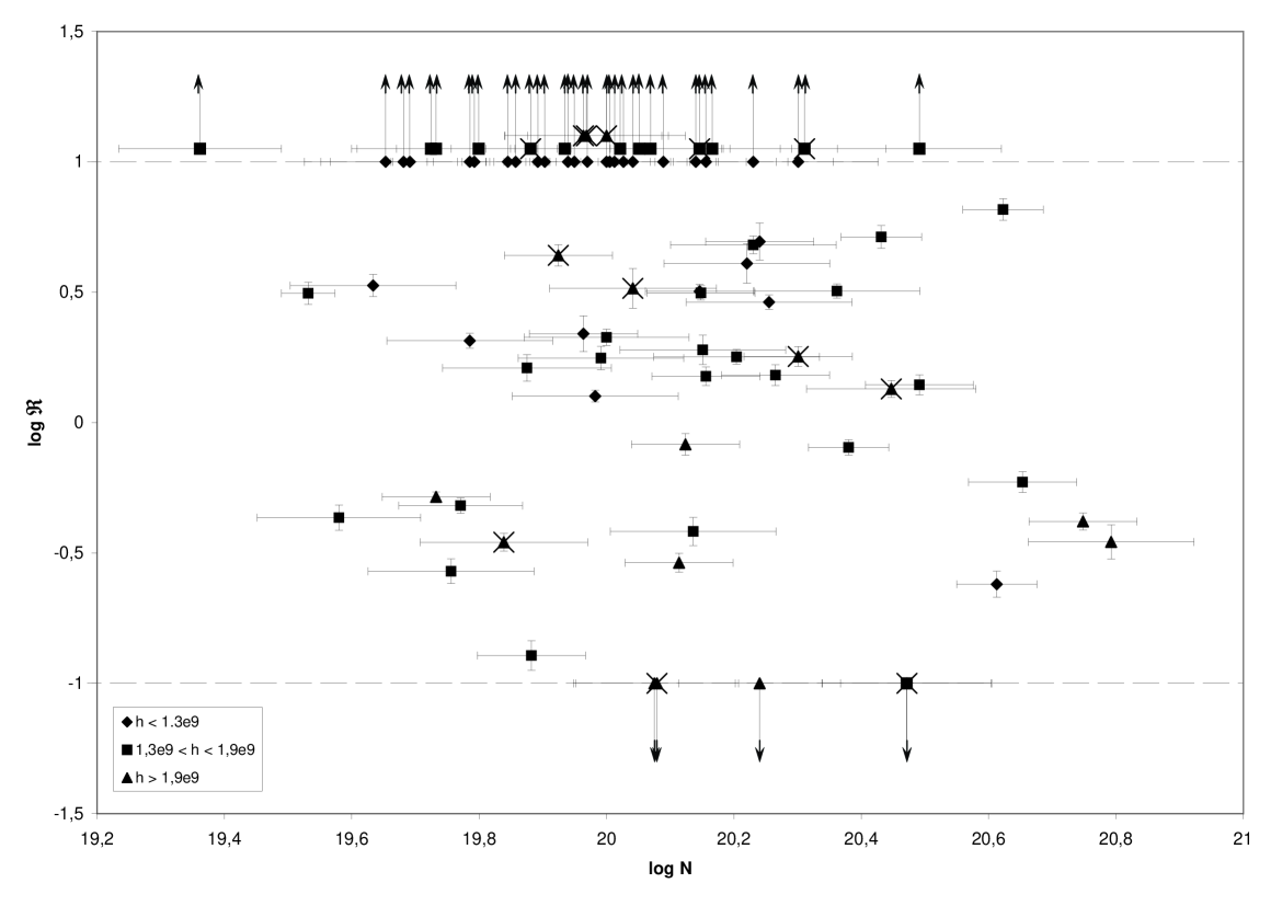
Figure 4: The ratio $\Re$ versus the column depth along the flare loop (both on a logarithmic scale) for 82 events. For group 2 and 4 only the lower and upper approximation of $\Re$ is known, respectively. Different symbols denote different values of the height of the flare loop. Events from the branch B in Fig. 3 are marked by crosses.

The scatter seen in Fig. 3 can be caused by different statistical as well as systematic factors. Unfortunately, we have no observational criteria that allow us to study the influence of the acceleration process of non-thermal electrons in solar flares on the ratio $\Re$. To separate the influence of the column depth on the height dependence of the ratio $\Re$ we introduce three symbols: diamonds, boxes, and triangles, which refer to events with lower ($<1.0{\times}10^{20}$ cm^-2), intermediate, and higher ($>2.4{\times}10^{20}$ cm^-2) column depth. In this figure we used the more complete set of data including the column depths estimated from GOES data. As we see, different values of the column depth are not responsible for the separation between the two branches in Fig. 3 because different symbols are present in both branches.

In Fig. 4 we show the relation between the flux ratio $\Re$ of hard X–ray sources and the column depth, both on a logarithmic scale, for the 40 flares for which we obtained values of $\Re$ between 10 and 0.1 and estimated the column depth. In this figure we also plot the points that represent events of group 2 and 4 for which we know only the lower and upper approximation of $\Re$, respectively. We used the more complete set of data including the column depth estimated from GOES data. No correlation is seen, even if we plot SXT data instead of GOES ones.

To determine the influence of the height on the column-depth dependence of the ratio $\Re$ we introduce three symbols: diamonds, boxes, and triangles which refer to events with lower ($<$13 Mm), intermediate, and greater ($>$19 Mm) height. The different symbols in Fig. 4 are distributed almost uniformly within the range of values of $N$ which suggests that the influence of height is not responsible for the lack of dependence between the ratio $\Re$ and the column depth.

4 Discussion

We expected that both $\Re(h)$ and $\Re(N)$ could be detected using Yohkoh data despite the complex interaction between many parameters and the relatively high values of their uncertainties. Our analysis confirms the existence of the $\Re(h)$ relationship only.

4.1 $\Re(h)$ dependence

We found that the ratio $\Re$ decreases as the height of the flare loop rises, however, this relationship is complex with two branches: a left, steeper, and a right, flatter. We excluded different values of the column depth as the cause of the membership of a particular branch. We do not think that the acceleration process of non-thermal electrons decides into which branch the event falls. If so, then all points from the branch B in Fig. 3 should have a particular distribution of electrons which makes propagation into the footpoints more efficient than for other events. Thus, the points from the branch B in Fig. 3 should also show higher values of the ratio $\Re$ for similar values of the column depth in Fig. 4. These points are marked by crosses and as we see, this is not the case.

We suggest that events from different branches in Fig. 3 occurred in magnetic loops having different converging field geometries. Thus, events from branch A occurred in more converged loops than the events from branch B. This is confirmed by the different inclination of the branches. For the branch A an increase of the height of about 9.5 Mm, on average, transforms the flux ratio $\Re$ from the value of 10 into the value of 0.1, i.e. it makes the event of group 4 instead of the event of group 2. To do the same for the branch B an increase of height of about 24 Mm is needed.

We used our data to estimate the frequency of occurrence of more-converged and less-converged loops in the solar corona. We have classified 58 events into branch A and 13 events into branch B (see column (13) in Table LABEL:113). This gives an 82% contribution of the more-converged loops and an 18% contribution of the less-converged ones. For group 2 the branches are situated very close each to other, therefore a safer method is to take into account only events of group 3 and 4. In this case the contribution of the more-converged loops is even higher (38 events of 45 i.e. 84%) and the contribution of the less-converged ones is 16% (7 events of 45).

Figure 5: Changes of the magnetic mirror ratio against the height of the magnetic loop calculated with formula (4). Different values of the mean dipole depth, $h_{D}$, reflect different inclinations of the branches A and B in Fig. 3.

To describe the convergence of the investigated magnetic loops more quantitatively we used formula (4) and assumed a priori that it works for more frequent events from branch A (Fig. 5). We calculated the magnetic mirror ratio, $M_{r}$, for terminal heights, 11 and 20.5 Mm, establishing the group 3 for branch A. The obtained values of $M_{r}$ are 1.51 and 2.06, respectively. This means that an increase of the magnetic mirror ratio by a factor 1.36 completely changes the spatial distribution of hard X–ray emission in solar flares. For $M_{r}\leq 1.51$ the population of electrons reaching the footpoints is so large that the HXT can detect only footpoint sources. For $M_{r}\geq 2.06$ the population of electrons trapped around the loop-top is so large that the HXT can detect only loop-top sources.

If our explanation is consistent, the magnetic loops from branch B should reach the same values of $M_{r}$, 1.51 and 2.06, for greater terminal heights, 18 and 42 Mm, respectively. To fulfil this condition the mean dipole depth, $h_{D}$, in formula (4) should increase to 138$\pm$16 Mm i.e. by a factor 1.8 (Fig. 5).

Our results are consistent with Aschwanden et al. (aschw-batse (1998)) who estimated the magnetic mirror ratio for 46 solar flares recorded by the Burst and Transient Source Experiment (BATSE) onboard the Compton Gamma Ray Observatory (CGRO). For a comparison see Table 1.

The observed width variation of coronal loops has been extensively investigated due to its ability to test magnetic field models in the solar corona. Many authors have measured the ratio of the loop diameter at the top to that at the footpoint, the so-called expansion factor, for selected magnetic loops observed by different instruments: Yohkoh/SXT, SoHO/EIT, TRACE (Klimchuk et al. klim1 (1992), Aschwanden et al. 1999a , Klimchuk klim2 (2000), Watko & Klimchuk klim3 (2000), Khan et al. khan (2004), López Fuentes et al. lopez (2006)). Different sets of non-flare and post-flare loops gave average values of the expansion factor between 1.0 and 1.3. The authors did not report any tendency towards loop differentiation for separate values of the expansion factor. Moreover, Watko & Klimchuk (klim3 (2000)) did not find any correlation between the expansion factor and loop length.

Our results are different. First, we found the relation $\Re(h)$ which we interpret as a consequence of a correlation between the expansion factor and the loop length. Second, we identified two kinds of converging field geometry (the branches A and B in Fig. 3). Third, many of the investigated events suggest an expansion factor above the upper limit of previous investigations. However, we developed a new method to estimate the expansion factor of loops in which non-thermal electron beams are used as a diagnostic tool. This method includes the convergence of loops at the entrance into the chromosphere in a better way than a direct measure of the loop diameter ratio because of the limited sensitivity of SXR and EUV filters due to the temperature decrease.

Table 1: Comparison between estimations of the magnetic mirror ratio for flares investigated by Aschwanden et al. (aschw-batse (1998)) and in this paper.

	Number of events
Magnetic mirror	Aschwanden et al.	This paper
ratio $M_{r}$	(aschw-batse (1998))
$\leq$1.5	21 (45.6%)	37 (45.1%)
1.5–2.1	17 (37.0%)	40 (48.8%)
$\geq$2.1	8 (17.4%)	5 (6.1%)
Total	46 (100%)	82 (100%)

Conventional magnetic field models, including a potential or a force-free extrapolation of photospheric magnetograms, predict that the expansion factor should be much larger than those obtained from observations (Aschwanden aschwpodr (2004)). To explain the discrepancy between the observed and expected expansion it has been postulated that magnetic flux tubes that correspond to observed plasma loops are current-carrying and a helically twisted (Klimchuk et al. klim4 (2000)). Such flux tubes show a reduced expansion factor due to the magnetic tension associated with the azimuthal field component that is introduced by the twist.

To understand what differentiates the investigated flare loops in Fig. 3, we applied a interpretation of helically twisted flux tubes (Klimchuk et al. klim4 (2000)). In this picture the more-converged loops from branch A in Fig. 3 correspond to flux tubes that are less twisted, and the less converged loops (the branch B in Fig. 3) correspond to flux tubes that are more twisted.

To verify this hypothesis we considered three observables which may depend on the helical twist of the flux tube in which the flare occurred. They are: (1) temperature of the flare, (2) magnetic complexity of the active region, and (3) the connection with Coronal Mass Ejections (CMEs). However, none have shown any systematic difference between events from branch A and B. A lack of a difference probably means that the connection between the observables and the helical twist of the flux tube is too loose and is missed due to observational uncertainties. A further search for a more convenient observable representing the helical twist is needed.

When discussing the possibility of the occurrence of two types of magnetic loops, the more converged and less converged, the same loop can show a different convergence in its footpoints. Such a solution was proposed by Sakao (sakao (1994)) to explain the asymmetry of footpoint hard X–ray emission sources in five disc flares. He found that usually the brighter source is co-spatial with an area where the magnetic field is fainter. He concluded that due to a lower convergence in this footpoint, non-thermal electrons precipitate deeper where hard X–ray photons are produced more efficiently. Based on microwave images, Kundu et al. (kundu (1995)) confirmed this for two other flares. In this case the brighter footpoint source was co-spatial with an area of a stronger magnetic field due to the dependence of microwave emission on magnetic field intensity.

If Sakao’s scheme is correct then the stronger asymmetry of convergence in the flare loop causes the stronger asymmetry of hard X–ray emission. As a consequence, the flux ratio $\Re$ depends more strongly on properties of the brighter, less-converged footpoint. Thus, the membership of events of the branch B in Fig. 3 might be caused by the magnetic configuration in which only the one footpoint is less converged.

Table 2: Values of the asymmetry ratio $a$ for events from branch A and B.

Branch	$a\leq 0.67$	$a>0.67$
A (55 events)	22 (40%)	33 (60%)
B (11 events)	4 (36%)	7 (64%)
Total (66 events)	26 (39%)	40 (61%)

To verify this possibility we compared the asymmetry of footpoint sources of events from branch A to those from branch B for events from groups 2 and 3. Following Aschwanden et al. (1999b ) we defined the asymmetry ratio $a$ of the footpoint hard X–ray fluxes $F_{FP1}$ and $F_{FP2}$:

$$a=\frac{F_{FP2}}{(F_{FP1}+F_{FP2})},\quad\mbox{where}\quad F_{FP1}<F_{FP2}.$$ (8)

With this definition, the asymmetry ratio varies from $a=0.5$ for symmetric footpoints to $a=1$ for the one-sided footpoint. We found that about 40% of events show small values of the asymmetry ratio ($a\leq 0.67$) and about 60% of events show large values of the asymmetry ratio ($a>0.67$). The contribution of symmetric and asymmetric events in both branches is almost the same (see Table 2). Thus, asymmetric convergence in flare loop footpoints can influence the location of events in the $\Re$–$h$ diagram, however, it does not explain the division into two branches.

Goff et al. (goff (2004)) have shown that a different brightness in flare footpoint hard X–ray sources also can be caused by a non-central location of the acceleration site in the magnetic loop. For many events we could not precisely localize the acceleration site, therefore we did not discuss this possibility.

Employing the effect of anomalous electron scattering in the flare loop it is possible to give an alternative explanation for presence of two branches in Fig. 3: all investigated events show a similar convergence but in the case of flares from branch B the anomalous electron scattering operates in an opposite way to events in branch A. This effect decreases values of the pitch angle of electrons, therefore for the same height we should observe a higher value of the ratio $\Re$. Unfortunately, the HXT has a poor energy resolution so we could not verify the status of the electron scattering.

4.2 $\Re(N)$ dependence

Opposite to our expectation we have not found any correlation between the flux ratio $\Re$ and the column depth $N$ along the flare loop (see Fig. 4). A reason for this may be the time interval chosen for analysis — the maximum in the HXT/M1 energy band. It may be too early for efficient operating of the chromospheric evaporation. This explanation is supported by the fact that in Fig. 4 the values of $\Re$ less than 1 do not occur for short loops ($h<$ 13 Mm) with the only exception of the strong flare of August 18, 1998 (event No. 49).

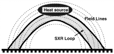
Figure 6: Reproduced from Hori et al. (hori (1997)). Field lines connecting a heat source and footpoints extend outside the bright loop seen in soft X-rays which is an apparent product of successive energy release and inertia of the chromospheric evaporation.

The lack of correlation in Fig. 4 can be explained also by the scheme presented in Fig. 6. This figure is reproduced from Hori et al. (hori (1997)). As we see, field lines connecting a heat source and footpoints extend beyond the bright loop seen in soft X-rays. The impression that we observe a single bright loop was caused by successive energy release from the innermost loop to the outermost and the inertia of chromospheric evaporation. If this scheme is correct we should rather measure the column depth outside the bright legs seen in SXT images which apparently connect the loop-top and footpoint hard X–ray sources. The scheme from Fig. 6 does not need to work for each of the investigated events to argue against a correlation between the flux ratio and the column depth. Anomalous electron scattering can be an additional cause that makes the correlation between $\Re$ and $N$ unclear.

5 Conclusions

We investigated the spatial distribution of hard X–ray emission in solar flares. We concentrated on the relationship between the loop-top and footpoint emission sources. In comparison to previous studies (Masuda masuda (1994), Petrosian et al. petrosian2 (2002)) the list of investigated flares is more complete (117 events instead of 10 or 18, respectively) due to the mission-long Yohkoh/HXT database that was included and the more liberal selection criteria that were used.

We investigated the dependence of the flux ratio $\Re$ of the footpoint and loop-top sources on other observational parameters like the flare loop height $h$ and the column depth $N$ along the flare loop. We found a clear correlation between $\Re$ and $h$ (Fig. 3) which we interpret as an effect of converging field geometry. Since this correlation is stronger than other parameters and observational uncertainties we conclude that the influence of magnetic convergence on the spatial distribution of hard X–ray emission in solar flares is the strongest, at least under conditions defined in this investigation i.e during the early phase of the flare evolution. This is confirmed, to some extent, by the lack of any correlation between the flux ratio $\Re$ and the column depth $N$ (Fig. 4). However, this can be also caused by a more complex configuration of investigated events than is seen in soft X–rays (see Fig. 6).

Using the formula from Aschwanden et al. (1999a ) we developed a new method of calculating the magnetic mirror ratio in solar flare loops using non-thermal electron beams as a diagnostic tool for magnetic convergence. The obtained values of the magnetic mirror ratio are consistent with previous results and suggest a nonpotential configuration strongly distorted by the presence of longitudinal currents.

The two branches seen in the $\Re-h$ diagram suggest that in the solar corona two kinds of magnetic loops can exist: a more converged kind that is more frequent (above 80%) and a less converged kind that is less frequent (below 20%). In a dipole approximation the mean dipole depth $h_{D}$ differs between the branches by a factor of 1.8, on average. Despite the observed dichotomy in solar flare loops into more converged and less converged cases, we have no independent proof confirming such a division. Therefore, we cannot conclude, whether the division is real or random. Finally, what is a role of the anomalous electron scattering? Further studies are needed including more and better observed flares to answer these questions. For this, the Reuven Ramaty High-Energy Solar Spectroscopic Imager (RHESSI) is ideal due to its dynamic range and energy resolution better than the HXT. This work is in progress.

We hope that further study will allow us to understand also the concentration in the rarely-occupied branch B in Fig. 3 of many known and extensively investigated flares e.g. of January 13, 1992 (Masuda et al. masuda-nat (1994)), of February 17, 1992 (Doschek et al. doschek (1995)), of June 28, 1992 (Tomczak tomczak-pajak (1997)), and of October 4, 1992 (Masuda et al. masuda-pasj (1995)).

Table 3: List of selected flares (^a Values in parenthesis are estimated from SXT images; ^b M – Masuda masuda (1994), P – Petrosian et al. petrosian2 (2002)).

No.	Date	GOES	Disk	NOAA	M1	Time	Group	$\Re$	$h$	$N$ [1020 cm-2]		Branch	Rem.b
		class	positiona	AR	cts.	interval			[Mm]	SXT	GOES	[Fig. 3]
(1)	(2)	(3)	(4)	(5)	(6)	(7)	(8)	(9)	(10)	(11)	(12)	(13)	(14)
1	91/11/09	M1.4	S14W69	6906	105	20:52:09+2	2		15	0.34	1.4	?
2	91/11/17	M1.9	S12E78	6929	49	18:33:17+2	2		10	0.20	1.7	A
3	91/12/02	M3.6	N16E87	6955	24	04:53:44+4.5	3	0.48	14	0.21	0.59	A	M, P
4	91/12/03	X2.2	N17E72	6955	1297	16:36:30+0.5	1		12	0.79	2.2
5	91/12/07	C6.4	N09E72	6961	17	21:52:46+7.5	1		12	0.52	0.27
6	91/12/08	M2.6	N08E65	6961	12	07:35:00+9	1		15	0.61	0.92
7	91/12/09	M1.1	S06E88	6966	13	18:53:46+9.5	3	6.6	17	0.31	4.1	A
8	91/12/15	C6.0	S12E76	6972	14	14:21:42+5	2		12	0.20	0.62	A	M, P
9	91/12/16	C7.8	S10E69	6972	43	03:13:06+2.5	2		10	0.27	0.80	A
10	91/12/16	M1.6	S12E67	6972	50	06:38:15+2.5	2		9	1.4	1.4	A
11	91/12/18	M3.5	S10E88	6980	106	10:27:30+1.5	3	1.4	15	0.31	3.1	A	M, P
12	92/01/13	M2.0	S16W86	6994	29	17:28:11+3.5	2		24	0.11	0.93	B	M, P
13	92/02/06	M7.6	N05W82	7030	144	03:23:50+1	4		22	0.38	1.7	A	M, P
14	92/02/17	M1.9	S16W81	7050	21	15:40:54+5	2		17	0.16	0.63	B	M, P
15	92/02/19	M3.7	N04E85	7067	17	03:48:23+6.5	3	4.4	22	0.23	0.84	B
16	92/02/26	M1.3	S16W90	7073	15	01:37:58+6.5	2		12	0.33	2.0	A
17	92/04/01	M2.3	S04E86	7123	38	10:13:04+3	2		9	0.64	1.0	A	M, P
18	92/04/19	C3.9	N04E85	7138	16	02:11:11+6.5	2		22	0.11	0.92	B
19	92/06/26	C2.9	N08W82	7205	11	12:52:15+9.5	1		9	0.26	0.97
20	92/06/28	M1.6	N10W89	7216	17	13:56:43+5.5	4		45		1.1	B
21	92/08/11	M1.4	(S15E81)	7260	77	22:25:20+1.5	1		14	0.19	0.42
22	92/09/09	M3.1	S09W71	7270	32	02:10:29+3.5	1		16	0.27	1.7
23	92/09/09	M1.9	S11W78	7270	15	17:58:33+6	1		14	0.17	1.5
24	92/10/04	M2.4	S05W90	7293	30	22:19:07+3	2		19	0.91	1.4	B	M, P
25	92/10/11	C8.3	S16W68	7301	14	02:03:36+10.5	2		15	0.14	0.54	?
26	92/11/05	M2.0	S17W84	7323	36	06:19:22+3	1		10	0.40	1.0		M, P
27	92/11/22	M1.6	N11E76	7348	31	23:07:49+4	2		9	0.73	0.61	A
28	92/12/04	M1.4	N19W71	7352	47	11:38:32+2	2		15	0.31	0.86	?
29	93/02/05	C7.7	S07E78	7420	29	07:53:38+3.5	1		15		0.55
30	93/02/06	C5.6	S08E66	7420	23	05:25:56+4.5	1		8		0.90
31	93/02/14	M2.0	S22E78	7427	53	12:53:04+3	1		14	0.50	2.3
32	93/02/17	M5.8	S07W87	7420	94	10:36:21+1	3	2.2	12	0.22	0.92	A	M, P
33	93/02/21	M1.4	N13E75	7433	14	00:39:35+8.5	3	2.9	11	0.60	1.8	A
34	93/03/15	C3.0	N06W88	7411	15	09:59:44+9	2		12	0.11	0.92	A
35	93/06/11	C5.7	S13W80	7518	12	10:14:59+9.5	3	0.35	34		0.69	B
36	93/06/25	M5.1	(S09E90)	7530	17	03:18:23+6	3	1.5	13	0.22	1.4	A
37	93/09/27	M1.8	(N09E89)	7590	41	12:08:14+4.5	2		9	0.62	1.1	A	P
38	93/10/09	M1.1	N11W78	7590	11	08:08:18+10	3	3.4	10	0.25	0.43	A
39	93/11/30	C9.2	(N19E84)	7618	70	06:03:31+4	2		14	0.21	1.0	?	P
40	94/01/16	M6.1	N09E70	7654	57	23:17:27+2	3	0.83	20	0.51	1.3	A
41	94/01/17	C9.3	N06E65	7654	12	09:14:49+10.5	2		15	0.16	1.2	?
42	97/08/09	C8.5	N19W85	8069	12	16:33:35+10	1		9		1.4
43	97/09/14	C2.8	S23W79	8083	17	02:53:26+6	2		15		0.23	?
44	97/11/15	M1.0	N20E65	8108	15	22:42:04+5.5	4		49		3.2	B
45	98/05/08	M3.1	(S16W90)	8210	48	01:57:35+2	3	1.8	14	0.19	1.6	A	P
46	98/05/28	C8.7	(N16W89)	8226	12	19:02:55+10	3	2.1	12	0.15	0.61	A
47	98/08/14	M3.1	S23W74	8293	65	08:25:57+2	1		10	1.4	2.2
48	98/08/18	X2.8	(N34E85)	8307	599	08:20:29+0.5	4		14	1.1	3.1	A	P
49	98/08/18	X4.9	N33E87	8307	2819	22:16:40+0.5	3	0.24	11	1.2	4.1	A	P
50	98/09/02	M2.2	(N18W82)	8319	20	17:03:50+5	2		13	0.35	0.48	?
51	98/09/28	C9.5	(S14W90)	8342	26	12:00:22+4.5	2		9	0.20	1.4	A
52	98/09/28	C6.8	(S14W90)	8342	21	16:08:14+5.5	2		9	0.17	0.45	A
53	98/11/09	C4.9	N22W70	8375	21	21:12:21+5.5	3	4.8	16	0.20	1.7	A
54	98/11/10	C7.9	N20W76	8375	51	00:12:25+2	1		11	0.64	1.3
55	98/11/10	C3.3	N21W76	8375	18	06:52:25+6	1		12	0.77	4.0
56	98/11/10	M1.8	N21W78	8375	56	15:42:44+2	1		15	0.23	2.0
57	98/11/11	M1.0	N22W86	8375	18	04:05:54+6	3	3.2	15	0.62	2.3	A
58	98/11/11	C3.5	N22W90	8375	13	07:36:32+10	1		14	0.28	0.85
59	98/11/22	X3.7	S29W80	8384	1200	06:39:38+0.5	3	0.42	20	0.86	5.6	A
60	98/11/22	X2.5	S29W86	8384	830	16:20:42+0.5	3	0.59	17	1.6	4.5	A
61	98/11/23	C4.9	(S30W89)	8386	14	05:58:55+9.5	3	0.51	20	0.11	0.54	A
62	98/11/24	C8.4	N19E77	8395	18	22:12:33+6.5	2		12	0.12	1.0	A
63	98/11/25	C6.4	(N19E69)	8395	14	14:01:01+9.5	2		8	0.30	0.87	A
64	99/01/14	M3.0	(N20E65)	8460	12	10:14:42+9.5	1		21		2.0
65	99/06/20	C5.5	(N16E90)	8594	18	08:36:24+7	3	5.2	14	0.10	2.7	A
66	99/08/04	C5.4	S22W70	8645	14	23:33:52+9	1		12	0.27	0.87
67	99/08/20	C7.8	S23E66	8674	21	19:22:44+5.5	2		11	0.40	1.2	A
68	99/09/01	C6.6	S28W76	8674	27	18:56:25+4	2		21	0.19	0.76	B
69	99/09/19	C9.6	N20W77	8699	13	23:06:39+9	3	1.8	27	0.19	0.98	B
70	99/10/26	M3.7	(S15W88)	8737	18	21:21:33+7	3	0.80	19	0.42	2.4	A
71	99/10/27	M1.0	S12W89	8737	12	09:09:48+11	1		10	0.79	1.1
72	99/11/07	C3.1	(N10E83)	8759	15	07:35:22+8	3	1.5	17	0.07	1.8	A
73	99/11/27	X1.4	S15W68	8771	351	12:11:09+0.5	1		13	1.6	3.2
74	99/12/03	C6.3	N13E80	8788	19	19:51:22+5.5	2		9	0.54	1.0	A
75	99/12/18	M1.5	N20E66	8806	259	19:11:51+0.5	2		14	0.76	3.1	?
76	00/02/04	M3.0	N27E79	8858	119	09:15:09+1	3	4.1	12	0.33	1.7	A
77	00/02/19	C4.5	S19W81	8878	13	06:17:02+10	1		13	0.18	0.52
78	00/03/07	M1.0	(S16E88)	8902	28	19:47:56+3.5	1		10	0.23	1.8
79	00/03/07	C8.7	S15E84	8902	170	21:55:45+1	2		10	0.09	0.48	A
80	00/03/27	C8.4	S09W69	8926	37	13:59:04+2.5	1		10	0.49	0.78
81	00/05/11	C3.6	S15E84	8998	11	22:23:17+10.5	1		8	0.30	0.96
82	00/05/15	M1.2	S20W66	8993	22	18:01:00+6	1		12	0.71	1.0
83	00/05/23	C4.3	S22W76	8996	26	17:50:15+4.5	1		11	0.31	1.0
84	00/06/01	M2.5	N19E80	9026	83	06:12:02+1.5	3	1.6	15		0.75	A
85	00/07/01	M1.5	N11W85	9054	14	23:23:14+9.5	3	3.2	16	0.20	1.4	A
86	00/07/13	C9.8	N17W77	9070	23	07:00:45+5	1		8	0.85	2.9
87	00/07/13	M1.5	N16W84	9070	42	22:03:38+2.5	1		10	0.91	2.0
88	00/07/14	M1.5	(N17W83)	9070	66	00:43:17+2	1		18	0.61	4.6
89	00/07/26	M1.3	(S20W90)	9087	18	07:41:57+6.5	4		21	0.36	1.2	A
90	00/07/27	M2.4	N12W71	9090	65	04:08:16+1.5	2		12	1.1	1.0	A
91	00/07/27	M1.5	(S11W90)	9091	18	16:47:57+7	3	0.43	16		0.38	A
92	00/09/30	X1.2	(N07W90)	9169	502	23:19:29+0.5	3	4.9	9	0.58	1.7	A
93	00/10/01	M2.2	(N07W90)	9169	52	14:00:38+2	3	1.9	17	0.34	1.4	A
94	00/10/14	M1.1	N04W82	9182	16	08:36:39+6	3	0.38	14	0.34	1.4	A
95	00/10/16	C7.0	(N04W90)	9182	26	05:42:54+4.5	3	3.1	17	0.06	0.34	A
96	00/10/28	C9.7	N15E83	9212	10	07:07:25+10	3	0.13	18	0.24	0.75	A
97	00/12/06	M1.6	(S11W66)	9246	12	22:25:21+11	3	1.8	14	0.62	2.0	A
98	01/01/25	C7.4	N10E73	9325	12	07:11:20+9	2		9	0.41	0.70	A
99	01/03/21	M1.8	(S06W66)	9373	12	02:35:12+10	3	1.3	9	0.59	0.96	A
100	01/03/21	C9.8	S07W70	9373	34	11:25:12+4	2		11		0.87	A
101	01/04/02	X20	(N16W70)	9393	394	21:36:16+0.5	3	0.35	19	2.3	6.2	A
102	01/04/04	C6.4	(N15W89)	9393	28	03:47:21+4	3	2.1	17		1.0	A
103	01/04/05	M3.1	(N14W90)	9393	65	02:07:37+2	3	1.4	31		2.8	B
104	01/04/05	M8.4	(N14W90)	9393	27	08:48:59+4	2		18	0.68	2.0	B
105	01/06/30	C6.0	N05E78	9562	15	20:41:07+9.5	2		13		0.72	?
106	01/08/28	C6.1	N15E81	9600	48	02:00:49+2	2		15		1.1	?
107	01/09/03	M2.5	(S23E88)	9605	18	18:23:23+7	2		12		0.78	A
108	01/09/13	C3.7	S11E73	9616	19	00:36:50+5.5	1		10		0.90
109	01/09/30	M1.0	S21W72	9628	38	11:34:26+2	3	3.3	24		1.1	B
110	01/10/01	M9.1	(S20W89)	9628	53	05:11:42+2	3	0.27	14		0.57	A
111	01/10/01	M1.2	(S17W77)	9632	39	23:43:56+2.5	1		12		1.6
112	01/10/02	C4.7	(S20W90)	9632	21	17:12:16+4	2		15		0.53	?
113	01/10/29	M1.3	(N12W88)	9673	18	01:56:32+6	3	3.2	13	0.53	1.4	A
114	01/11/01	M1.3	(S19E86)	9687	28	06:50:36+3.5	3	0.29	21	0.14	1.3	A
115	01/11/06	C5.6	S16E75	9690	35	01:31:15+3	1		9	0.40	1.4
116	01/11/06	M1.2	S17E74	9690	19	06:24:16+5	1		19	0.23	1.4
117	01/11/06	C9.0	S17E73	9690	10	09:28:16+10	1		10	0.71	2.3