The Structure and Dynamics of GRB Jets

Abstract

There are several lines of evidence which suggest that the relativistic outflows in gamma-ray bursts (GRBs) are collimated into narrow jets. The jet structure has important implications for the true energy release and the event rate of GRBs, and can constrain the mechanism responsible for the acceleration and collimation of the jet. Nevertheless, the jet structure and its dynamics as it sweeps up the external medium and decelerates, are not well understood. In this review I discuss our current understanding of GRB jets, stressing their structure and dynamics.

gamma rays: bursts hydrodynamics ISM: Jets and outflows relativity

0.1 Introduction

Gamma-ray bursts (GRBs) are produced by a highly relativistic outflow from a compact source (for a comprehensive recent review see Piran, 2005). Early GRB models featured a spherical outflow, mainly for simplicity. However, other astrophysical sources of relativistic outflows such as active galactic nuclei and micro-quasars are in the form of narrow bipolar jets. One might argue (e.g., Rhoads, 1997) that, in analogy to other such sources, GRBs might also be collimated into narrow jets.

The initial Lorentz factor during the prompt gamma-ray emission is very high, $\Gamma_{0}\gtrsim 100$, and therefore we observe emission mainly from very small angles, $\theta\lesssim\Gamma_{0}^{-1}\lesssim 10^{-2}\;$rad, relative to our line of sight. This is a result of relativistic beaming (i.e. aberration of light), an effect of special relativity, which causes an emission that is roughly isotropic in the rest frame of the emitting fluid (as is generally expected under most circumstances) to be concentrated mostly within an angle of $\Gamma^{-1}$ around its direction of motion in the lab frame, where $\Gamma\gg 1$ is the Lorentz factor of the emitting fluid in the lab frame. For this reason, the prompt gamma-ray emission probes a region of solid angle $\sim\pi\Gamma_{0}^{-2}$, or a fraction $\sim\Gamma_{0}^{-2}/4\sim 10^{-7}-10^{-4.5}$ of the total solid angle, and cannot tell us whether the outflow occupies a larger solid angle.

Therefore, more direct evidence in favor of jets in GRBs had to await the discovery of afterglow emission in the X-ray (Costa et al., 1997), optical (van Paradijs et al., 1997), and radio (Frail et al., 1997), that lasts for days, weeks, and months, respectively, after the GRB. The afterglow is believed to be synchrotron emission from the shocked external medium. As the relativistic outflow expands outwards it sweeps up the surrounding medium and drives a strong relativistic shock into it, called the forward shock, while the ejecta are decelerated by a reverse shock. Eventually, most of the energy is transfered to the shocked external medium behind the forward shock, and the flow approaches a spherical self-similar evolution (Blandford & McKee, 1976), gradually decelerating as it sweeps up the external medium.

This is valid not only for an initially spherical outflow, but also for the interior of a jet with an angular size larger than $\Gamma_{0}^{-1}$ (as appears to be the case for GRB jets, e.g. Panaitescu & Kumar, 2002), as long as $\Gamma^{-1}$ remains smaller than the angular size of the jet and the interior of the jet is out of causal contact with its edges (i.e. before the jet break time). Therefore, before the jet break time the isotropic equivalent energy of the jet, $E_{\rm iso}$, is relevant (both for its dynamics and for the resulting emission), while at very late times as the jet becomes sub-relativistic and approaches spherical symmetry its true energy, $E$, is relevant. In the intermediate regime things are more complicated, and are discussed in this review.

The forward shock is responsible for the long lived afterglow emission, while the reverse shock produces a shorter lived emission, that peaks in the optical or NIR on a time-scale of tens of seconds, when the reverse shock crosses the shell of ejecta (the “optical flash”, e.g. Akerlof et al., 1999; Sari & Piran, 1999a, b; Mészáros & Rees, 1999). The shocked outflow gradually cools adiabatically and the peak of its emission shifts to lower frequencies, until after about a day it peaks in the radio (the “radio flare” Kulkarni et al., 1999b; Frail et al., 2000; Berger et al., 2003a). During the afterglow, the Lorentz factor $\Gamma$ of the emitting shocked external medium decreases with time as it accumulates more mass, causing the visible region of $\theta\lesssim\Gamma^{-1}$ around the line of sight to increase with time. This enables us to probe the structure of the outflow over increasingly larger angular scales.

Different lines of evidence suggest that the relativistic outflows in GRBs are collimated into narrow jets. A compelling, although somewhat indirect, argument comes from the very high values for the energy output in gamma rays assuming isotropic emission, $E_{\rm\gamma,iso}$, that are inferred for GRBs with known redshifts, $z$, which approach and in one case (GRB 991023) even exceed $M_{\odot}c^{2}$. Such extreme energies in an ultra-relativistic outflow are hard to produce in models involving stellar mass progenitors. If the outflow is collimated into a narrow jet (or bipolar jets) that occupies a small fraction, $f_{b}\ll 1$, of the total solid angle, then the strong relativistic beaming due to the very high initial Lorentz factor ($\Gamma_{0}\gtrsim 100$) causes the emitted gamma rays to be similarly collimated. This reduces the true energy output in gamma rays by a factor of $f_{b}^{-1}$ to $E_{\gamma}=f_{b}E_{\rm\gamma,iso}$, thus significantly reducing the energy requirements.

Estimates of the energy in the afterglow shock from late time radio observations when the flow is only mildly relativistic and starts to approach spherical symmetry (often called “radio calorimetry”; Frail, Waxman & Kulkarni, 2000; Berger, Kulkarni & Frail, 2004; Frail et al., 2005) typically yield $E_{k}\sim 10^{51.5}\;$erg which lends some support for the true energy being significantly smaller than $E_{\rm\gamma,iso}$. One should keep in mind, however, that these are only approximate lower limits on the true afterglow energy, and the latter can in principle be much higher (see, e.g., Eichler & Waxman, 2005).

Furthermore, there is good (spectroscopic) evidence that at least some GRBs of the long-soft class occur together (to within a few days) with a core collapse supernova of Type Ic (Stanek et al., 2003; Hjorth et al., 2003). In such cases the average Lorentz factor must be $\langle\Gamma\rangle\lesssim 2$ for a spherical explosion, since the accreted mass does not significantly exceed the ejected mass, and only a fraction of the rest energy of the former can provide the kinetic energy for the latter. Therefore, only a small fraction of the ejected mass can reach $\Gamma\gtrsim 100$ which is required in order to power the GRB, and hydrodynamic analysis (Tan, Matzner & McKee, 2001; Perna & Vietri, 2002) shows that it would carry a small fraction of the total energy which is insufficient to account for the high end of the observed values of $E_{\rm\gamma,iso}$. For a jet the ejected mass can be much smaller than the accreted mass so that $\langle\Gamma\rangle\gg 1$ is possible, in addition to the smaller $E_{\gamma}$ that is implied by the same observed $E_{\rm\gamma,iso}$.

A more direct line of evidence in favor of a narrowly collimated outflow comes from achromatic breaks seen in the afterglow light curves of many GRBs (Fruchter et al., 1999; Kulkarni et al., 1999a; Harrison et al., 1999; Stanek et al., 1999, 2001; Berger et al., 2000; Halpern et al., 2000; Price et al., 2001; Sagar et al., 2001; Jensen et al., 2001). In fact, such a “jet break” in the afterglow light curve was predicted before it was detected (Rhoads, 1997, 1999; Sari, Piran & Halpern, 1999). The cause of the jet break in the light curve is discussed in §0.2.6.

The properties of GRB jets are of fundamental importance since they pertain to the GRB energy release, event rate, and the progenitor model through its ability to produce a particular jet structure. In particular, a good understanding of the jet structure and dynamics are crucial in order to reliably address these vital issues. This review focuses on the dynamics of the jet as it sweeps up the external medium and decelerates (§0.2) and on its angular structure (§0.3), stressing the constraints that may be derived from various observations. The conclusions are discussed in §0.4.

0.2 The Jet Dynamics

This section begins by presenting three different approaches to the calculation of the jet dynamics, in order of increasing complexity: semi-analytic models (§ 0.2.1), simplifying the dynamical equations by integrating over the radial profile of the jet (§ 0.2.2), and full hydrodynamic simulations (§ 0.2.3). The main results of the different approaches are described and compared. Next (§ 0.2.4) there is a brief description of the typical assumptions that are made in order to calculate the afterglow emission. The afterglow image is discussed in § 0.2.5 along with potential methods for resolving it and constraining its angular size, as well as how its morphology and the evolution of its size may help us learn about the jet dynamics and the external density profile. Finally, the cause of the jet break in the afterglow light curve is discussed in § 0.2.6.

0.2.1 Simple Semi-Analytic Models

The first approach that had been adopted for calculating the jet dynamics was using a simple semi-analytic model (Rhoads, 1997, 1999). Many different variations on this basic approach have followed (e.g., Sari, Piran & Halpern, 1999; Panaitescu & Mészáros, 1999; Kumar & Panaitescu, 2000; Moderski, Sikora & Bulik, 2000; Oren, Nakar & Piran, 2004). For simplicity we present here an analysis that largely follows the model of Rhoads (1999), and which captures the main features of this type of models.

The basic underlying model assumptions are (i) a uniform jet within a finite half-opening angle $\theta_{j}$ with an initial value $\theta_{0}$ that has sharp edges, (ii) the shock front is part of a sphere at any given lab frame time and the emitting fluid behind the forward shock has a negligible width, (iii) the outer edge of the jet is expanding sideways at a velocity $c_{s}\sim c$ in the local rest frame of the jet, (iv) the jet velocity is always in the radial direction and $\theta_{j}\ll 1$. Under these assumptions, the jet dynamics are obtained by solving the 1D ordinary differential equations for the conservation of energy and particle number. The lateral expansion velocity in the comoving frame, $c_{s}$, is usually identified with the sound speed, in which case $c_{s}\approx c/\sqrt{3}$ while the jet is relativistic. However, this does not have to be the case: it could in principle be either much smaller ($c_{s}\ll c$), or as large as the thermal speed (i.e. $c_{s}\approx c$ while the jet is relativistic; Sari, Piran & Halpern, 1999).

The lateral size of the jet, $R_{\perp}$, and its radius, $R$, are related by $R_{\perp}\approx\theta_{j}R$. We have

$$dR_{\perp}\approx\theta_{j}dR+c_{s}dt^{\prime}\approx\left(\theta_{j}+\frac{c_{s}}{c\Gamma}\right)dR\ ,$$ (1)

where $dt^{\prime}=dt_{\rm lab}/\Gamma\approx dR/c\Gamma$ and

$$\frac{d\theta_{j}}{dR}\approx\frac{1}{R}\left(\frac{dR_{\perp}}{dR}-\theta_{j}\right)\approx\frac{c_{s}}{cR\,\Gamma(R)}\ .$$ (2)

Eq. 2 suggests that $\theta_{j}\sim\theta_{0}+c_{s}/c\Gamma$, and therefore the jet expands significantly when $\Gamma$ drops to $\sim c_{s}/c\theta_{0}$. This can occur after the edge of the jet becomes visible (when $\Gamma\sim\theta_{0}^{-1}$) for $c_{s}<c$ (Panaitescu & Mészáros, 1999). Once the jet begins to expand sideways significantly, then to zeroth order $\theta_{j}\propto\Gamma^{-1}$ and therefore energy conservation suggests that $R\sim{\rm const}$, since $E\sim\Gamma^{2}\theta_{j}^{2}R^{3}\rho_{\rm ext}(R)c^{2}$. Here $\rho_{\rm ext}=AR^{-k}$ is the external density, which is assumed to be a power law in radius. As is shown below, a more careful analysis shows that $\Gamma\theta_{j}$ slowly decreases with radius (Eq. 10) while $\theta_{j}$ grows very rapidly with radius (Eq. 13).

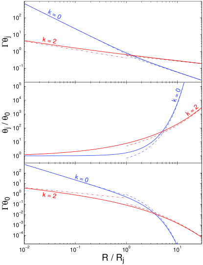
Figure 1: The jet dynamics according to the simple semi-analytic model that is described in the text (solid lines), that is obtained by numerically solving equations (6) and (7) with the initial conditions given by $\theta_{j}(\tilde{R}_{0})=\theta_{0}$ and equation (8). We have used $\beta_{s}=c_{s}/c=3^{-1/2}$, which corresponds the the sound speed of a relativistically hot fluid, and show results for a uniform external medium ($k=0$) and for a stellar wind ($k=2$). Also shown are the analytic approximations for $R_{\rm dec}<R<R_{j}$ (dashed-dotted lines) and for $R_{j}<R<R_{\rm NR}$ (dashed lines, according to equations [10], [13] and [14] with $b=1/4$). For $\Gamma\theta_{j}$ at $R_{j}<R<R_{\rm NR}$ we also show (by the dotted line) the higher order approximation given in footnote 3.

The total swept-up (rest) mass, $M(R)$, is accumulated as

$$\frac{dM}{dR}\approx 2\pi(\theta_{j}R)^{2}\rho_{\rm ext}(R)=2\pi AR^{2-k}\theta_{j}^{2}(R)\ ,$$ (3)

where the factor of $2$ is since a double sided jet is assumed. As long as the jet is relativistic, energy conservation takes the form $E\approx\Gamma^{2}Mc^{2}$, which implies that $Md(\Gamma^{2})=-\Gamma^{2}dM$, and

$$\frac{d\Gamma}{dR}=-\frac{\Gamma}{2M}\frac{dM}{dR}=-\pi AR^{2-k}\theta_{j}^{2}(R)\frac{\Gamma(R)}{M(R)}\ .$$ (4)

One can numerically integrate equations (2), (3), and (4) thus obtaining $\theta_{j}(R)$, $M(R)$, and $\Gamma(R)$. Alternatively, one can use the relation $E\approx\Gamma^{2}Mc^{2}$ (energy conservation) which reduces the number of free variable to two, and solve equations (2) and (4). Changing variables to a dimensionless radius, $\tilde{R}\equiv R/R_{j}$, where

$$R_{j}=\left(\frac{E}{\pi Ac_{s}^{2}}\right)^{1/(3-k)}\ ,$$ (5)

gives

$$\frac{d\theta_{j}}{d\tilde{R}} = \frac{\beta_{s}}{\tilde{R}\,\Gamma(\tilde{R})}\ ,$$ (6)

$$\frac{d\Gamma}{d\tilde{R}} = -\beta_{s}^{-2}\tilde{R}^{2-k}\theta_{j}^{2}(\tilde{R})\Gamma^{3}(\tilde{R})\ .$$ (7)

The initial conditions at some small radius $\tilde{R}_{0}\ll 1$ (just after the deceleration radius) are $\theta_{j}(\tilde{R}_{0})=\theta_{0}$ and

$$\Gamma(\tilde{R}_{0})=\sqrt{\frac{3-k}{2}}\,\frac{\beta_{s}}{\theta_{0}}\,\tilde{R}_{0}^{-(3-k)/2}\ .$$ (8)

Equations (6) and (7) imply,

$$\frac{d(\Gamma\theta_{j})}{d\tilde{R}}\approx\frac{\beta_{s}}{\tilde{R}}-\frac{\tilde{R}^{2-k}}{\beta_{s}^{2}}(\Gamma\theta_{j})^{3}\ .$$ (9)

If one assumes that the first term becomes dominant at $\tilde{R}>1$ then this equation implies $\Gamma\theta_{j}\approx\beta_{s}\ln\tilde{R}$, which in turn implies that the second term would be dominant, rendering the original assumption inconsistent. The same applies if the opposite assumption is made, that the second term is dominant (in this case $\Gamma\theta_{j}\propto\tilde{R}^{(k-3)/2}$ which implies that the first term would be dominant). This implies that the two terms must remain comparable, and therefore

$$\Gamma\theta_{j}\approx\beta_{s}\tilde{R}^{-(3-k)/3}\ .$$ (10)

A similar conclusion can be reach by taking the ratio of equations (6) and (7) which implies that

$$d(\Gamma^{-3})=\beta_{s}^{-3}\tilde{R}^{3-k}d(\theta_{j}^{3})\ .$$ (11)

Substituting equation (10) into equation (6) yields

$$\frac{d\theta_{j}}{d\tilde{R}}\approx\theta_{j}\tilde{R}^{-k/3}\ ,$$ (12)

and

$$\theta_{j} \approx b\theta_{0}\exp\left[\frac{3}{(3-k)}\tilde{R}^{(3-k)/3}\right]\ ,$$ (13)

$$\Gamma \approx \frac{\beta_{s}}{b\theta_{0}}\tilde{R}^{(k-3)/3}\exp\left[-\frac{3}{(3-k)}\tilde{R}^{(3-k)/3}\right]\ ,\quad\quad$$ (14)

where $b\approx 1/4$ is determined numerically.

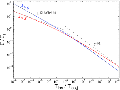
Figure 2: The jet Lorentz factor $\Gamma$ as a function of the observed arrival time of photons emitted along the line of sight $T_{\rm los}\approx\int dR/2c\Gamma^{2}$, for the simple semi-analytic model illustrated in Figure 1 (solid lines). Both $\Gamma$ and $T_{\rm los}$ are normalized to their values at $R_{j}$ extrapolated from $R\ll R_{j}$ ($\Gamma_{j}$ and $T_{\rm los,j}$, respectively). Also shown are the asymptotic scalings at $T_{\rm los}\ll T_{j}$ and $T_{\rm los}\gg T_{j}$.

The results of this simple semi-analytic model are illustrated in Figures 1 and 2. In practice, the dynamical range between the onset of the exponential lateral spreading of the jet (at $R_{j}$) and the non-relativistic transition (at $R_{\rm NR}$) is quite limited. This fact is ignored in these figures, and a wide dynamical range is shown in order to better isolate the characteristics of this intermediate stage ($R_{j}<R<R_{\rm NR}$). The dynamical transition at $R\sim R_{j}$ is much more gradual for a wind environment ($k=2$) compared to a uniform density medium ($k=0$). This leads to a much smoother and more gradual jet break in the afterglow light curve (Kumar & Panaitescu, 2000) which would be hard to detect.

The results derived here are somewhat different than those of Rhoads (1999) who obtained $\Gamma\propto\exp(-\tilde{R})$ and $\theta_{j}\propto\tilde{R}^{-1}\exp(\tilde{R})$ at $R_{j}<R<R_{\rm NR}$ for a uniform external medium ($k=0$), and they are closer (though not identical) to those of Piran (2000). This demonstrates the sensitivity of such semi-analytic models to the exact assumptions that are made. Nevertheless, despite the differences in their details, all of these semi-analytic models for the jet dynamics share a similar main prediction: a very fast lateral expansion (where the jet half opening angle $\theta_{j}$ typically grows exponentially with the radius $R$) after the jet break time. As is discussed in §0.2.2 and §0.2.3, more detailed numerical calculations of the jet dynamics, which better capture the relevant physics, contradict this result and show that the degree of lateral expansion is very modest as long as the jet is relativistic. Therefore, a simple and useful approximation for (semi-) analytic calculations would be that the jet does not expand sideways altogether, retaining its original opening angle and evolving as if it were part of a spherical flow, as long as it is relativistic.

0.2.2 Intermediate Approach: Integrating over the Radial Profile

Figure 3: The dynamics of a jet with an initially (at a lab frame time $t_{0}$) Gaussian profile where the energy per solid angle $\epsilon$ and the Lorentz factor $\Gamma$ are given by $\epsilon,\,\Gamma-1\propto\exp(-\theta^{2}/2\theta_{c}^{2})$, calculated using a scheme where the dynamical equations are simplified by integrating over the radial profile of the shocked fluid (Kumar & Granot, 2003). The parameters used in this calculation are $\theta_{c}=0.035\;$rad, $\Gamma(\theta=0,t_{0})=200$, $\epsilon(\theta=0,t_{0})=10^{53}/4\pi\;{\rm erg/sr}$, $n_{\rm ext}=10\;{\rm cm^{-3}}$. The different panels show the evolution of $\Gamma-1$, $\epsilon$, and the comoving lateral velocity $v^{\prime}_{\theta}/c=\Gamma v_{\theta}/c$. The different curves are for different lab frame times: $v^{\prime}_{\theta}/c$ increases with time, while $\epsilon$ and $\Gamma-1$ decrease with time at the center of the jet and increase with time at the sides of the jet behind what appears as a shock in the lateral direction which propagates to larger angles $\theta$.

The over-simplified treatment of the jet dynamics in simple semi-analytic models, and the fact that different such models obtained different results, put into question the validity of those results and motivated more careful studies of the jet dynamics. A proper treatment of this problem requires a full hydrodynamic simulation (in at least 2D) and is discussed in the next subsection. However, since such simulations are very challenging numerically, an intermediate approach between simple semi-analytic models and full hydrodynamic simulations can be useful. This was attempted by Kumar & Granot (2003) and is briefly described here. Under the assumption of axial symmetry, the dynamical equations are reduced to two spatial dimensions. The dynamical equations can be reduced to a set of one dimensional (1D) partial differential equations (PDEs), and thus greatly reducing the computational difficulty involved in solving these equations, by integrating over the radial profile of the shocked fluid in the jet. The motivation for this, apart from making the calculations much easier, is that most of the shocked fluid is concentrated within a very thin layer behind the shock, of width $\Delta\sim R/10\Gamma^{2}$ in the lab frame (i.e. the frame of the unperturbed external medium). This suggests that integrating over the radial profile might not introduce a very large error in the calculation of the jet dynamics.

Figure 4: The dynamics of a “structured” jet where initially $\Gamma-1=200/(1+\theta^{2}/\theta_{c}^{2})$ and $\epsilon=\epsilon_{0}/(1-\theta^{2}/\theta_{c}^{2})$ with $\epsilon_{0}=10^{53}/4\pi\;{\rm erg/sr}$, $\theta_{c}=0.02\;$rad, and $n_{\rm ext}=10\;{\rm cm^{-3}}$. The format is similar to Figure 3. Again $v^{\prime}_{\theta}/c$ increases with time while $\Gamma-1$ decreases with time. For a structured jet, as opposed to an initially Gaussian jet, a shock does not develop in the lateral direction and $\epsilon(\theta)$ remains almost unchanged as long as the jet is relativistic.

The results of this method are shown in Figure 3 for a jet with an initial Gaussian profile in $\Gamma-1$ and in the energy per solid angles $\epsilon=dE/d\Omega$. Such a jet can be thought of as a smoother and therefore more realistic version of a uniform jet, since it has a roughly uniform core and relatively sharp (but still smooth) wings. A shock appears to develop in the lateral direction, because of the very steep initial angular profile in the wings of the Gaussian. Nevertheless, the lateral expansion remains modest as long as the jet is relativistic. This can be seen both from the small (compared to $c$) lateral velocity in the comoving frame, and from the fact that $\epsilon(\theta)$ does not change very much compared to its initial distribution. The modest degree of lateral spreading is in stark contrast with the results of semi-analytic models.

Figure 4 shows the resulting dynamics for a “structured” jet (which is discussed in §0.3) where $\Gamma$ and $\epsilon$ are initially power laws with the angle $\theta$ from the jet symmetry axis, outside of some narrow core. Again, there is very little lateral expansion (i.e. the comoving lateral velocity remains $\ll c$ and $\epsilon(\theta)$ hardly deviates from its initial profile) as long as the jet core is relativistic.

0.2.3 Hydrodynamic Simulations

The most reliable method for calculating the jet dynamics is using hydrodynamic simulations. This is a formidable numerical task for the following reasons. First, it requires a hydrodynamic code with special relativity that is accurate over a large range in the four velocity $u=\Gamma\beta$, from $u\approx\Gamma\gg 1$ to $u\approx\beta\ll 1$. Second, the shocked fluid in the jet is concentrated in a very thin layer behind the shock, of width $\Delta\sim R/10\Gamma^{2}$ in the lab frame, which is extremely narrow at early times when $\Gamma\gg 1$, and therefore very hard to resolve properly.

More specifically, from considerations of causality, significant lateral expansion could in principal occur when $\Gamma$ becomes comparable to $\theta_{0}^{-1}$, so that ideally one would want to start with an initial Lorentz factor $\Gamma_{0}\gg\theta_{0}^{-1}$, and in practice we need at least $\Gamma_{0}\theta_{0}\gtrsim\;{\rm a\ few}$. Observed jet break times suggest $0.05\lesssim\theta_{0}\lesssim 0.2$ and therefore require $\Gamma_{0}\gtrsim 20-100$. If $100N_{2}$ cells are needed in order to resolve the shell of width $\Delta\sim R/10\Gamma^{2}$ then the minimal cell size in the initial time step (denoted by the subscript ‘0’) needs to be of the order of $\delta\sim 10^{-6}N_{2}^{-1}(\Gamma_{0}/30)^{-2}R_{0}\sim 10^{-6}N_{2}^{-1}(\Gamma_{0}\theta_{0}/3)^{-2}(\theta_{0}/0.1)^{2}R_{0}$. The minimal number of cells required to resolve the initial shell is $N_{\rm min}\sim\theta_{0}R_{0}\Delta_{0}\delta^{-2}\sim 10^{7}N_{2}^{2}(\Gamma_{0}\theta_{0}/3)^{2}(\theta_{0}/0.1)^{-1}$. The total number of cells in each time step can be $N_{\rm tot}\sim N_{\rm min}$ if the code uses adaptive mesh refinement (AMR). Otherwise, for a fixed cell size, $N_{\rm tot}/N_{\rm min}\gtrsim R_{0}/\Delta_{0}\sim 10^{4}(\Gamma_{0}\theta_{0}/3)^{2}(\theta_{0}/0.1)^{-2}$.

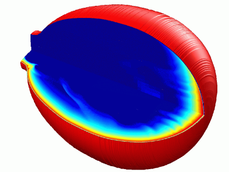
Figure 5: A 3D view of a relativistic impulsive jet at the last time step of the simulation (Granot et al., 2001). The outer surface represents the shock front while the two inner faces show the proper number density (lower face) and proper synchrotron emissivity (upper face) in a logarithmic color scale.

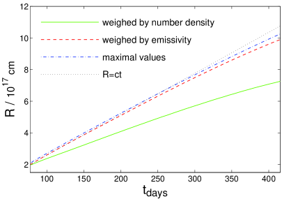
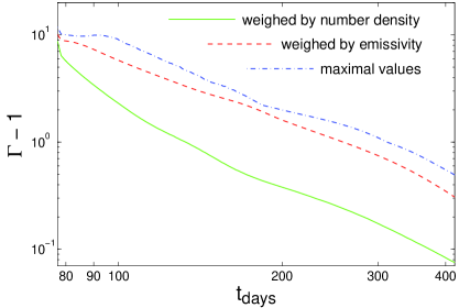
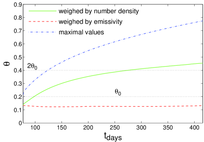
Figure 6: The jet radius (upper panel), Lorentz factor minus one (middle panel), and angle $\theta$ from the jet symmetry axis (lower panel), as a function of the lab frame time $t_{\rm lab}\approx R/c$ (in days), from a hydrodynamic simulation (Granot et al., 2001).

Because of the numerical difficulty involved, very few attempts have been made so far (Granot et al., 2001; Cannizzo et al., 2004). In the following I shall concentrate on the results of Granot et al. (2001). The initial conditions were a cone of half-opening angle $\theta_{0}=0.2\;$rad, taken out of the spherical Blandford & McKee (1976) self-similar solution with an (isotropic equivalent) energy of $E_{\rm k,iso}=10^{52}\;$erg and a uniform external density of $n_{\rm ext}=1\;{\rm cm^{-3}}$. The initial Lorentz factor of the fluid just behind the shock was $\Gamma_{0}\approx 16.8$ corresponding to $\Gamma_{0}\theta_{0}\approx 3.4$.

The results of the simulation are illustrated in Figures 5 and 6. While the number density does not change significantly between the front and the sides of the jet, the emissivity is large only at the front of the jet, within its initial half-opening angle ($\theta<\theta_{0}$), and drops sharply at $\theta>\theta_{0}$. This causes the emissivity weighted values of the Lorentz factor and radius to be close to their maximal values (which are also obtained at the front of the jet). While the sides of the jet contribute a small fraction of the total emissivity, their emission can dominate the observed flux for lines of sight outside the initial half-opening angle of the jet, as discussed in §0.3.5. The overall egg-shaped structure of the shock front is very different from the quasi-spherical structure assumed in 1D semi-analytic models. Moreover, the degree of lateral expansion is very modest as long as the head of the jet is relativistic, in contradiction with the very rapid lateral expansion predicted by semi-analytic models.

0.2.4 The Afterglow Emission

The dominant emission mechanism during the afterglow stage is believed to be synchrotron emission. This is supported by the detection of linear polarization at the level of $\sim 1\%-3\%$ in several optical or NIR afterglows (see §0.3.3), and by the shape of the broad band spectrum, which consists of several power-law segments that smoothly join at some typical break frequencies. Synchrotron self-Compton (SSC; the inverse-Compton scattering of the synchrotron photons by the same population of relativistic electrons that emits the synchrotron photons) can sometimes dominate the afterglow flux in the X-rays (Sari & Esin, 2001; Harrison et al., 2001).

Figure 7: The afterglow synchrotron spectrum, calculated for the Blandford & McKee (1976) spherical self-similar solution, under standard assumptions, using the accurate form of the synchrotron spectral emissivity and integration over the emission from the whole volume of shocked material behind the forward (afterglow) shock (for details see Granot & Sari, 2002). The different panels show the five possible broad band spectra of the afterglow synchrotron emission, each corresponding to a different ordering of the spectral break frequencies. Each spectrum consists of several power law segments (PLSs; each shown with a different color and labeled by a different letter A–H) that smoothly join at the break frequencies (numbered 1–11). The broken power law spectrum, which consists of the asymptotic PLSs that abruptly join at the break frequencies (and is widely used in the literature), is shown for comparison. Most PLSs appear in more than one of the five different broad band spectra. Indicated next to the arrows are the temporal scaling of the break frequencies and the flux density at the different PLSs, for a uniform (ISM) and stellar wind (WIND) external density profile.

It is usually assumed that the electrons are (practically instantaneously) shock-accelerated into a power law distribution of energies, $dN/d\gamma_{e}\propto\gamma_{e}^{-p}$ for $\gamma_{e}>\gamma_{m}$, and thereafter cool both adiabatically and due to radiative losses. Furthermore, it is assumed that practically all of the electrons take part in this acceleration process and form such a non-thermal (power-law) distribution, leaving no thermal component (which is not at all clear or justified; e.g. Eichler & Waxman, 2005). The relativistic electrons are assumed to hold a fraction $\epsilon_{e}$ of the internal energy immediately behind the shock, while the magnetic field is assumed to hold a fraction $\epsilon_{B}$ of the internal energy everywhere in the shocked region. This is a convenient parameterization of our ignorance regarding the micro-physics of relativistic collisionless shocks, which are still not sufficiently well understood from first principals.

The spectral emissivity in the co-moving frame of the emitting shocked material is typically approximated as a broken power-law (in some cases the more accurate functional form of the synchrotron emission is used, e.g. Wijers & Galama, 1999; Granot & Sari, 2002). Most calculations of the light curve assume emission from an infinitely thin shell, which represents the shock front (some integrate over the volume of the shocked fluid taking into account the appropriate radial profile of the flow, e.g. Granot & Sari, 2002, see Figure 7). One also needs to account for the different arrival times of photons to the observer from emission at different lab frame times and locations relative to the line of sight, as well as the relevant Lorentz transformations of the emission into the observer frame. SSC is included in some (not all) works, although it can also effect the synchrotron emission through the enhanced radiative cooling of the electrons.

0.2.5 The afterglow Image

The apparent surface brightness distribution and size evolution of the afterglow image on the plane of the sky can potentially provide very useful information about the structure and dynamics of GRB jets, as well as about the radial dependence of the external density. Furthermore, polarimetry (or even spectral polarimetry) of a resolved afterglow image could provide valuable information on the magnetic field structure behind collisionless relativistic shocks, which is not well understood theoretically. However, most GRBs are at cosmological distances ($z\gtrsim 1$) and the angular size of their afterglow image is of the order of a micro-arcsecond ($\mu$as) after a day or so, making it extremely difficult to resolve the image.

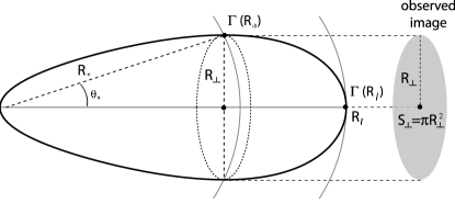
Figure 8: Schematic illustration of the equal arrival time surface (thick black line), namely, the surface from where the photons emitted at the shock front arrive at the same time to the observer (on the far right-hand side). The maximal lateral extent of the observed image, $R_{\perp}$, is located at an angle , where the shock radius and Lorentz factor are $R_{*}$ and $\Gamma_{*}=\Gamma_{\rm sh}(R_{*})$, respectively. The area of the image on the plane of the sky is $S_{\perp}=\pi R_{\perp}^{2}$. The shock Lorentz factor, $\Gamma_{\rm sh}$, varies with radius $R$ and angle $\theta$ from the line of sight along the equal arrival time surface. The maximal radius $R_{l}$ on the equal arrival time surface is located along the line of sight. If, as expected, $\Gamma_{\rm sh}$ decreases with $R$, then $\Gamma_{l}=\Gamma_{\rm sh}(R_{l})$ is the minimal shock Lorentz factor on the equal arrival time surface. (from Granot, Ramirez-Ruiz & Loeb, 2005).

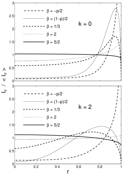
Figure 9: The afterglow images for different power law segments of the spectrum, for a uniform ($k=0$) and wind ($k=2$) external density profile (from Granot & Loeb, 2001, calculated for the Blandford & McKee 1976 spherical self similar solution, using the formalism of Granot & Sari 2002). Shown is the surface brightness, normalized by its average value, as a function of the normalized distance from the center of the image, $r=R\sin\theta/R_{\perp}$ (where $r=0$ at the center and $r=1$ at the outer edge). The image profile changes considerably between different power-law segments of the afterglow spectrum, $F_{\nu}\propto\nu^{\beta}$. There is also a strong dependence on the density profile of the external medium, $\rho_{\rm ext}\propto R^{-k}$.

During the self-similar spherical evolution stage (before the jet break time, for a jet), the afterglow image has circular symmetry around the line of sight (where the surface brightness depends only on the distance from the center of the image), and is confined within a circle on the sky with a radius

$$\frac{R_{\perp}}{10^{16}\;{\rm cm}}=\left\{\matrix{3.91\left(\frac{E_{52}}{n_{0}}\right)^{1/8}\left(\frac{t_{\rm days}}{1+z}\right)^{5/8}&\ \ (k=0)\cr&\cr 2.39\left(\frac{E_{52}}{A_{*}}\right)^{1/4}\left(\frac{t_{\rm days}}{1+z}\right)^{3/4}&\ \ (k=2)}\right.\ .$$ (15)

(see Figure 8) where $E_{52}$ is the isotropic equivalent afterglow kinetic energy in units of $10^{52}\;$erg, $t_{\rm days}$ is the observed time in days, and the external density is assumed to be a power law with the distance $R$ from the central source, $\rho_{\rm ext}=n_{\rm ext}m_{p}=AR^{-k}$, where $n_{0}=n_{\rm ext}/(1\;{\rm cm^{-3}})$ for a uniform external density ($k=0$), and $A_{*}=A/(5\times 10^{11}\;{\rm g\;cm^{-1}})$ for a wind-like external density profile ($k=2$) as might be expected for a massive star progenitor. This corresponds to an angular radius of

$$\frac{R_{\perp}}{d_{A}}=\left\{\matrix{\frac{1.61\;\mu{\rm as}}{d_{A,27.7}}\left(\frac{E_{52}}{n_{0}}\right)^{1/8}\left(\frac{t_{\rm days}}{1+z}\right)^{5/8}&\ \ (k=0)\cr&\cr\frac{0.98\;\mu{\rm as}}{d_{A,27.7}}\left(\frac{E_{52}}{A_{*}}\right)^{1/4}\left(\frac{t_{\rm days}}{1+z}\right)^{3/4}&\ \ (k=2)}\right.\ .$$ (16)

where $d_{A}(z)$ is the angular distance to the source, and $d_{A,27.7}$ is $d_{A}$ in units of $10^{27.7}\;{\rm cm}\approx 5\times 10^{27}\;$cm. 

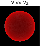
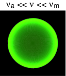
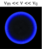
Figure 10: An illustration of the expected afterglow image on the plain of the sky, for three different power law segments of the spectrum (from Granot, Piran & Sari, 1999a, b), assuming a uniform external density and the Blandford & McKee (1976) self-similar solution. The image is more limb brightened at power law segments that correspond to higher frequencies.

More generally, the afterglow image size during the self-similar spherical stage scales with the observed time as $R_{\perp}\propto t^{(5-k)/2(4-k)}$. The image size grows super-luminally with an apparent expansion velocity of $\Gamma_{\rm sh}(R_{*})c$. The expected afterglow images in this self-similar regime are shown in Figures 9 and 10. The normalized surface brightness profile within the afterglow image is independent of time due to the self-similar dynamics, and changes only between the different power law segments of the synchrotron spectrum, and for different external density profiles. The image becomes increasingly limb-brightened at higher frequencies, and for smaller values of $k$.

Below the self-absorption frequency the specific intensity (surface brightness) represents the Rayleigh-Jeans portion of a black-body spectrum with the blue-shifted effective temperature of the electrons at the corresponding radius along the front side of the equal arrival time surface of photons to the observer ($R_{*}\leq R\leq R_{l}$ in Figure 8). Above the cooling break frequency the emission originates from a very thin layer behind the shock front where the electrons whose typical synchrotron frequency is close to the observed frequency have not yet had enough time to significantly cool due to radiative losses. This results in a divergence of the surface brightness at the outer edge of the image (Sari, 1998; Granot & Loeb, 2001).

After the jet break time the afterglow image is no longer symmetric around the line of sight to the central source for a general viewing angle (which is not exactly along the jet symmetry axis), and its details depend on the the hydrodynamic evolution of the jet (so that in principal it could be used in order to constrain the jet dynamics). Therefore, a realistic calculation of the afterglow image during the more complicated post-jet break stage requires the use of hydrodynamic simulation, and still remains to be done.

The afterglow image may be indirectly resolved through gravitational lensing by a star in an intervening galaxy (along, or close to, our line of sight to the source). This is since the angular size of the Einstein radius (i.e. the region of large magnification around the lensing star) for a typical star at a cosmological distance is $\sim 1\;\mu$as (hence the name micro-lensing), and therefore comparable to the afterglow image size after a day or so. Since the afterglow image size grows very rapidly with time, different parts of the image sample the regions of large magnification (close to the point of infinite magnification just behind the lensing star) with time, and therefore the overall magnification of the afterglow flux as a function of time probes the surface brightness profile of the afterglow image. This results in a bump in the afterglow light curve which peaks when the limb-brightened outer part of the image sweeps past the lensing star, where the peak of the bump is sharper the more limb-brightened the afterglow image (Granot & Loeb, 2001). It has been suggested that an achromatic bump in the afterglow light curve of GRB 000301C after $\sim 4\;$days might have been due to micro-lensing (Garnavich, Loeb & Stanek, 2000). If this interpretation is true, then the shape of the bump in the afterglow light curve requires a limb-brightened afterglow image, in agreement with theoretical expectations (Gaudi, Granot & Loeb, 2001).

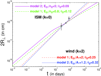
Figure 11: Tentative fits to the constraints on the image size (or diameter $2R_{\perp}$) of the radio afterglow of GRB 030329 at different epochs, for different external density profiles and different assumptions on the lateral spreading of the jet. The physical parameters and external density profile for each model are indicated (the viewing angle is along the jet symmetry axis). Model 1 features relativistic sideways expansion in the co-moving rest frame of the jet material, while model 2 has no lateral spreading (from Granot, Ramirez-Ruiz & Loeb, 2005).

The size of the afterglow image at a single epoch can be estimated from the quenching of diffractive scintillations in the radio afterglow (Goodman, 1997; Frail et al., 1997; Taylor et al., 1997; Waxman, Kulkarni & Frail, 1998). The flux below the self-absorption frequency can also be used to constrain the size of the emitting region (e.g., Katz & Piran, 1997; Granot, Ramirez-Ruiz & Loeb, 2005). A more direct measurement of the image size, as well as its temporal evolution, may be obtained through very large base-line interferometry in the radio (i.e. with the VLBA). This was possible for only for one radio afterglow so far (GRB 030329; Taylor et al., 2004, 2005), since it requires a relatively nearby event ($z\lesssim 0.2$) with a bright radio afterglow. Nevertheless, it already provides interesting constraints (Oren, Nakar & Piran, 2004; Granot, Ramirez-Ruiz & Loeb, 2005, see Figure 11), and better observations in the future may help pin down the jet structure and dynamics, as well as the external density profile.

0.2.6 What causes the Jet Break?

The jet break in the afterglow light curve has been argued to be the combination of (i) the edge of the jet becoming visible, and (ii) fast lateral spreading. Both effects are expected to take place around the same time, when the Lorentz factor, $\Gamma$, of the jet drops below the inverse of its initial half-opening angle, $\theta_{0}$. This can be understood as follows.

When $\Gamma$ drops below $\theta_{0}^{-1}$ the edge of the jet becomes visible, since relativistic beaming limits the region from which a significant fraction of the emitted radiation reaches the observer to within an angle of $\sim\Gamma^{-1}$ around the line of sight ($\theta\lesssim\Gamma^{-1}$). Once the edge of the jet becomes visible, then if there is no significant lateral spreading, only a small fraction $(\Gamma\theta_{j})^{2}<1$ of the visible region is occupied by the jet, and therefore there would be “missing” contributions to the observed flux compared to a spherical flow. This would cause a steepening in the light curve, i.e. a jet break, where the temporal decay index asymptotically increases by $\Delta\alpha=(3-k)/(4-k)$.

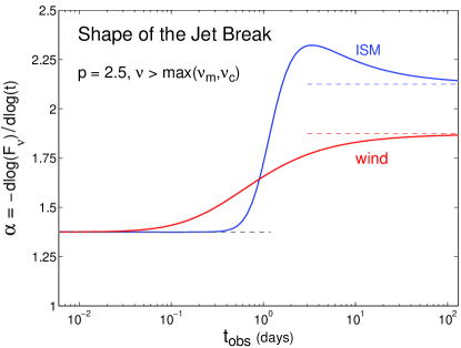
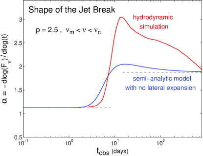
Figure 12: The temporal decay index $\alpha$ as a function of the observed time (in days) across the jet break in the light curve, for $p=2.5$. Upper panel: results in the spectral range $\nu>\max(\nu_{m},\nu_{c})$ using a semi-analytic model with no lateral spreading (Granot, 2005), for a uniform ($k=0$, $n_{\rm ext}=1\;{\rm cm^{-3}}$) and wind ($k=2$, $A_{*}=1$) external density profile, with $\theta_{0}=0.1$ and $E_{\rm k,iso}=2\times 10^{53}\;$erg. Lower panel: results for the spectral range $\nu_{m}<\nu<\nu_{c}$, for $\theta_{0}=0.2$ and a uniform density ($k=0$, $n_{\rm ext}=1\;{\rm cm^{-3}}$, $E_{\rm k,iso}=10^{52}\;$erg); compares the result of a semi-analytic model (Granot, 2005) to those of a hydrodynamic simulation (Granot et al., 2001). In both panels the dashed lines show the asymptotic values of $\alpha$ before and after the jet break, for a uniform jet with no lateral spreading, for which $\Delta\alpha=(3-k)/(4-k)$.

When $\Gamma$ drops below $\theta_{0}^{-1}$, the center of the jet comes into causal contact with its edge, and the jet can in principal start to expand sideways significantly. It has been argued that at this stage it would indeed start to expand sideways rapidly, at close to the speed of light in its own rest frame. In this case, during the rapid lateral expansion phase the jet opening angle grows as $\theta_{j}\sim\Gamma^{-1}$ and exponentially with radius (see §0.2.1). This causes the energy per solid angle, $\epsilon$, in the jet to drop with observed time, and the Lorentz factor to decrease faster as a function of the observed time, which result a steepening in the afterglow light curve compared to a spherical flow (where $\epsilon$ remains constant and $\Gamma$ decreases more slowly with the observed time). However, in this case a good part of the visible region remains occupied by the jet (since $\Gamma\theta_{j}$ remains $\sim 1$), so that the first cause for the jet break (the edge of the jet becoming visible, and the “missing” contributions from outside the edge of the jet) is no longer important. Therefore, for fast lateral spreading, the jet break is caused predominantly since the energy per solid angle $\epsilon$ decreases with time, and the Lorentz factor decreases with observed time faster than for a spherical flow.

It is important to keep in mind, however, that numerical studies show that the lateral spreading of the jet is very modest as long as it is relativistic (see §0.2.2 and §0.2.3). This implies that lateral spreading cannot play an important role in the jet break, and the predominant cause of the jet break is the “missing” contribution from outside of the jet, once its edge becomes visible.

A potential problem with this picture is that if the jet half-opening angle remains roughly constant, $\theta_{j}\approx\theta_{0}$, the asymptotic change in the temporal decay index is only $\Delta\alpha=3/4$ for a uniform external medium ($k=0$) or even smaller for a wind ($\Delta\alpha=1/2$ for $k=2$), while the values inferred from observations are in most cases larger (see Figure 3 of Zeh, Klose & Kann, 2006). This apparent discrepancy may be reconciled as follows. While the asymptotic steepening is indeed $\Delta\alpha=(3-k)/(4-k)$ when lateral expansion is negligible, the value of the temporal decay index $\alpha$ (where $F_{\nu}\propto t^{-\alpha}$) initially overshoots its asymptotic value. Since the temporal baseline that is used in order to measure the post-jet break temporal decay index $\alpha_{2}$ is typically no more than a factor of several in time after the jet break time, $t_{\rm jet}$, the value of $\alpha$ during this time is larger than its asymptotic value $\alpha_{2}$. This causes the value of $\Delta\alpha$ that is inferred from observations to be larger than its asymptotic value.

The overshoot in the value of $\alpha$ just after the jet break time can nicely be seen in Figure 12, and is much more pronounced in the light curves calculated using the jet dynamics from a hydrodynamic simulation, compared to the results of a simple semi-analytic model. The cause of this overshoot is that the afterglow image is limb-brightened (see Figure 9) and therefore the outer edges of the image which are the brightest are the first region whose contribution to the observed flux is “missed” as the edge of the jet becomes visible. The overshoot is larger the more limb-brightened the afterglow image (e.g., for $\nu>\max(\nu_{m},\nu_{c})$ in the upper panel of Figure 12 compared to $\nu_{m}<\nu<\nu_{c}$ in the lower panel of Figure 12). For a wind density ($k=2$) the limb-brightening is smaller compared to a uniform density ($k=0$), at the same power law segment of the spectrum (see Figure 9), and the Lorentz factor $\Gamma$ decreases more slowly with the observed time. Because of this no overshoot is seen in the semi-analytic model shown in the upper panel of Figure 12 for a wind density profile ($k=2$), and the jet break is smoother and extends over a larger factor in time. The asymptotic post-jet break value of the temporal decay index ($\alpha_{2}$) is approached only when the visible part of the afterglow image covers the relatively uniform central part, and not its brighter outer edge.

The jet break in light curves calculated from hydrodynamic simulations is sharper than in semi-analytic models (where the emission is taken to be from a 2D surface – usually a section of a sphere within a cone). In semi-analytic models the jet break is sharpest with no lateral expansion, and becomes more gradual the faster the assumed lateral expansion. For example, in the lower panel of Figure 12, where the viewing angle is along the jet axis and the external density is uniform, most of the change in the temporal decay index $\alpha$ occurs over a factor of $\sim 2$ in time for the numerical simulation, and over a factor of $\sim 3$ in time for the semi-analytic model (which assumes no lateral expansion; the jet break would be more gradual with lateral expansion). For both types of models, the jet break is more gradual and occurs at a somewhat later time for viewing angles further away from the jet symmetry axis but still within its initial opening angle, although this effect is somewhat more pronounced in semi-analytic models (Granot et al., 2001; Rossi et al., 2004).

0.3 The Jet Structure

Since the initial discovery of GRB afterglows in the X-ray (Costa et al., 1997), optical (van Paradijs et al., 1997), and radio (Frail et al., 1997), many afterglows have been detected and the quality of individual afterglow light curves has improved dramatically (e.g., Lipkin et al., 2004). Despite all the observational and theoretical progress, the structure of GRB jets remains largely an open question. This question is of great importance and interest, since it is related to issues that are fundamental for our understanding of GRBs, such as their event rate, total energy, and the requirements from the compact source that accelerates and collimates these jets.

In §0.3.1 a brief overview is given of the main jet structures that have been discussed in the literature and the motivation for them. This is followed by a discussion of the different methods that have been applied for constraining the jet structure from observations, which include statistical studies (§0.3.2), as well as the evolution of the linear polarization of the afterglow emission (§0.3.3), and the shape of the afterglow light curves (§0.3.4). The afterglow light curves from viewing angles outside the initial jet aperture are discussed in §0.3.5 along with possible implications for X-ray flashes and for the jet structure, while §0.3.6 briefly mentions the search for orphan afterglows. Some implications of recent Swift observations are discussed in §0.3.7.

0.3.1 Existing Models for the Jet Structure

The leading models for the jet structure are (i) the uniform jet (UJ) model (Rhoads, 1997, 1999; Panaitescu & Mészáros, 1999; Sari, Piran & Halpern, 1999; Kumar & Panaitescu, 2000; Moderski, Sikora & Bulik, 2000; Granot et al., 2001, 2002), where the energy per solid angle, $\epsilon$, and the initial Lorentz factor, $\Gamma_{0}$, are uniform within some finite half-opening angle, $\theta_{j}$, and sharply drop outside of $\theta_{j}$; and (ii) the universal structured jet (USJ) model (Lipunov, Postnov & Prokhorov, 2001; Rossi et al., 2002; Zhang & Mészáros, 2002), where $\epsilon$ and $\Gamma_{0}$ vary smoothly with the angle $\theta$ from the jet symmetry axis. In the UJ model the different values of the jet break time, $t_{j}$ , in the afterglow light curve arise mainly due to different $\theta_{j}$ (and to a lesser extent due to different ambient densities). In the USJ model, all GRB jets are intrinsically identical, and the different values of $t_{j}$ arise mainly due to different viewing angles, $\theta_{\rm obs}$, from the jet axis.

The observed correlation, $t_{j}\propto E_{\rm\gamma,iso}^{-1}$ (Frail et al., 2001; Bloom, Frail & Kulkarni, 2003), implies a roughly constant true energy, $E$, between different GRB jets in the UJ model, and $\epsilon\propto\theta^{-2}$ outside of some core angle, $\theta_{c}$, in the USJ model (Rossi et al., 2002; Zhang & Mészáros, 2002). This is assuming a constant efficiency, $\epsilon_{\gamma}$, for producing the observed prompt gamma-ray (or X-ray) emission. If the efficiency depends on $\theta$ in the USJ model, for example, then different power laws of $\epsilon$ with $\theta$ are possible (Guetta, Granot & Begelman, 2005), such as a core with wings where $\epsilon\propto\theta^{-3}$, as is obtained in simulations of the collapsar model (Zhang, Woosley & MacFadyen, 2003; Zhang, Woosley & Heger, 2004).

The jet structure was initially envisioned to be uniform since this is the simplest jet structure, and arguably also the most natural. Furthermore, it also predicted a jet break in the afterglow light curve (Rhoads, 1997, 1999; Sari, Piran & Halpern, 1999), which was soon thereafter confirmed observationally (Fruchter et al., 1999; Kulkarni et al., 1999a; Stanek et al., 1999). The original motivation for the USJ model was the conceptual simplicity of a universal intrinsic structure for all GRB jets, where the observed differences (namely in the jet break times) arise due to different viewing angles (instead of being attributed to an intrinsic difference - in the jet half-opening angle - as in the UJ model). Its exact structure was motivated by the requirement to reproduce the observed afterglow light curves and correlations with the prompt GRB emission. It had later been suggested on theoretical grounds that a jet structure with a narrow core and wings where $\epsilon\propto\theta^{-2}$ is expected in highly magnetized Poynting flux dominated jets (Lyutikov & Blandford, 2002, 2003) as well as in low magnetization hydrodynamic jets in the context of the collapsar model (Lazzati & Begelman 2005; see, however, Morsony, Lazzati & Begelman 2006).

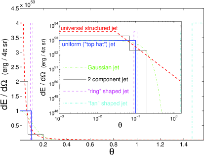
Figure 13: An illustration of various jet structures that have been discussed in the literature, in terms of the distribution of their energy per solid angle, $\epsilon=dE/d\Omega$, with the angle $\theta$ from the jet symmetry axis, both in semi-logarithmic scale (main figure) and in log-log scale (big inset). Both the normalization of $dE/d\Omega$ and the typical angular scale may vary in most models, and their values shown here were chosen to be more or less “typical”. (from Granot, 2005).

Other jet structures have also been proposed in the literature. Figure 13 illustrates different jet structures that have been discussed in the literature in terms of their distribution of $\epsilon(\theta)$. A jet with a Gaussian angular profile (Zhang & Mészáros, 2002; Kumar & Granot, 2003) may be thought of as a more realistic version of a uniform jet, where the edges are smooth rather than sharp. A Gaussian $\epsilon(\theta)\propto\exp(-\theta^{2}/2\theta_{c}^{2})$ is approximately intermediate between the UJ and USJ models, but it is closer to the UJ model than to the USJ model with $\epsilon\propto\theta^{-2}$ in the sense that for a Gaussian $\epsilon(\theta)$ the energy in the wings of the jet is much smaller than in its core, whereas for a USJ with $\epsilon\propto\theta^{-2}$ wings there is equal energy per decade in the wings, and therefore the wings contain more energy than the core (by about an order of magnitude).

Another jet structure that received some attention recently is a two-component jet model (Pedersen et al., 1998; Frail et al., 2000; Berger et al., 2003b; Huang et al., 2004; Peng, Königl & Granot, 2005; Wu et al., 2005) with a narrow uniform jet of initial Lorentz factor $\Gamma_{0}\gtrsim 100$ surrounded by a wider uniform jet with $\Gamma_{0}\sim 10-30$. Theoretical motivation for such a jet structure has been found both in the context of the cocoon in the collapsar model (Ramirez-Ruiz, Celotti & Rees, 2002) and in the context of a hydromagnetically driven neutron-rich jet (Vlahakis, Peng & Königl, 2003). This model has been invoked in order to account for sharp bumps (i.e., fast rebrightening episodes) in the afterglow light curves of GRB 030329 (Berger et al., 2003b) and XRF 030723 (Huang et al., 2004). A different motivation for proposing this jet structure is in order to account for the energetics of GRBs and X-ray flashes and reduce the high efficiency requirements from the prompt gamma-ray emission (Peng, Königl & Granot, 2005).

More “exotic” jet structures have also been considered. One example is a jet with a cross section in the shape of a “ring,” sometimes referred to as a “hollow cone” (Levinson & Eichler, 1993, 2000; Eichler & Levinson, 2003, 2004; Lazzati & Begelman, 2005), which is uniform within $\theta_{c}<\theta<\theta_{c}+\Delta\theta$ where $\Delta\theta\ll\theta_{c}$. Another example is a “fan”- or “sheet”-shaped jet (Thompson, 2005) where a magnetocentrifugally launched wind from the proto-neutron star, formed during the supernova explosion in the massive star progenitor, becomes relativistic as the density in its immediate vicinity drops and is envisioned to form a thin sheath of relativistic outflow that is somehow able to penetrate through the progenitor star along the rotational equator, forming a relativistic outflow within $\Delta\theta\ll 1$ around $\theta=\pi/2$ (or $\theta_{c}=\pi/2-\Delta\theta/2$).

0.3.2 Statistical Studies

One approach for constraining the jet structure is through statistical studies of the prompt emission. In particular, a convenient observable is the $\log N-\log S$ distribution, where $N$ is the number of GRBs observed above a limiting peak photon flux $S$ (Firmani et al., 2004; Guetta, Piran & Waxman, 2005; Guetta, Granot & Begelman, 2005; Xu et al., 2005). In this type of study one needs to assume both the intrinsic GRB event rate (which is usually assumed to follow the star formation rate), and the luminosity function which depends on the jet structure through the isotropic equivalent luminosity $L(\theta)$ as a function of the angle $\theta$ from the jet symmetry axis. The latter depends in turn on the angular distribution of the energy per solid angle in the jet $\epsilon(\theta)$ and the gamma-ray efficiency $\epsilon_{\gamma}(\theta)$, whose product (times $4\pi$) provides the isotropic equivalent energy output in gamma-rays, $E_{\rm\gamma,iso}(\theta)$, and the assumed distribution of the peak isotropic equivalent luminosity for a given $E_{\rm\gamma,iso}$.

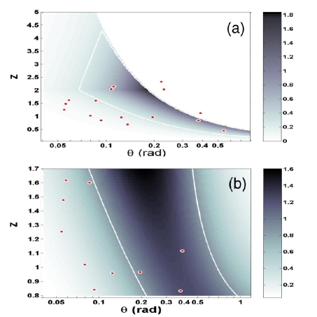
Figure 14: The probability distribution, $dN/dzd\ln\theta$, of the observed GRB rate as a function of redshift $z$ and viewing angle $\theta$, as predicted by the USJ model (from Nakar, Granot & Guetta, 2004). The white contour lines confine the minimal area that contains $1\;\sigma$ of the total probability. The circles denote the 16 GRBs with known $z$ and $\theta$ from the sample of Bloom, Frail & Kulkarni (2003). (a) The model parameters are similar to those of Perna, Sari & Frail (2003). This figure is the 2D realization of their Figure 1. (b) Here a limited range in redshift is used, $0.8<z<1.7$ (containing 10 out of the 16 data points), in order to minimize redshift selection effects and reduce the sensitivity of the results to the unknown GRB rate. Measurement errors of 20% in $\ln\theta$ ($\sigma_{\ln\theta}=0.2$) were included and a log-normal distribution in the effective duration that they deduced from observations.

For the USJ model $\epsilon(\theta)$ and $\epsilon_{\gamma}(\theta)$ are assumed to be power laws in $\theta$ and one needs to specify their power law indexes, as well as the jet core angle $\theta_{c}$ and outer edge $\theta_{\rm max}$ (Guetta, Granot & Begelman, 2005). For the UJ model one needs to specify the distribution of jet half-opening angles $\theta_{0}$, which can be taken to be a power law distribution in the range $\theta_{\rm min}<\theta_{0}<\theta_{\rm max}$. These simple forms of the USJ and UJ models are degenerate, since they both produce a power law luminosity function (Guetta, Granot & Begelman, 2005), which provides an adequate fit to the data. The total rate of energy release in gamma-rays must be the same in both models (and match the observed rate), where in the USJ model it is released in fewer more energetic events (by a factor of $\sim 10$; see equation 14 of Guetta, Granot & Begelman, 2005), while in the UJ model it is released in more numerous less energetic events (i.e. the UJ model predicts a larger intrinsic event rate).

Another statistical approach for constraining the jet structure is through the distribution of the observed number of GRBs $N$ as a function of the angle $\theta$ that is inferred from the observed jet break times in the afterglow light curves, where $\theta$ corresponds to the jet half-opening angle $\theta_{0}$ in the UJ model and to the viewing angle $\theta_{\rm obs}$ in the USJ model. The observed $dN/d\theta$ distribution agrees reasonably well with the predictions of the USJ model (Perna, Sari & Frail, 2003), which had been argued to support the USJ model (since in the competing UJ model there is an additional freedom in the choice of the probability distribution for $\theta_{0}$ which would make it easier to fit these observations). However, when the known redshifts $z$ of the GRBs in the same sample are also taken into account, then the predictions of the USJ model for the two dimensional distribution of observed GRBs with $\theta$ and $z$, $dN/dzd\theta$, is found to be in very poor agreement with observations (Nakar, Granot & Guetta, 2004). This can be best seen for a relatively narrow range in $z$ (see lower panel of Figure 14), in which the USJ model predicts that most GRBs should be near the upper end of the observed range in $\theta$, while in the observed sample most GRBs are near the lower end of that range. Since the available sample was very inhomogeneous (i.e., involved many different detectors), it should be taken with care and cannot be used to rule out the USJ model. Nevertheless, it strongly disfavors the USJ model.

0.3.3 Linear Polarization

Linear polarization at the level of a few percent has been detected in the optical or NIR afterglow of several GRBs (Covino, 1999; Wijers et al., 1999; Rol et al., 2000; Covino, 2003), as is illustrated in Figure 15. This was considered as a confirmation that synchrotron radiation is the dominant emission mechanism in the afterglow. The most popular explanation for the observed linear polarization had been synchrotron emission from a jet (Sari, 1999; Ghisellini & Lazzati, 1999). In this model the magnetic field is produced at the afterglow shock and possesses axial symmetry about the shock normal. In this picture there would be no net polarization for a spherical outflow, since the polarization from the different parts of the afterglow image would cancel out, and a jet geometry together with a line of sight that is not along the jet axis (but still within the jet aperture, in order to see the prompt GRB) is needed in order to break the symmetry of the afterglow image around our line of sight.

For a uniform jet (the UJ model) this predicts two peaks in the polarization light curve around the jet break time $t_{j}$, if $\Gamma\theta_{j}<1$ decreases with time at $t>t_{j}$ (Ghisellini & Lazzati, 1999; Rossi et al., 2004), or even three peaks if $\Gamma\theta_{j}\approx 1$ at $t>t_{j}$ (Sari, 1999), where in both cases the polarization vanishes and reappears rotated by $90^{\circ}$ between adjacent peaks. The latter is a distinct signature of this model. For a structured jet (the USJ model), the polarization position angle is expected to remain constant in time, while the degree of polarization peaks near the jet break time $t_{j}$ (Rossi et al., 2004). A similar qualitative behavior is also expected for a Gaussian jet, or other jet structures with a bright core and dimmer wings (although there are obviously some quantitative differences).

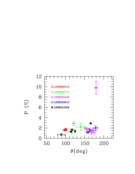
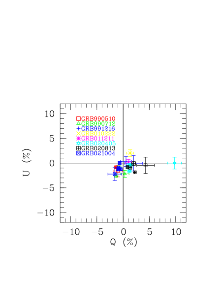
Figure 15: Summary of afterglow polarization measurement up to 2002 (from Covino, 2004). Top panel: degree of polarization and position angle for all the positive detections, i.e. upper limits are excluded. Bottom panel: Q and U Stokes parameters for all the available data, i.e. including upper limits.

The different predictions for the afterglow polarization light curves for different jet structures raise the hopes that afterglow polarization observations may constrain the jet structure. In practice, however, the situation is much more complicated, mainly since the observed polarization depends not only on the jet geometry, but also on the magnetic field configuration in the emitting region, which is not known very well. For example, an ordered magnetic field component in the emitting region (e.g. due to a small ordered magnetic field in the external medium) may dominate the polarized flux, and therefore the polarization light curves, even if it is sub-dominant in the emitting region compared to a random (shock generated) magnetic field component in terms of the total energy in the magnetic field (Granot & Königl, 2003). Other models for afterglow polarization include a magnetic field that is coherent over patches of a size comparable to that of causally connected regions (Gruzinov & Waxman, 1999), and polarization that is induced by microlensing (Loeb & Perna, 1998) or by scintillations in the radio (Medvedev & Loeb, 1999).

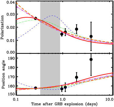
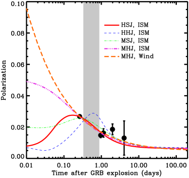
Figure 16: Fits of the predicted polarization for different jet structures and magnetic field configuration to the optical afterglow polarization data for GRB 020813 (from Lazzati et al., 2004). The upper panel shows the degree of polarization and position angle around the jet break time, which is also where the observations are concentrated, while the bottom panel shows the degree of polarization over a wider range in time and demonstrates that the differences between the various models are more pronounced at $t\lesssim t_{j}$. The shaded region denotes the allowed range for the jet break time $t_{j}$. The external density is taken to be either uniform (ISM, $k=0$) or a stellar wind (Wind, $k=2$). The different models are labeled by a three letter acronym where the first letter describes the magnetic field (‘H’ is for hydrodynamic, i.e. sock produced magnetic field, while ‘M’ is for magnetized, i.e. with an ordered toroidal magnetic field) while the second letter describes the jet structure (‘S’ for a structured jet, and ‘H’ for a homogeneous or uniform jet).

An additional complication arises in afterglow light curves that exhibit variability, since a variable afterglow light curve is expected to be accompanied by a variable polarization light curve, both in the degree of polarization and in its position angle (Granot & Königl, 2003). This prediction has been confirmed in GRB 021004 (Rol et al., 2003), where it had been interpreted both in the context of angular inhomogeneities within the jet (i.e. a “patchy shell”, Nakar & Oren, 2004) and as discrete episodes of energy injection into the afterglow shock (i.e. “refreshed shocks”, Björnsson, Gudmundsson & Jóhannesson, 2004), and later also in GRB 030329 (Greiner et al., 2003).

Perhaps the best monitored polarization light curve of a smooth afterglow, which does not suffer from the complications mentioned above, is GRB 020813 (Gorosabel et al., 2004) where the polarization position angle is roughly constant while the degree of polarization decreased by a factor of $\sim 2$ from $\sim 0.5t_{j}$ to $\sim 2t_{j}$. The constant position angle across the jet break time $t_{j}$ disfavors a uniform jet with a shock generated magnetic field (Sari, 1999; Ghisellini & Lazzati, 1999), as well as patches of uniform field (Gruzinov & Waxman, 1999) where the position angle (as well as the degree of polarization) is expected to change randomly on time scales $\Delta t\lesssim t$.

Lazzati et al. (2004) have contrasted different models for the jet structure and magnetic field configuration with the polarization data for GRB 020813 (see Figure 16), and concluded that the data support either (i) a structured jet (USJ) or a jet structure where most of the jet energy is in a narrow core while its wings contain less energy (such as a Gaussian jet) with a shock produced magnetic field (where the field is not purely in the plane of the shock but still possesses significant anisotropy) or (ii) a uniform jet with an ordered toroidal magnetic field component which dominates the polarized flux together with a random magnetic field component that dominates the total flux (and the total magnetic energy) in order for the polarization not to exceed the observed value.

We conclude that while the afterglow polarization light curves may provide useful constraints on the jet structure and the magnetic field configuration in the emitting region, it is in practice rather difficult to constrain each of these two ingredients separately. That is, in order to obtain tight constraints on the jet structure, strong assumptions must be made on the magnetic field configuration, and vice versa. Nevertheless, as discussed above, interesting constraints have already been derived from existing data.

0.3.4 Afterglow Light Curves

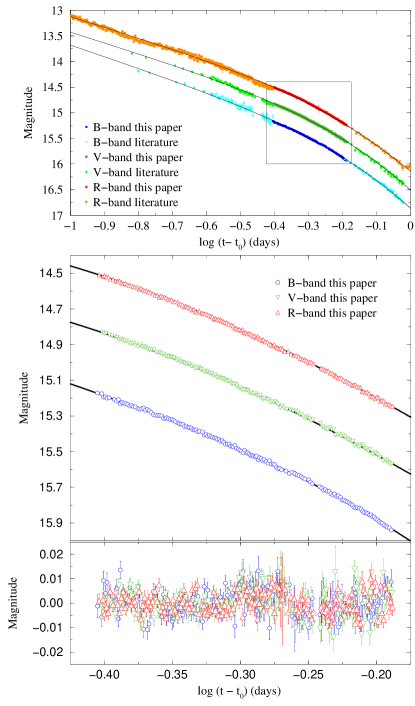
Figure 17: The jet break of GRB 030329 at three different optical bands, with exquisite temporal sampling (from Gorosabel et al., 2006). The upper panel shows a wider time span complemented by data from other groups, while the middle panel shows the data from Gorosabel et al. (2006), and the lower panel shows the residuals relative to a fit to a smooth jet break model. The steepening in the temporal decay during the jet break is smooth and achromatic.

The shape of the afterglow light curves is an important and relatively robust diagnostic tool for constraining the jet structure. The afterglow light curves (at least starting from a few hours after the GRB) are typically described by an initial power law flux decay $F_{\nu}\propto t^{-\alpha}$ with $0.7\lesssim\alpha_{1}\lesssim 1.5$ which steepens into a sharper power law decay ($1.6\lesssim\alpha_{2}\lesssim 2.8$) at the jet break time $t_{j}$ (Zeh, Klose & Kann, 2006). Figure 17 shows an example of the very well monitored jet break of GRB 030329. The jet break in the light curve is usually rather sharp (most of the steepening occurs within a factor of a few in time) and the increase in the temporal decay index, $\Delta\alpha=\alpha_{2}-\alpha_{1}$, is typically in the range $0.7\lesssim\Delta\alpha\lesssim 1.4$ (Zeh, Klose & Kann, 2006). Different jet structures may be tested by their ability to reproduce these observed properties. Below we describe the resulting constraints for various jet models.

Uniform Jet: Figure 18 shows the afterglow light curves for an initially uniform jet whose evolution is calculated using a hydrodynamic simulation (Granot et al., 2001). The initial conditions are a cone of half-opening angle $\theta_{0}$ taken out of the spherical self-similar Blandford & McKee (1976) solution (see §0.2.3). The shape of the light curves is nicely consistent with those observed in real afterglows, particularly in terms of the sharpness of the jet break, where the observed diversity can be attributed to different viewing angles within the jet aperture, $\theta_{\rm obs}<\theta_{0}$ (see upper panel of Figure 24).

Figure 18: Afterglow light curves for an initially uniform jet whose evolution is calculated using a hydrodynamic simulation, at different observe frequencies, for an observer along the jet symmetry axis (from Granot et al., 2001).

Gaussian Jet: the afterglow light curves for a Gaussian jet where $\epsilon(\theta)=\epsilon_{0}\exp(-\theta^{2}/2\theta_{c}^{2})$, that is observed at viewing angles inside the core of the jet ($\theta_{\rm obs}<\theta_{c}$) are rather similar to those for a uniform jet (Kumar & Granot, 2003; Rossi et al., 2004; Granot, Ramirez-Ruiz & Perna, 2005), and reasonably consistent with afterglow observations.

Structured Jet: one can consider a jet with a narrow core and wings where both $\epsilon$ and $\Gamma$ are initially power laws in the angle $\theta$ from the jet symmetry axis: $\epsilon\propto\theta^{-a}$ and $\Gamma_{0}\propto\theta^{-b}$, outside some (narrow) core angle $\theta_{c}$. A comparison between the resulting afterglow light curves and afterglow observations can then be used to constrain the power law indexes $a$ and $b$. Such an analysis (Granot & Kumar, 2003) suggests that $0\lesssim b\lesssim 1$ and $a\approx 2$ (or $1.5\lesssim a\lesssim 2.5$, see Figure 19).

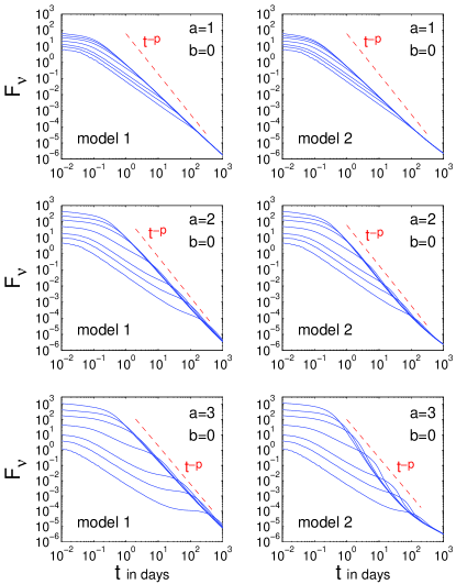
Figure 19: Afterglow light curves for a structured jet where initially $\epsilon\propto\theta^{-a}$ and $\Gamma\propto\theta^{-b}$ outside some core angle $\theta_{c}$ (from Granot & Kumar, 2003). The different curves, from top to bottom, are for viewing angles $\theta_{\rm obs}=0.01,\,0.03,\,0.05,\,0.1,\,0.2,\,0.3,\,0.5$, where $\theta_{c}=0.02$, $p=2.5$, $\epsilon_{e}=\epsilon_{B}=0.1$, $n_{\rm ext}=1\;{\rm cm^{-3}}$, $\Gamma(\theta=0,t_{0})=10^{3}$, and the total energy in the jet is $10^{52}\;$erg. In model 1 $\epsilon(\theta)$ does not change with time. In model 2, $\epsilon(\theta,t)$ evolves such that it is proportional to the average over its initial distribution, $\epsilon(\theta,t_{0})$, over the range in $\theta$ out to which a sound wave could propagate from $t_{0}$ up to $t$ (see Granot & Kumar, 2003, for details).

The upper limit on $b$ comes from the fact that a large value of $b$ implies a small initial Lorentz factor at large viewing angles, $\Gamma_{0}(\theta_{\rm obs}\gg\theta_{c})$, since it is hard for $\Gamma_{0}(\theta=0)$ to exceed $10^{4}$. A small initial Lorentz factor along the line of sight at large viewing angles would result in a large decelerations time along the line of sight and therefore an initially rising light curve, up to relatively late times, which is not seen in observations. Furthermore $\Gamma_{0}(\theta_{\rm obs})\gtrsim 100$ is needed in order to produce the prompt gamma-ray emission. Figure 19 shows light curves for $b=0$ and $a=1,\,2,\,3$ and different viewing angles. For $a=1$ the change in the temporal decay index across the jet break, $\Delta\alpha$, is too small (compared to its observed values) and the post-jet break decay slope is not steep enough. For $a=3$ there is either a very pronounced flattening in the light curve before the jet break time or the temporal decay slope after the jet break is extremely steep (neither of which is seen in afterglow observations). This suggests $a\approx 2$ (or $1.5\lesssim a\lesssim 2.5$).

As can be seen from Figure 20, even for $a=2$ and $b=0$ there is a flattening in the light curve before the jet break time, which becomes more pronounced at large viewing angles ($\theta_{\rm obs}\gg\theta_{c}$). This arises since the bright core of the jet becomes visible, while the value of $\epsilon$ along the line of sight is much smaller in comparison for large viewing angles, which more than compensates for the relatively small fraction of the visible region that is occupied by the jet core. That is, the average energy per solid angle in the observed region initially increases with time until the core of the jet becomes visible, and then decreases with time. Such a flattening has not been observed so for, but since it is most pronounced at large viewing angles for which the jet break time is large and the flux around that time is low, the observations in this parameter range are usually rather sparse, making it hard to rule out this model on these grounds.

Figure 20: Optical (R-band) light curves (upper panel) and the temporal decay index (lower panel) for a structured jet with no lateral spreading (from Rossi et al., 2004), for $a=2$, $b=0$, $E_{\rm k,iso}(\theta=0)=2\times 10^{54}\;$erg, $n_{\rm ext}=1\;{\rm cm^{-3}}$, $\epsilon_{e}=0.01$, $\epsilon_{B}=0.005$, $\theta_{c}=1^{\circ}$. The different curves are for different viewing angles, $\theta_{\rm obs}$, which are labeled in units of the jet core angle, $\theta_{c}$.

Two Component Jet Model: the light curves for this jet structure have been calculated analytically (Peng, Königl & Granot, 2005) or semi-analytically (Huang et al., 2004; Wu et al., 2005), and it has been suggested that this model can account for sharp bumps (i.e., fast rebrightening episodes) in the afterglow light curves of GRB 030329 (Berger et al., 2003b) and XRF 030723 (Huang et al., 2004). It has been later demonstrated, however, that effects such as the modest degree of lateral expansion that is expected in impulsive relativistic jets and the gradual hydrodynamic transition at the deceleration epoch smoothen the resulting features in the afterglow light curve, so that they cannot produce features as sharp as those mentioned above (Granot, 2005). One of the motivations for a two component jet was to alleviate the efficiency requirements on the prompt gamma-ray emission (Peng, Königl & Granot, 2005) if the wide jet dominates the total energy and late time afterglow emission, while the narrow jet is responsible for the prompt gamma-ray emission. However, the more recent Swift observations, which show a flat decay phase in the early X-ray afterglow (Nousek et al., 2006), are inconsistent which this picture and suggest a high gamma-ray efficiency also for this jet model under the standard assumptions of afterglow theory (Granot, Königl & Piran, 2006).

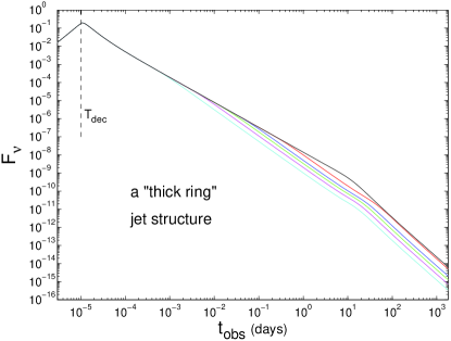
Figure 21: Light curves for a jet with an angular structure of a ring, where $\epsilon$ is uniform for $\theta_{c}<\theta<\theta_{c}+\Delta\theta$, and sharply drops outside of this range in $\theta$, for various fractional widths, viewed from within the jet. The upper line is for a uniform jet viewed from along its symmetry axis ($\theta_{c}=\theta_{\rm obs}=0$, $\Delta\theta=0.2$) and is included for comparison, while the other lines are for a ring shaped jet with $\theta_{c}=0.1$ and $\theta_{c}/\Delta\theta=1,\,2,\,3,\,5,\,10$, from top to bottom, viewed from $\theta_{\rm obs}=\theta_{c}+\Delta\theta/2$. A uniform external density ($k=0$), $p=2.5$, and no lateral expansion are assumed (from Granot, 2005).

Ring Shaped Jet: Figure 21 shows light curves for a ring shaped jet, viewed from within the emitting region, for different fractional width of the ring (Granot, 2005). For a thin ring, whose width is smaller than its radius, $\Delta\theta<\theta_{c}$, the jet break is divided into two distinct and smaller breaks, the first occurring when $\Gamma\Delta\theta\sim 1-2$ (i.e. when the width of the jet becomes visible) and the second when $\Gamma\theta_{c}\sim 1/2$ (i.e. when the whole jet becomes visible). This is inconsistent with the large steepening that is observed across the jet break, and suggests a “thick” ring, with $\Delta\theta\gtrsim\theta_{c}$. Even for such a thick ring with $\Delta\theta=\theta_{c}$ the jet break is still not quite sharp enough to match observations according to the model shown in Figure 21, however, the inclusion of some lateral expansion which would tend to smoothen the edges of the jet and fill in the center of the thick ring would probably be enough to make the light curve for $\Delta\theta\gtrsim\theta_{c}$ consistent with observed afterglow light curves. The fact that the beaming cone extends out to an angle of $\sim\Gamma^{-1}$ from the edge of the jet further contributes to smoothing the jet break for a thick ring jet, and contributes to the observed flux from lines of sight near the edge of the jet (Eichler, 2005).

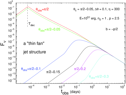
Figure 22: Light curves for a jet with an angular structure of a thin fan, with an opening angle of $\Delta\theta=0.1$ centered on $\theta=\pi/2$, i.e. $\theta_{c}=\pi/2-\Delta\theta/2=\pi/2-0.05$ (from Granot, 2005).

Fan Shaped Jet: Figure 22 shows the light curves for a jet in the shape of a thin fan, for different viewing angles. This jet structure is a limiting case of the ring shaped jet where $\theta_{c}=\pi/2-\Delta\theta/2$, and the jet occupies an angle of $\Delta\theta\ll 1$ centered around $\theta=\pi/2$. In this case the second jet break from the thin ring jet that had been discussed above occurs only when the jet becomes sub-relativistic, and is indistinguishable from the non-relativistic transition. This leaves only one jet break, when $\Gamma\Delta\theta\sim 1-2$ and the width of the jet becomes visible. The steepening in the flux decay rate across this jet break is at most half of that for a uniform jet (exactly half with no lateral expansion, and slightly less than half with rapid lateral expansion), and is too small compared to observations (Granot, 2005). This practically rules out a jet in the shape of a thin fan.

0.3.5 Off-Axis Viewing Angles

When the jet has relatively sharp edges, then the observed emission from viewing angles outside of the jet aperture is very different than that from viewing angles within the jet aperture (Panaitescu, Mészáros & Rees, 1998; Panaitescu & Mészáros, 1999; Moderski, Sikora & Bulik, 2000; Granot et al., 2001, 2002; Dalal, Griest & Pruit, 2002). If the line of sight is at an angle of $\Delta\theta_{\rm obs}$ outside the edge of the jet (i.e. from the nearest point in the jet with significant emission; for a uniform jet $\Delta\theta_{\rm obs}=\theta_{\rm obs}-\theta_{j}$) then at early times when $\Gamma\Delta\theta_{\rm obs}\gg 1$ the emitted radiation is strongly beamed away from the observer. This is since the emission is roughly isotropic in the comoving frame of the emitting material in the jet, and it is collimated within an angle of $\Gamma^{-1}$ around its direction of motion in the lab frame, due to relativistic beaming (i.e. aberration of light). As the jet decelerates, the beaming of radiation away from the line of sight becomes weaker, resulting in a rising flux. Eventually, when $\Gamma\Delta\theta_{\rm obs}$ decreases to $\sim 1$, the beaming cone of the jet encompasses the line of sight (see Figure 23) and the observed flux peaks and starts to decay, asymptotically joining the decaying light curve for viewing angles within the initial jet aperture.

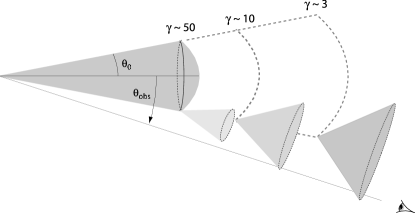
Figure 23: An illustrative diagram of the emission from a uniform relativistic jet with sharp edges and half-opening angle $\theta_{0}$, that is seen by an off-axis observer whose line of sight makes an angle $\theta_{\rm obs}>\theta_{0}$ with the jet axis. Because of relativistic beaming (i.e. aberration of light) the emission from each part of the jet is beamed into a narrow cone of half-opening angle $\gamma^{-1}$ around its direction of motion in the observer frame. During the prompt emission (and the very early afterglow) the Lorentz factor of the jet is large ($\gamma\gtrsim 50$) and therefore most of the radiation is strongly beamed away from the line of sight. In this case, the little radiation that is observed comes mainly from near the edge of the jet, at the point closest to the line of sight. As the jet decelerates $\gamma$ decreases with time and the beaming cone grows progressively wider, causing the radiation to be less strongly beamed, resulting in a rising light curve. The light curve peaks when $\gamma$ drops to $\sim(\theta_{\rm obs}-\theta_{0})^{-1}$ as the line of sight enters the beaming cone of the emitting material at the edge of the jet (the middle beaming cone in the figure), and subsequently decays with time, asymptotically approaching the light curve for an on-axis observer ($\theta_{\rm obs}<\theta_{0}$) at later times. (from Granot, Ramirez-Ruiz & Perna, 2005).

The afterglow light curves for different jet structures, dynamics, and viewing angles are shown in Figure 24. For an initially uniform jet with sharp edges whose evolution is calculated using a hydrodynamic simulation the rise to the peak in the light curve for viewing angles outside the initial jet aperture ($\theta_{\rm obs}>\theta_{0}$) is much more gradual compared to a semi-analytic model where the jet remains uniform with sharp edges and no lateral expansion. This is because of the mildly relativistic material at the sides of the jet whose emission is not strongly beamed away from such off-axis lines of sight ($\theta_{\rm obs}>\theta_{0}$) at early times, and therefore dominates the observed flux early on.

For a Gaussian jet, if both $\epsilon(\theta)$ and $\Gamma_{0}(\theta)$ have a Gaussian profile (corresponding to a constant rest mass per solid angle in the outflow), then the afterglow light curves are rather similar to those for a uniform jet (Kumar & Granot, 2003). If, on the other hand, $\epsilon(\theta)$ is Gaussian while $\Gamma_{0}(\theta)={\rm const}$, then the light curves for off-axis viewing angles (i.e., outside the core of the jet) have a much higher flux at early times, compared to a Gaussian $\Gamma_{0}(\theta)$ or a uniform jet (see the bottom two panels of Figure 24), due to a dominant contribution from the emitting material along the line of sight which has an early deceleration time in this case (Granot, Ramirez-Ruiz & Perna, 2005). Such a jet structure was considered as a quasi-universal jet model (Zhang et al., 2004).

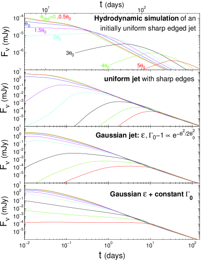
Figure 24: Afterglow light curves for different jet structures, dynamics, and viewing angles. The top panel is from an initially uniform jet with sharp edges whose evolution is calculated using a hydrodynamic simulation (taken from Figure 2 of Granot et al., 2002). The remaining three panels are taken from Figure 5 of Granot (2005), where a simplified jet dynamics with no lateral expansion is used. The second panel is for a uniform jet with sharp edges. The two bottom panels are for a Gaussian jet, in energy per solid angle, and either a Gaussian or a uniform initial Lorentz factor. The viewing angles are $\theta_{\rm obs}/\theta_{0}=0,\,0.5,\,1,\,1.5,\,2,\,3,\,4,\,5$, where $\theta_{0}$ is the (initial) half-opening angle for the uniform jet (two top panels) and the core angle ($\theta_{c}$) for the Gaussian jet (two bottom panels). (from Eichler & Granot, 2006).

It has been suggested that a uniform jet with sharp edges viewed from slightly outside of its edge ($\theta_{0}<\theta_{\rm obs}\lesssim 2\theta_{0}$) would result in an X-ray flash (XRF) or X-ray rich GRB (XRGRB) (Yamazaki, Ioka & Nakamura, 2002, 2003, 2004), because of the smaller blue-shift of the prompt emission compared to viewing angles within the jet ($\theta_{\rm obs}<\theta_{0}$). This has also been found to nicely explain the flat early part of the light curve of XRGRB 041006 with $(\theta_{\rm obs}-\theta_{0})\sim 0.15\theta_{0}$ and XRF 030723 with $(\theta_{\rm obs}-\theta_{0})\sim\theta_{0}$ (Granot, Ramirez-Ruiz & Perna, 2005, see Figure 25), as naturally expected in this model, since a larger angular displacement outside the edge of the jet should result in a softer prompt emission. There is a good case for a viewing angle slightly outside the edge of a uniform sharp edged jet also in the case of GRB 031203 (Ramirez-Ruiz et al., 2005, see Figure 26).

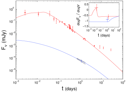
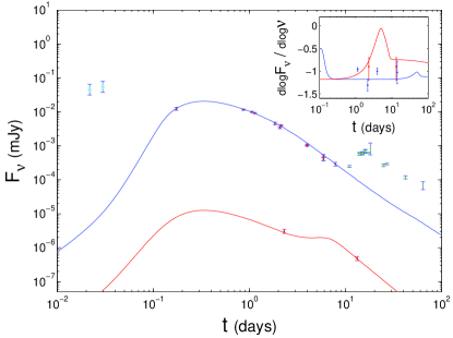
Figure 25: Tentative fits to the afterglow light curves of X-ray rich GRB 041006 (upper panel) and X-ray flash XRF 030723 (lower panel) for a uniform sharp edged jet with a constant half-opening angle $\theta_{0}$, viewed from an angle $\theta_{\rm obs}$ slightly outside of its edge, with $(\theta_{\rm obs}-\theta_{0})\sim 0.15\theta_{0}$ for XRGRB 041006 and $(\theta_{\rm obs}-\theta_{0})\sim\theta_{0}$ for XRF 030723 (for details see Granot, Ramirez-Ruiz & Perna, 2005). In both panels the upper curve is optical (R-band) and the lower curve is X-rays ($0.5-6\;$keV for XRGRB 041006 and $0.5-8\;$keV for XRF 030723), while the inset shows the optical and X-ray spectral slopes.

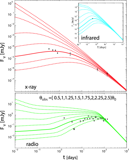
Figure 26: A tentative fit to the afterglow light curve of GRB 031203 with a uniform sharp edged jet of half-opening angle $\theta_{0}=5^{\circ}$ for different viewing angles $\theta_{\rm obs}$ from its symmetry axis (from Ramirez-Ruiz et al., 2005).

This expectation arises, however, assuming that the regions of prominent gamma-ray emission and afterglow emission coincide. If this assumption is relaxed (Eichler & Granot, 2006), then an initially flat light curve may appear in hard and bright GRBs, for lines of sight along which there is bright gamma-ray emission but hardly any afterglow emission. In this picture viewing angles outside the region within the jet with bright afterglow emission can naturally account for the early flat part of the X-ray afterglows detected by Swift (Nousek et al., 2006). These early flat decay stages cannot be attributed to viewing angle effects in the USJ model, where there is always significant afterglow emission along the line of sight. In scenarios where a break in the light curve is caused by the jet structure and/or dynamics, the break is expected to be largely achromatic.

0.3.6 Orphan Afterglows

For a jet with reasonably sharp edges, the prompt GRB emission becomes very dim at viewing angles significantly outside the edge of the jet ($\Gamma\Delta\theta_{\rm obs}\gg 1$), and it can therefore be detected only from within or slightly outside the initial jet aperture, $\Gamma_{0}(\theta_{\rm obs}-\theta_{0})\lesssim{\rm a\ few}$. From larger viewing angles the prompt emission would not be detected. During the afterglow, however, the jet decelerates and its beaming cone widens with time, so that the afterglow emission at late times can become detectable out to much larger viewing angles. Such events, with no detected prompt GRB emission but with detected afterglow emission in lower frequencies at later times, are called orphan afterglows. While no such orphan afterglow has been detected to date, their potential for constraining the degree of collimation of the jet has been realized early on (Rhoads, 1997).

In addition to “off-axis” orphan afterglows, where the prompt emission is not detected due to a viewing angle outside of the jet, there can also be “on-axis” orphan afterglows, where there is significant afterglow emission along the line of sight from relatively early times, but for some reason the prompt gamma-ray emission along the line of sight is very weak (Huang, Dai & Lu, 2002; Nakar & Piran, 2003). This could occur, for example, if the initial Lorentz factor along the line of sight is not large enough to avoid excessive pair production (the “compactness” problem), $\Gamma_{0}\lesssim 100$, while it is still sufficiently large in order for the deceleration time $t_{\rm dec}$ to be early enough to enable the detection of the afterglow emission (typically $t_{\rm dec}\lesssim 1\;$day for $\Gamma_{0}\gtrsim 10$).

Many works have analyzed the expected detection rate of orphan afterglows, as well as the constraints on the degree of collimation of GRB jets from existing surveys, in the X-ray (Woods & Loeb, 1999; Nakar & Piran, 2003), optical (Dalal, Griest & Pruit, 2002; Totani & Panaitescu, 2002; Nakar, Piran & Granot, 2002; Rhoads, 2003; Rau, Greiner & Schwartz, 2006), and radio (Perna & Loeb, 1998; Levinson et al., 2002; Gal-Yam et al., 2006). The constraints derived in this way are still not very severe, but are nevertheless becoming increasingly more interesting. Future surveys for orphan afterglows in the X-ray, optical and radio can help constrain the degree of collimation of GRB jets, as well as the jet structure. The detection of orphan GRB afterglows would provide an important independent line of evidence in favor of jets in GRBs.

0.3.7 Some Implications of recent Swift Observations

The ability of the Swift satellite to rapidly and autonomously slew toward GRBs and observe them in X-rays, UV, and optical, has dramatically improved our knowledge of the early afterglow emission. In particular it provided excellent coverage of the early X-ray afterglow, and enable rapid followup observations in the optical and NIR by ground based robotic telescopes. In the context of jets, there are two main new observations which are most relevant.

The first is the lack of a clear jet break in the afterglow light curve of most Swift GRBs. Even when a break in the light curve does show up, it is often chromatic (Panaitescu et al., 2006), i.e. seen in the X-rays but not in the optical, in stark contrast with the largely achromatic nature that is expected for a jet break. The lack of a clear jet break in many Swift GRBs can at least in part be attributed to the larger sensitivity of Swift compared to previous missions, that causes it to detect dimmer GRBs on average, which in turn correspond to wider jets with a later jet break time and lower flux at that time, making it harder to observe a clear jet break. It is not yet clear whether this explanation can fully account for paucity of clear jet breaks in Swift GRBs. Furthermore, the chromatic breaks that are seen in the afterglow light curves of some Swift GRBs definitely require a novel explanation.

The second new Swift observation that bears relevance for the efficiency of the prompt gamma-ray emission, $\epsilon_{\gamma}$, and for the kinetic energy, $E_{k}$, of the jet during the late phases of the afterglow for different jet structures (following Granot, Königl & Piran, 2006), is the flat decay phase in the early X-ray afterglow of many Swift GRBs. Pre-Swift studies (Panaitescu & Kumar, 2002; Yost et al., 2003; Lloyd-Ronning & Zhang, 2004) found that the isotropic equivalent kinetic energy in the the afterglow shock at late times (typically evaluated at $t=10\;$hr), $E_{\rm k,iso}(10\;{\rm hr})$, is comparable to the isotropic equivalent energy output in gamma rays, $E_{\rm\gamma,iso}$, i.e. that typically $\kappa\equiv E_{\rm\gamma,iso}/E_{\rm k,iso}(10\;{\rm hr})\sim 1$. The gamma-ray efficiency is given by $\epsilon_{\gamma}=E_{\rm\gamma,iso}/(E_{\rm\gamma,iso}+E_{\rm k,iso,0})$, where $E_{\rm k,iso,0}$ is the initial value of $E_{\rm k,iso}$ corresponding to material with a sufficiently large initial Lorentz factor ($\Gamma_{0}\gtrsim 10^{2}$) that could have contributed to the prompt gamma-ray emission. This implies a simple relation, $\epsilon_{\gamma}/(1-\epsilon_{\gamma})=\kappa f$, where $f\equiv E_{\rm k,iso}(10\;{\rm hr})/E_{\rm k,iso,0}$ can be estimated from the early afterglow light curve.

If the flat decay phase in the early X-ray afterglow observed by Swift is interpreted as energy injection (Nousek et al., 2006; Zhang et al., 2006; Panaitescu et al., 2006; Granot & Kumar, 2006) this typically implies $f\gtrsim 10$ and therefore $\epsilon_{\gamma}\gtrsim 0.9$. This is a very high efficiency for any reasonable model for the prompt emission, and in particular for the popular internal shocks model. If the early flat decay phase is not due to energy injection, but is instead due to an increase with time in the afterglow efficiency, then $f\sim 1$ and typically $\epsilon_{\gamma}\sim 0.5$. This is a more reasonable efficiency, but still rather high for internal shocks. Such an increase in the afterglow efficiency can occur, e.g., if one or more of the following shock micro-physics parameters increases with time: the fraction of the internal energy in relativistic electrons, $\epsilon_{e}$, or in magnetic fields, $\epsilon_{B}$, or the fraction $\xi_{e}$ of the electrons that are accelerated to a relativistic power-law distribution of energies. If, in addition, $E_{\rm k,iso}(10\;{\rm hr})$ had been underestimated, e.g. due to the assumption that $\xi_{e}=1$, then $\kappa\sim\xi_{e}$ and $\xi_{e}\sim 0.1$ would lead to $\kappa\sim 0.1$ and $\epsilon_{\gamma}\sim 0.1$.

The internal shocks model can reasonably accommodate gamma-ray efficiencies of $\epsilon_{\gamma}\lesssim 0.1$, which in turn imply $\kappa\lesssim 0.1$. Since the true (corrected for beaming) energy output in gamma rays, $E_{\gamma}=f_{b}E_{\rm\gamma,iso}$ where $f_{b}=(1-\cos\theta_{0})\approx\theta_{0}^{2}/2$, is clustered around $10^{51}\;$erg (Frail et al., 2001; Bloom, Frail & Kulkarni, 2003), this implies $E_{k}(10\;{\rm hr})=f_{b}E_{\rm k,iso}(10\;{\rm hr})=E_{\gamma}/\kappa\gtrsim 10^{52}\;$erg for a uniform jet. For a structured jet with equal energy per decade in $\theta$ ($\epsilon\propto\theta^{-2}$) in the wings, the true energy in the jet is larger by a factor of $1+2\ln(\theta_{\rm max}/\theta_{c})\sim 10$, which implies $E_{k}(10\;{\rm hr})\gtrsim 10^{53}\;$erg in order to achieve $\epsilon_{\gamma}\lesssim 0.1$. Such energies are comparable (for the UJ model) or even higher (for the USJ model) than the estimated kinetic energy of the Type Ic supernova (or hypernova) that accompanies the GRB. This is very interesting for the total energy budget of the explosion.

0.4 Summary and Conclusions

Our current understanding of GRB jets has been reviewed with special emphasis on the jet dynamics (§0.2) and structure (§0.3). The main conclusions are as follows. Semi-analytic models predict a very rapid sideways expansion of the jet once its Lorentz factor drops below the inverse of its initial half-opening angle (§0.2.1). Numerical studies, however, show a very modest degree of lateral expansion as long as the jet is relativistic. Such numerical studies include both an intermediate approach where the hydrodynamic variables are integrated over the radial profile of the jet, which significantly simplifies the hydrodynamic equations (§0.2.2), and full hydrodynamic simulations (§0.2.3).

The full hydrodynamic simulations are the most reliable of these methods. The fact that the result of the intermediate method (described in §0.2.2) for an initially Gaussian jet agree rather well with hydrodynamic simulations of an initially uniform jet with sharp edges, lends credence to its results, which show that also for a “structured” jet the lateral expansion is very small (even smaller than for an initially uniform or Gaussian jet, because of the smaller gradients in the lateral direction) and the distribution of energy per solid angle remains very close to its initial form as long as the jet is relativistic.

The afterglow image is expected to be rather uniform at low frequencies (radio) and more limb brightened at higher frequencies (optical, UV or X-rays). Its morphology and the evolution of its size can help probe the jet dynamics and structure, as well as the external density profile (§ 0.2.5).

The observed jet break in the light curve in a uniform jet occurs predominantly due to the lack of contribution to the observed flux from outside the edges of the jet, once they become visible, and the very modest lateral expansion does not play an important role (§0.2.6).

The most popular models for the jet structure are the uniform jet (UJ) model, where the jet is uniform within some finite half-opening angle and has sharp edges, and the universal structured jet (USJ) model, where the jet has a narrow core and wings where the energy per solid angle drops as a power law (usually assumed to be an inverse square) with the angle from the jet symmetry axis. There are also other jet structures that have been discussed in the literature, which include a Gaussian jet, a two component jet with a narrow uniform core of initial Lorentz factor $\Gamma_{0}\gtrsim 10^{2}$ surrounded by a wider uniform component with $\Gamma_{0}\sim 10-30$, and jets with a cross section in the shape of a ring (or “hollow cone”) or a fan (see Figure 13).

There are various approaches for constraining the jet structure. Statistical studies of the prompt emission are not very conclusive yet, while the observed combined distribution of jet break times and redshifts appears to disfavor the USJ model (§0.3.2). The evolution of the linear polarization of the afterglow provides interesting constraints on the jet structure and the magnetic field configuration in the emitting region (§0.3.3), but it is difficult to obtain tight constraints on the jet structure without making strong assumptions about the magnetic field configuration.

The shape of the afterglow light curves is an important and relatively robust diagnostic tool for constraining the jet structure (§0.3.4). It can practically rule out a jet with a cross section of a narrow ring or a fan, and it constrains the properties of a two component jet. The light curves for viewing angles slightly outside the (reasonably sharp) edge of a jet would initially rise or at least be very flat before they join the decaying light curve for lines of sight within the (initial) jet aperture (§0.3.5). This can naturally account for such a flat decay phase observed in the best monitored pre-Swift X-ray flash (030723) and X-ray rich GRB (041006). It can also explain the early X-ray afterglow light curves of many Swift GRBs if the regions of prominent gamma-ray and afterglow emission do not coincide (Eichler & Granot, 2006). However, this cannot be attributed to viewing angle effects in the USJ model, while in the Gaussian jet model it suggests that the initial Lorentz factor significantly drops outside of the jet core.

Our understanding of the structure and dynamics of GRB jets may improve thanks to future observations. These include a dense monitoring of the afterglow emission starting at early times and over a wide range of frequencies (radio, mm, NIR, optical, UV, X-ray), polarization measurements with good temporal coverage both at early times (much earlier than the jet break time) and around (i.e. at least a factor of a few before and after) the jet break time, and measuring the evolution of the afterglow image size. Surveys for orphan afterglows (§0.3.6) are already beginning to provide interesting constraints on the collimation of GRB jets, and future surveys may also constrain the jet structure. The detection of orphan GRB afterglows may also provide an important independent line of evidence for jets in GRBs. Recent Swift observations (§0.3.7) show a paucity of clear achromatic jet breaks in the afterglow light curves as well as chromatic breaks which challenge existing models and call for new explanations.