The build–up of the colour–magnitude relation in galaxy clusters since $z\sim 0.8$

Abstract

Using galaxy clusters from the ESO Distant Cluster Survey, we study how the distribution of galaxies along the colour–magnitude relation has evolved since $z\sim 0.8$. While red–sequence galaxies in all these clusters are well described by an old, passively evolving population, we confirm our previous finding of a significant evolution in their luminosity distribution as a function of redshift. When compared to galaxy clusters in the local Universe, the high redshift EDisCS clusters exhibit a significant deficit of faint red galaxies. Combining clusters in three different redshift bins, and defining as ‘faint’ all galaxies in the range $0.4\,\gtrsim\,$L$/$L${}_{*}\,\gtrsim\,0.1$, we find a clear decrease in the luminous–to–faint ratio of red galaxies from $z\sim 0.8$ to $z\sim 0.4$. The amount of such a decrease appears to be in qualitative agreement with predictions of a model where the blue bright galaxies that populate the colour–magnitude diagram of high redshift clusters, have their star formation suppressed by the hostile cluster environment. Although model results need to be interpreted with caution, our findings clearly indicate that the red–sequence population of high–redshift clusters does not contain all progenitors of nearby red–sequence cluster galaxies. A significant fraction of these must have moved onto the red–sequence below $z\sim 0.8$.

1 Introduction

Galaxy clusters may be considered as laboratories for studying the physical processes that drive galaxy evolution. They offer the possibility to trace the properties of galaxies in similar environments over a relatively long time baseline. In addition, they offer the practical advantage of providing many galaxies in a relatively small region of the sky and all approximately at the same redshift. This allows efficient observation even with modest fields of view and modest amounts of telescope time. It should be noted, however, that in order to establish that physical processes related to the cluster environment are indeed playing a role, it is necessary to compare the evolution of similar galaxies in different environments (i.e. in the clusters and in the ‘field’). In addition, galaxy clusters represent a biased environment for evolutionary studies. In the current standard cosmogony, clusters originate from the gravitational collapse of the highest (and rarest) peaks of primordial density perturbations, and evolutionary processes in these regions occur at an accelerated pace with respect to regions of the Universe with average density.

The technical capabilities achieved in recent years have provided a rapidly growing database on high–redshift clusters (Zaritsky et al., 1997; Gonzalez et al., 2001; Valtchanov et al., 2004; Gladders & Yee, 2005; Kodama et al., 2005; White et al., 2005; Wilson et al., 2006). These, interpreted using the latest theoretical techniques (Cole et al., 2000; Hatton et al., 2003; Springel et al., 2005; De Lucia et al., 2006), should provide important constraints on the physical mechanisms driving the formation and the evolution of cluster galaxies.

Early studies of the galaxy population in distant clusters pointed out significant differences with respect to nearby systems (Butcher & Oemler, 1984). More recent work has provided us with a much more detailed picture of these differences (a very incomplete list of recent papers includes Stanford et al., 2005; Postman et al., 2005; Jørgensen et al., 2005; White et al., 2005; Poggianti et al., 2006; Strazzullo et al., 2006). One interesting outcome of these studies has been the discovery that a tight relation between the colours and the magnitudes of bright elliptical galaxies holds up to the highest redshifts probed so far (Blakeslee et al., 2003; De Lucia et al., 2004; Holden et al., 2004; Mei et al., 2006).

The existence of a colour–magnitude relation (hereinafter CMR) has been known for a long time (de Vaucouleurs, 1961; Visvanathan & Sandage, 1977). At least in nearby clusters (de Propris et al., 1998), it appears to extend $5-6$ mag faint-ward of the Brightest Cluster Galaxy (BCG). At the present epoch, the CMR can be interpreted either as a result of differing ages (bluer galaxies being younger), or of differing metallicities (bluer galaxies being more metal poor), or as a combination of the two (Ferreras, Charlot & Silk 1999; Terlevich et al., 1999; Poggianti et al., 2001a, and references therein).

The mere existence of a tight relation at high redshift favours the metallicity interpretation and naively appears to make the age explanation untenable. The reason for this is that if one assumes that all present–day red–sequence galaxies are still identified as red–sequence members in high–redshift clusters, then if the CMR were primarily age driven it would change dramatically with increasing redshift as small galaxies approach their formation epoch and progressively become brighter and bluer (Kodama et al., 1998). This expectation is in contrast with observational results which show that the slope of the CMR does not change appreciably over the redshift interval $0-1$ (Gladders et al., 1998; Stanford et al., 1998, and more recent work mentioned above).

One possible simple interpretation is then that cluster elliptical galaxies represent a passively evolving population formed at high-redshift (z $>2-3$) in a short duration event (but see the discussion by Bower, Kodama & Terlevich, 1998). In this scenario – often referred to as monolithic – the CMR arises through the effects of supernovae winds: supernovae explosions heat the interstellar medium triggering galactic winds whenever the thermal energy of the gas exceeds its gravitational binding energy. Since smaller galaxies have shallower potential wells, this results in greater mass loss by smaller systems, naturally establishing the observed CMR. A difficulty may be that the observed CMR shows no sign of a turnover at high mass of the kind predicted by such models (Larson, 1974).

This simple model may be too naive for explaining the origin and the evolution of the observed CMR. In the monolithic scenario a galaxy has a single well–defined progenitor at each redshift and its evolution is described by simple smooth functions of time. This is not true in the current standard cosmological paradigm, where a single galaxy today corresponds to the ensemble of all its progenitors at any previous redshift (see discussion in De Lucia & Blaizot, 2006). It is not obvious then that high–redshift red-sequence galaxies contain all or even most of the progenitors of nearby red–sequence cluster galaxies. Indeed the results we present below give direct evidence that this is not the case. In addition, the simple model described above, clearly neglects the infall of “new” galaxies during cosmological growth of the cluster. If the intra-cluster environment is associated with suppression of star formation, then these galaxies would become redder and fainter and might also join the red–sequence galaxy population at lower redshifts.

An alternative scenario has been proposed by Kauffmann & Charlot (1998) - see also De Lucia, Kauffmann & White (2004) - in the framework of hierarchical models of galaxy formation. In these models, the CMR arises as a result of the fact that more massive ellipticals originate from the mergers of more massive - and more metal–rich - disk systems. The models show a well defined red–sequence, still mainly driven by metallicity differences, that is in place up to redshift $\sim 2$, although with a scatter that is larger than that observed.

Recent work on the observed colour–magnitude relation of high–redshift clusters has pointed out a new and still controversial result concerning an apparent ‘truncation’ of the CMR at redshift about $0.8$ (De Lucia et al., 2004; Kodama et al., 2004).

In De Lucia et al. (2004), we analysed the colour–magnitude relation of $4$ clusters in the redshift interval $0.7$–$0.8$ from the ESO Distant Cluster Survey (hereinafter EDisCS) and found a deficiency of low luminosity passive red galaxies with respect to the nearby Coma cluster. A decrease in the number of faint red galaxies was detected in all clusters under investigation but one (with low number of cluster members), although the significance of the deficit was only at about the $3\sigma$ level. In this paper we extend our analysis to the full EDisCS sample covering the redshift range $0.4-0.8$ and a wide range of structural properties. The plan of the paper is as follows. The observational data used for our study are briefly described in Sec. 2. In Sec. 3 we present the criteria used to define cluster membership and in Sec. 4 we present the colour–magnitude relation for all the clusters in the EDisCS sample. In Sec. 5 we study the distribution of galaxies along the red–sequence, and discuss its dependence on redshift and on cluster velocity dispersion. The red–sequence galaxy distribution in nearby clusters is studied in Sec. 6. In Sec. 7, we interpret the evolution measured as a function of redshift in terms of simple population synthesis models. Finally, in Sec. 8, we discuss our results and give our conclusions.

Throughout this paper we will assume a $\Lambda$CDM cosmology: $H_{0}=70\,{\rm km}\,{\rm s}^{-1}\,{\rm Mpc}^{-1}$, $\Omega_{\rm m}=0.3$ and $\Omega_{\Lambda}=0.7$. With this cosmology, $z\sim 0.8$ - the highest redshift probed by our cluster sample - corresponds to more that $50$ per cent of the look-back time to the Big Bang. Throughout this paper we use Vega magnitudes, unless otherwise stated.

2 The data

EDisCS is an ESO Large Programme aimed at the study of cluster structure and cluster galaxy evolution over a significant fraction of cosmic time. The complete EDisCS dataset provides homogeneous photometry and spectroscopy for $20$ fields containing galaxy clusters at $z=0.4$–$1$. Clusters candidates were selected from the Las Campanas Distant Cluster Survey (LCDCS) of Gonzalez et al. (2001) by identifying surface brightness excesses using a very wide filter ($4500$–$7500$ Å) in order to maximise the signal-to-noise of distant clusters against the sky. The EDisCS sample of $20$ clusters was constructed selecting $30$ from the highest surface brightness candidates in the LCDCS, and confirming the presence of an apparent cluster and of a possible red sequence with VLT $20$min exposures in two filters. From these $30$ candidates, we then followed up $10$ among the highest surface brightness clusters in the LCDCS in each of the ranges of estimated redshift $0.45<z_{\rm est}<0.55$ and $0.75<z_{\rm est}<0.85$. In the following, we will often refer to these as the intermediate and high redshift samples respectively.

As a consequence of the scatter of the estimated redshifts about the true value, we have ended up with a set of clusters distributed relatively smoothly between $z=0.42$ and $z=0.96$, rather than two samples concentrated at $0.5$ and $0.8$, as originally planned. Details on the selection of cluster candidates can be found in White et al. (2005). Our follow-up programme obtained deep optical photometry with FORS2/VLT (White et al., 2005), near-IR photometry with SOFI/NTT (Aragón-Salamanca et al. in preparation), and multislit spectroscopy with FORS2/VLT for the $20$ fields (Halliday et al. 2004; Milvang-Jensen et al. in preparation). ACS/HST mosaic imaging of $10$ of the highest redshift clusters has also been acquired (Desai et al. in preparation). For three EDisCS clusters, narrowband $H_{\alpha}$ imaging has been acquired (Finn et al., 2005) and for three clusters we have XMM data (Johnson et al., 2006).

The optical ground–based photometry and a first basic characterisation of our sample of clusters as a whole, is presented in White et al. (2005). In brief, our optical photometry consists of V, R, and I imaging for the $10$ highest redshift cluster candidates and B, V, and I imaging for the remaining $10$ intermediate redshift cluster candidates. Total integration times were typically $45$ minutes at the lower redshift and $2$ hours at the higher redshift. Object catalogues have been created using the SExtractor software version 2.2.2 (Bertin & Arnouts, 1996) in ‘two–image’ mode using the I–band images as detection reference images. Magnitudes and colours have been measured on the seeing–matched images (to $0\aas@@fstack{\prime\prime}8$ – the typical seeing in our IR images) using fixed circular apertures. Throughout this paper, we correct magnitudes and colours for Galactic extinction according to the maps of Schlegel, Finkbeiner & Davis (1998) and a standard Milky Way reddening curve. We refer to White et al. (2005) for details about our photometry. In the following, we will use magnitudes and colours measured using a fixed circular aperture with $1\aas@@fstack{\prime\prime}0$ radius. This choice has been adopted to simplify the comparison with the Coma cluster, as we will explain later in the paper. The cluster velocity dispersions and ${\rm R}_{200}$ we use in the following are the same as used in Poggianti et al. (2006) and are listed in Table 1 of that paper.

As a part of our programme, we also obtained spectra for $>100$ galaxies per cluster field (typical exposure times were $4$ hours for the high redshift candidates and $2$ hours for the intermediate redshift clusters). The spectroscopic selection, observations, data reduction, and spectroscopic catalogues are presented in Halliday et al. (2004) and Milvang-Jensen et al. (in preparation). As explained in White et al. (2005), deep spectroscopy was not obtained for two of the EDisCS fields (cl$1122.9$-$1136$ and cl$1238.5$-$1144$), which are not included in the present study.

3 Cluster membership

Although complications arise from the existence of redshift space distortions, spectroscopic redshifts provide the optimal technique to determine cluster membership. However, obtaining spectroscopic redshifts for large numbers of faint objects is not feasible within the available time with current instrumentation, even for samples just beyond $z=0.5$. A standard method to correct for field contamination, in absence of spectroscopy, is to use statistical field subtraction (Aragón-Salamanca et al., 1993; Stanford et al., 1998; Kodama & Bower, 2001): a ‘cluster–free’ field is used to determine the number of contaminating galaxies as a function of magnitude and/or colour. This method becomes increasingly uncertain at high redshift: Driver et al. (1998), for example, used simulations to show that it is already unreliable at $z>0.3$. In addition, this approach does not provide the likelihood of being a cluster member on a galaxy–by–galaxy basis.

In the last decade, the techniques used to determine photometric redshifts have become much more precise, suggesting that they can be used to address specific scientific questions (Benítez, 2000; Bolzonella et al., 2000; Rudnick et al., 2001; Firth et al., 2003). An important by–product is an estimate of the spectral type for each observed galaxy. Errors in estimated photometric redshifts are much larger than typical errors in spectroscopic redshifts. In addition, systematics or degeneracies are often present because of uncertainties in the redshift evolution of spectral energy distributions and/or insufficient calibrating spectroscopy for the magnitude range sampled by the photometric data.

Given the difficulties mentioned above, we decided in the present study to use both a ‘classical’ statistical field subtraction and a membership criterion based on photometric redshift information. We give a brief description of both methods in the following sections.

3.1 Photometric redshifts

Photometric redshifts were computed using two different codes (Bolzonella et al., 2000; Rudnick et al., 2001) in order to provide better control of the systematics in the identification of likely non–members. The two codes employed in this study are based on the use of similar SED fitting procedures, but different template spectra, different minimisation algorithms, and a number of other different details (see the original papers). The performance of these codes on the EDisCS dataset will be examined in Pelló et al. (in preparation).

For the purposes of this analysis, the codes were run allowing a maximum photometric redshift of $2$ and assuming a $5$ per cent minimum flux error for the photometry. Where they can be checked, the photometric redshifts of the galaxies in our sample are quite accurate with $<|z_{\rm spec}-z_{\rm phot}|>=0.06$–$0.08$. There is no systematic trend between $z_{\rm phot}-z_{\rm spec}$ and $z_{\rm spec}$ and the percentage of catastrophic failures, i.e. the fraction of objects with $|z_{\rm spec}-z_{\rm phot}|>0.3$, is of the order of $10$ per cent.

In the present study, we use the redshift probability distributions provided by the two photometric redshift codes, as a quantitative tool to estimate cluster membership. Briefly, we accept galaxies as potential cluster members if the integrated probability for the photometric redshift to be within $\pm\,0.1$ of the (known) cluster redshift is greater than a specific threshold for both of the photometric redshift codes. These probability thresholds (${\rm P}_{\rm thresh}$) range from $0.1$ to $\,0.35$, depending on the filter set available for each particular field, and they were calibrated using our spectroscopy to maximise the cluster membership and, at the same time, to minimise contamination from interlopers.

Calibration against our spectroscopic sample shows that this technique allows us to retain more than $90$ per cent of the cluster members while rejecting slightly less than $50$ per cent of the non–members in the spectroscopic sample. The efficiency of rejection for the bluest and reddest halves of the sample is similar to within less than $10$ per cent. However, red non–members are slightly more efficiently rejected, and red members slightly more efficiently accepted than their blue counterparts at identical ${\rm P}_{\rm thresh}$. This is expected because of the poorer constraints on $z_{\rm phot}$ for blue galaxies due to their smoother SEDs.

A method similar to that used in our study was proposed by Brunner & Lubin (2000). Their application was based on the use of an “empirical” photometric redshift technique. The latter is based on the use of an empirical relation, measured for the spectroscopic sample available, between the spectroscopic redshifts and the photometric data points. The use of this method, forced Brunner & Lubin to assume a probability distribution, which they supposed to be Gaussian with mean given by the estimated photometric redshift and standard deviation defined by the estimated error. The error distributions are, however, usually strongly non–Gaussian (Rudnick et al., 2001), so proper use of the probability distributions provides a better estimate of the real uncertainty in the photometric redshift estimates.

When available, we use the spectroscopic information to determine cluster membership: spectroscopic non-members that are erroneously classified as cluster members by the photometric redshift criterion detailed above, are rejected. Spectroscopic members that are erroneously rejected are re-included into the sample before the analysis. The photometric redshift technique we use performs well, particularly on red galaxies. As a consequence, this latter correction based on the availability of spectroscopic information, does not modify significantly the results discussed below. We note that spectroscopic membership has been defined as in Halliday et al. (2004). The number of spectroscopic members for our clusters ranges from $11$ to $67$ (see Table 1 in Poggianti et al., 2006). If membership is assigned using the photometric redshift method outlined above, the fraction of cluster members for which spectra are available ranges from a few to about $15$ per cent.

3.2 Statistical subtraction

As an alternative method to determine cluster membership, we employ a ‘classical’ statistical subtraction technique. The method we use is similar to that adopted in Pimbblet et al. (2002). We refer to the original paper for more details on the procedure which we only briefly outline here.

The ‘field’ population has been determined from one field of the Canada France Deep Field Survey (McCracken et al., 2001). This corresponds to an area of about $0.25\,$deg², which is much larger than the cluster area used for our analysis (see next section). Both the cluster and the field regions are binned onto a gridded colour–magnitude diagram (we use a $0.3$ bin in colour and a $0.5$ bin in magnitude). The field region is then scaled to the same area as the cluster region we wish to correct, and each galaxy is assigned a probability to be a cluster member simply by counting how many galaxies lie in the colour–magnitude bin in the two different regions. Using a Monte Carlo method, the field population is then subtracted off. If this procedure gives a negative number of galaxies in the cluster population at a particular grid position, the mesh size is increased for that particular position. As explained in Appendix A of Pimbblet et al. (2002), this approach has the advantage of preserving the original probability distribution better than similar methods (Kodama & Bower, 2001) where the excess probability is distributed evenly between the neighbours of critical grid positions. For each cluster we run $100$ Monte Carlo realizations of the above procedure.

When available, we use the spectroscopic information: spectroscopic members and non-members are always assigned a probability $1$ and $0$ to be cluster members respectively. As is the case when cluster membership is assigned using photometric redshifts, this correction does not modify significantly the results presented below.

4 The colour–magnitude relation

Figure 1: Colour–magnitude diagrams for the $18$ EDisCS fields used in this study. Empty circles show objects retained by our photometric redshift criterion. Blue and red filled circles represent spectroscopically confirmed members with and without emission lines in their spectra. Thin slanted lines correspond to the $1$, $3$ and $5\sigma$ detection limits in the V-band. The solid thick line in each panel, represents the best fit relation measured using the bi–weight estimator and assuming a fixed slope of $-0.09$. Dashed lines correspond to $\pm\,0.3$ mag from the best fit line. Crosses show the location of galaxy models with two different SF histories. The solid vertical line in each panel shows the apparent magnitude which translates to M${}_{\rm V}=-18.2$ when evolved passively to $z=0$. (See text for details).

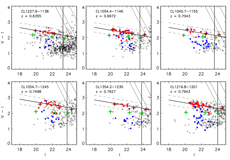
Figure 1: – continued

In Fig. 1 we show the colour-magnitude diagrams for the $18$ fields for which we have high quality spectroscopy. Clusters are shown in order of increasing redshift. Empty circles show objects for which our photometric redshift criterion gives a high probability of cluster membership (see Sec. 3.1). Red and blue filled circles represent spectroscopically confirmed members lacking/showing any emission line in their spectra respectively. We note that the typical detection limit for the [OII]3727 line is low in our spectra - approximately $2\,$Å (Poggianti et al., 2006). Thin slanted lines correspond to the $1$, $3$ and $5\sigma$ detection limits in the V-band, while the solid thick line in each panel represents the best fit to the colour–magnitude relation measured using a fixed slope of $-0.09$. The fit has been computed using the bi–weight estimator (Beers, Flynn & Gebhardt, 1990) on the objects without emission lines in their spectra (red filled circles). Dashed lines correspond to $\pm\,0.3$ mag from the best fit line.

Crosses in Fig. 1 show the location of galaxy models with two different star formation (SF) histories: a single burst at $z=3$ (dark red) and an exponentially declining SF starting at $z=3$ (green) with a characteristic time–scale ($\tau$) of $1$ Gyr. Both models were calculated using the population synthesis code by Bruzual & Charlot (2003) with a Chabrier initial mass function. For each SF history, three different metallicities are shown: $0.02$, $0.008$ and $0.004$, from brighter to fainter objects. The relation between metallicity and luminosity in these models has been calibrated by requiring that they reproduce the observed CMR in Coma (see Sec. 6). This calibration has been found a posteriori to be in good agreement with the metallicity–luminosity relation derived from spectral indices of Coma galaxies (Poggianti et al., 2001b). The solid vertical line in each panel of Fig. 1 shows the apparent magnitude which translates to M${}_{\rm V}=-18.2$ when evolved passively to $z=0$ using the single burst model. This magnitude limit was chosen so that all brighter objects are above the $5\sigma$ detection limit in the V–band in all of our clusters.

Note that the FORS2 field is $6\aas@@fstack{\prime}8\times 6\aas@@fstack{\prime}8$ with a pixel size of $0\aas@@fstack{\prime\prime}20$ and, after dithering, the field of view with the maximum depth of exposure is approximately $6.5^{\prime}\times 6.5^{\prime}$. For our infrared data, however, taking into account dithering and overlapping exposures, the field is $6.0^{\prime}\times 4.2^{\prime}$ for our intermediate redshift cluster candidates and $5.4^{\prime}\times 4.2^{\prime}$ for our high redshift cluster candidates. As explained in Sec. 3.1, galaxies likely to be cluster members are selected as having a probability within $\pm\,0.1$ of the cluster redshift above some threshold. Where there is no IR data, however, the redshift probability distributions are broader, and so cluster likelihoods are correspondingly lower and fewer galaxies meet the adopted criteria. While we have re–calibrated the photo-z cutoffs in the regions where no IR data are available so to use broader cuts in these regions, we have noted that some ‘edge effects’ remain. For these reasons, in this study we will only use the region for which we have both optical and infrared data for each of our fields.

The open circles shown in Fig. 1 correspond to objects within the fixed maximum physical radius centred on the BCG and included in the SOFI field. This physical radius turns out to be $\sim 0.74\,{\rm Mpc}$. For two of the fields shown in Fig. 1 (cl$1227.9$-$1138$ and cl$1103.7$-$1245$a), the BCG lies close to the edge of the chip (see Fig. 1 in Poggianti et al. 2006 and Fig. 6 in White et al. 2005). In these cases, the open circles show all the objects with high probability of cluster membership within the whole region for which we have infrared data.

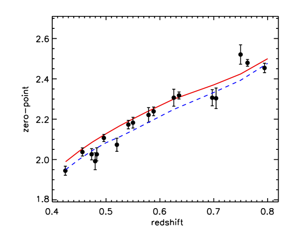
Figure 2: Evolution of the zero-point of the colour–magnitude relation as a function of redshift. Filled circles with error bars represent the values measured by fitting the observed relation. The solid and dashed lines show the predictions of a single burst model with formation redshift $3$ and $2$ respectively. In both cases, the zero-point has been measured at the apparent magnitude that corresponds to $M_{\rm V}=-20.$ when evolved to $z=0$.

Fig. 1 shows several interesting results. The single burst model seems to provide a good fit to the observed red sequence over all the redshift range sampled by the clusters under investigation. This confirms that the location of the CMR observed in distant clusters, requires high redshifts of formation, and that the slope is consistent with a correlation between galaxy metal content and luminosity. In Fig. 2, we show the evolution of the zero-point of the colour–magnitude relation as predicted by adopting the single burst model with formation redshift $3$ (solid line), and the values measured by fitting the observed relation for all the clusters in our sample (filled symbols with error bars). Both for the observational data and for the model predictions, the zero-point has been measured at the apparent magnitude that corresponds to $M_{\rm V}=-20$ when evolved to $z=0$. As mentioned before, the fit has been obtained using only the spectroscopically confirmed members without emission lines in their spectra (red filled circles in Fig. 1) and assuming a fixed slope of $-0.09$. Error bars have been estimated via bootstrap resampling of the galaxies used to compute the fit. Overall, the measured values follow nicely the model line, although some deviations are visible where the models are systematically redder than the best fit relations (see also Fig.1). These could indicate a lower formation redshift for red–sequence galaxies in these clusters. For a single burst model with formation redshift $2$, the predicted zero-point is lower at all redshifts, as indicated by the dashed line in Fig. 2. Within the errors, however, both single burst models provide a relatively good fit over all the redshift range under investigation.

Another interesting result shown in Fig. 1 was already noted in White et al. (2005): our sample shows large variations in the relative proportions of red and blue galaxies. Some clusters exhibit a strong red sequence with rather few blue galaxies (e.g. cl$1232.5$-$1250$, cl$1138.2$-$1133$) while others show many blue galaxies but relatively few passively evolving systems (e.g. cl$1040.7$-$1155$, cl$1227.9$-$1138$). So although the locus of red galaxies is well described by a uniformly old stellar population, the “morphology” of the colour–magnitude diagrams is quite varied. This must be related, at some level, to the dynamical and accretion histories of the clusters.

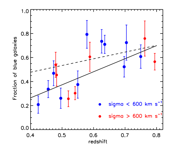
Figure 3: Fraction of galaxies bluer than $0.3$ mag from the best fit colour magnitude relation as a function of redshift. Red and blue symbols are for galaxy clusters with velocity dispersion larger and smaller than $600\,{\rm km}\,{\rm s}^{-1}$ respectively. Errors have been estimated using Poisson statistics. The solid and dashed line show linear fits to the data obtained by selecting cluster members using their photometric redshifts and statistical subtraction respectively. Points are shown for the former selection criterion. (See text for details).

In Fig. 3 we show the fraction of blue galaxies for the $18$ EDisCS fields shown in Fig. 1 as a function of redshift. Red and blue symbols are for clusters with velocity dispersion larger and smaller than $600\,{\rm km}\,{\rm s}^{-1}$ respectively. The blue fractions shown in Fig. 3 have been computed by counting the galaxies bluer than $0.3$ from the best fit colour–magnitude relation, and brighter than the passive evolution corrected limit that corresponds to $-18.2$ in the rest-frame V-band at $z=0$. All the objects which have a high probability of cluster-membership and within the same areas used for Fig. 1 are used. The solid line shows a linear fit to the data, while the dashed line shows a linear fit to data obtained using a statistical subtraction technique to determine cluster membership. Errors have been estimated using Poisson statistics. Our definition of blue fraction differs from the original definition introduced by Butcher & Oemler (1984). It is, however, interesting to note that results shown in Fig. 3 exhibit - as found for the first time by Butcher & Oemler (1984) - an increase in the fraction of blue galaxies with increasing redshift. The trend is present, although weaker, also when a statistical field subtraction instead of photometric redshift information is used to determine cluster membership. A Spearman’s rank correlation test gives a coefficient of $0.50$ with a significance level of $0.036$ in the case membership is defined using statistical subtraction, while in the case membership is defined using photometric redshifts, the coefficient is $0.69$ with a significance level of $0.001$. It should be noted, however, that the error bars are quite large and that there are large cluster-to-cluster variations at any given redshift.

We note that the constraints on the photometric redshift for blue galaxies are usually worse than those for galaxies of the same magnitude but with a redder colour, because of their smoother spectral energy distribution. The statistical subtraction technique is also more uncertain for blue galaxies because the field population that is used to perform the subtraction has a colour distribution peaked towards blue colours. In the following sections, we will concentrate on the distribution of galaxies along the red–sequence, where both the photometric redshift and the statistical subtraction method are expected to perform better.

5 The red–sequence galaxy distribution

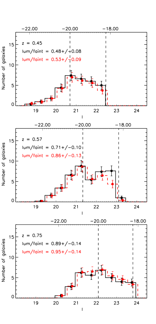
Figure 4: Number of galaxies along the red–sequence. Histograms have been obtained by stacking individual clusters in three redshift bins. Black and red histograms correspond to cluster membership based on photometric redshift and on statistical subtraction respectively. The scale on the top of each panel shows the rest–frame V–band magnitude that corresponds to the I–band magnitude and has been passively evolved to $z=0$. Vertical dashed lines show our magnitude limit and the edge between ‘luminous’ and ‘faint’ galaxies. A small offset has been added between two histograms in each panel for clarity. For each histogram, we give the luminous–to–faint ratio as defined in the text.

In De Lucia et al. (2004), we analysed the distribution of galaxies along the colour–magnitude relation for four of the highest redshift clusters in the EDisCS sample. As mentioned in Sec. 1, our analysis pointed out a significant deficit of faint red galaxies compared to the nearby Coma cluster. We interpreted this deficit as evidence for a large number of galaxies having moved onto the red–sequence relatively recently, possibly as a consequence of the suppression of their star formation by the dense cluster environment. If the scenario we envisaged is correct, then we should be able to see some evolution in the relative number of ‘faint’ and ‘luminous’ red galaxies as a function of redshift within our EDisCS sample.

In Fig. 4 we show the number of galaxies along the red–sequence obtained by averaging the distributions of individual clusters in three redshift bins. Black histograms are obtained by selecting all the galaxies for which our photometric redshift criterion gives a high probability of cluster membership (Sec. 3.1). Red histograms are obtained by selecting cluster members using a purely statistical subtraction (Sec. 3.2). In the latter case, we have averaged over $100$ Monte Carlo realizations of the statistical subtraction for each cluster. For the histograms shown in Fig. 4, all the ‘members’ within $\sim 0.5\times{\rm R}_{200}$ and within $\pm\,0.3$ mag of the best fit relation are used. In the present analysis, we are neglecting the clusters cl$1227.9$-$1138$ and cl$1103.7$-$1245$a for which the BCG lies at the edge of the chip. Furthermore, we also neglect the cluster cl$1119.3$-$1129$ which, as explained in White et al. (2005), shows a very weak concentration of galaxies close to the selected BCG and has a small value of ${\rm R}_{200}$. As a consequence, there are just a handful of galaxies on the red sequence within the fraction of virial radius we have adopted. In addition, we do not have infrared data for this cluster.

Clusters have been combined in three redshift bins (we end up with $5$ clusters in each bin) correcting colours and magnitudes to the central redshift of the corresponding bin. Corrections are based on the single burst model shown in Fig. 1 (results do not appreciably change using a single burst model with formation redshift $2$ instead of $3$). The scale on the top of each panel in Fig. 4 shows the rest–frame V–band magnitude corresponding to the observed I–band magnitude after correcting for passive evolution between the redshift of the bin and $z=0$.

As in De Lucia et al. (2004), we compute for each redshift bin a ‘luminous–to–faint’ ratio. We classify as ‘luminous’ all galaxies brighter than $M_{\rm V}=-20.0$ and as ‘faint’ those galaxies that are fainter than this magnitude and brighter than $M_{\rm V}=-18.2$. As mentioned in the previous section, the faint limit has been chosen because it corresponds to the limiting magnitude in the I–band for which all selected objects are above the $5\sigma$ detection limit in the V–band. As for the choice of the magnitude corresponding to the edge between faint and luminous galaxies, we use $-20$ because, at our highest redshift, it approximately equally divides the range of cluster galaxy magnitudes covered down to $-18.2$. Both limits correspond to values after passive evolution to $z=0$ and are indicated by vertical dashed lines in Fig. 4.

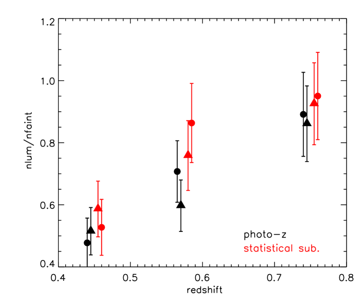
Figure 5: Luminous–to–faint ratio as a function of redshift. Circles and triangles are used in the case where all galaxies within $\sim 0.5\times{\rm R}_{200}$ or within $\sim 0.74\,{\rm Mpc}$ from the BCG are selected. Black and red symbols correspond to cluster membership based on photometric redshift and on statistical subtraction. Symbols corresponding to the same redshift have been displaced for clarity.

The values of the luminous–to–faint ratios computed for the histograms shown in Fig. 4 are listed in each panel, along with the estimated errors. Fig. 5 shows these values as a function of redshift. The error bars have been estimated assuming Poisson statistics and, in the case where cluster members are selected using a statistical subtraction, they include the error contribution from the background field (this is however negligible given the large area used for the subtraction). Circles in Fig. 5 correspond to the histograms plotted in Fig. 4, where all the cluster members within $\sim 0.5\times{\rm R}_{200}$ have been used. Triangles are used in the case where all the cluster members within a fixed physical distance ($\sim 0.74\,{\rm Mpc}$) from the BCG are retained. Red and black symbols correspond to membership criteria based on statistical subtraction and on photometric redshifts respectively.

The error bars shown in Fig. 5 are large, and some small differences arise from the use of different criteria for cluster membership and from different choices about the area used for the analysis. Overall, however, independently of the method employed and the area used, the data indicate a decrease of the luminous–to–faint ratio with decreasing redshift. Faint red galaxies become increasingly important with decreasing redshift or, in other words, the faint end of the colour–magnitude relation becomes increasingly populated with decreasing redshift. As noted in our previous paper, this finding is inconsistent with a formation scenario in which all red galaxies in clusters today evolved passively after a synchronous short duration event at $z\gtrsim 2-3$, and suggests that present day passive galaxies follow different evolutionary paths, depending on their luminosity.

It is now interesting to ask if this evolution in the luminous–to–faint ratio depends on cluster properties, for example mass or velocity dispersion. In Fig. 6 we again show the distribution of galaxies along the red–sequence. This time, we have combined the clusters in two redshift bins and, in each redshift bin, we have split the clusters according to their velocity dispersions. Red and blue histograms are for clusters with velocity dispersions larger and smaller than $600\,{\rm km}\,{\rm s}^{-1}$ respectively. Black histograms are obtained by stacking all the clusters in each redshift bin. Left panels are for the case where membership is based on photometric redshifts, while for the histograms shown on the right, membership is based on a purely statistical subtraction. All cluster members within $\sim 0.5\times{\rm R}_{200}$ from the BCG are used. In the lower redshift bin, we have $5$ clusters in each bin of velocity dispersion while in the higher redshift bin we have $2$ and $3$ clusters in the larger and smaller velocity dispersion bin respectively. The behaviour shown in Fig. 6 is not significantly different if all galaxies within a fixed physical radius from the BCG are used (see also Fig. 5).

The values listed in Fig. 6 show the same trend of an increasing luminous–to–faint ratio as a function of redshift and also hint at a dependence on cluster velocity dispersion. Clusters with large velocity dispersion seem to have a larger fraction of luminous galaxies with respect to the systems with smaller velocity dispersion. For the highest redshift bin, the difference goes in the same direction but is not statistically significant. The number statistics are, however, poor and the error bars are large so that it is difficult to draw any definitive conclusions. We find, however, similar results if we split the clusters on the basis of a richness estimate similar to that used in White et al. (2005), i.e. based on the number of red–sequence galaxies.

In a recent study, Tanaka et al. (2005) have investigated the build up of the colour–magnitude relation using deep panoramic imaging of two clusters at $z=0.83$ and $z=0.55$ respectively. Using photometric redshifts and statistical subtraction, and using nearest–neighbour density to characterise the environment, these authors conclude that build-up of the colour–magnitude relation is “delayed” in lower density environments. This is in apparent contradiction with our findings, although a direct comparison is not straightforward as we use the cluster velocity dispersion and not local density to differentiate environments. In addition, the conclusions of Tanaka et al. (2005) are based only on two clusters and these authors argue that their intermediate redshift cluster is “peculiar”. Finally, one should keep in mind that cluster–to–cluster variations are rather large (see Fig. 1). Further studies are therefore needed to confirm or disprove the apparent trends.

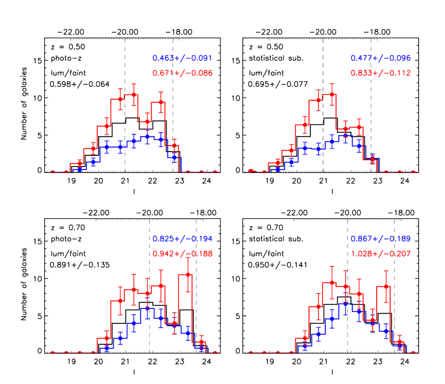
Figure 6: As in Fig. 4 for two redshift bins. Red and blue histograms are for clusters with velocity dispersion larger and smaller than $600\,{\rm km}\,{\rm s}^{-1}$ respectively. Black histograms are obtained by stacking all the clusters in each redshift bin. Left and right panels correspond to membership based on photometric redshifts and on statistical subtraction respectively. All cluster members within $\sim 0.5\times{\rm R}_{200}$ are used. Histograms in each panel have been slightly offset for clarity. The luminous–to–faint ratio (with the corresponding errors) are listed in each panel.

6 The red–sequence galaxy distribution in nearby clusters

In the previous section, we have analysed the evolution of the luminous–to–faint ratio over the redshift range sampled by our EDisCS clusters. We want now to set the zero–point for this evolution by studying the distribution of galaxies along the red–sequence in nearby galaxy clusters. In order to carry out a comparative study with the clusters in the EDisCS sample, we need relatively deep photometry (down to $-18.2$ in the rest–frame V–band) sampling the rest–frame U and V bands, and with good spatial coverage (at least $\sim 0.5\times{\rm R}_{200}$). These conditions are met by only a few nearby clusters. In the following we will describe in more detail the data and the analysis performed on our low redshift comparison sample, which is constituted by Coma, and a sample of clusters selected from the Sloan Digital Sky Survey (SDSS).

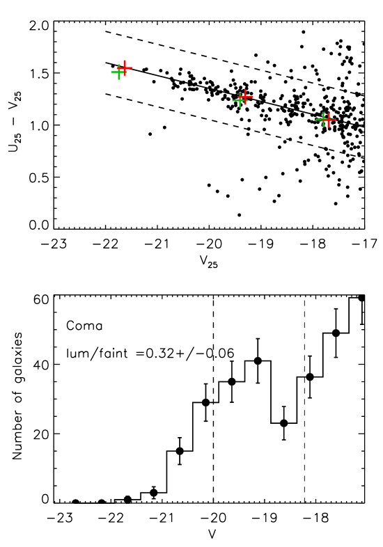
Figure 7: Colour–magnitude relation (top panel) and distribution of galaxies along the red–sequence (bottom panel) for the Coma cluster. The solid line in the top panel shows the best fit relation to the red–sequence. Crosses correspond to the same SF models shown in Fig. 1.

To date, Coma (A1656) remains the only rich cluster in the nearby Universe ($z=0.023$) with a high precision near–UV colour–magnitude relation, determined using hundreds of spectroscopically confirmed members. In this work, we have used magnitudes and colours in a $25\aas@@fstack{\prime\prime}2$ diameter aperture from Terlevich, Caldwell & Bower (2001). At the redshift of Coma, this corresponds to a physical size of $11.71$ kpc, quite closely approximating our $\sim 11$–$15$ kpc aperture from $z\sim 0.4$–$0.8$ (see Sec. 4). Observed magnitudes are converted to absolute magnitudes using the distance modulus of Coma computed using its redshift and the adopted cosmology ($35.00$). Observed colours are converted to rest–frame colours using tabulated K–corrections (Poggianti, 1997). The colour–magnitude relation of the Coma cluster, based on the catalogue by Terlevich et al. (2001), is plotted in the top panel of Fig. 7. The solid thick line shows the best fit relation determined using the bi–weight estimator, as for the EDisCS clusters. Dashed lines correspond to $\pm\,0.3$ mag from the best fit line. Crosses show predictions from the same two models shown in Fig. 1. We recall that the relation between metallicity and luminosity in these models has been calibrated by requiring that they reproduce the observed CMR in Coma.

The bottom panel of Fig. 7 shows the distribution along the red–sequence for this cluster. Membership information has been obtained using a redshift catalogue kindly provided by Matthew Colless and a procedure similar to that employed in Mobasher et al. (2003). Briefly, for each magnitude bin, we count how many objects have a measured spectroscopic redshift ($N_{z}$), and how many are spectroscopically confirmed members ($N_{c}$). We assume then that the spectroscopic sample is ‘representative’, i.e. that the fraction of galaxies that are cluster members is the same in the spectroscopic sample (that is incomplete) as in the photometric sample (that is complete). Cluster membership can then be obtained as the ratio between the two numbers computed before ($N_{c}/N_{z}$). The counts shown in the bottom panel of Fig. 7 are obtained correcting the raw distribution by this membership factor. The luminous–to–faint ratio we measure for Coma is $0.32\,\pm\,0.06$.

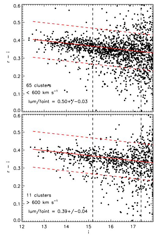
Figure 8: Stacked colour–magnitude relation for galaxy clusters selected from the C4 catalogue with velocity dispersion smaller (top panel) and larger than $600\,{\rm km}\,{\rm s}^{-1}$. The solid line in each panel shows the colour–magnitude relation predicted by a single burst model with formation redshift $3$. Dashed lines are offset from the solid line by $\pm\,0.1$. The vertical dashed lines correspond to ${\rm M}_{\rm V}=-20.18$ and ${\rm M}_{\rm V}=-18.25$ respectively. (See text for details).

We have complemented our low redshift comparison sample with a sample of clusters selected from the SDSS. The basis for the cluster sample used here is the C4 cluster catalogue by Miller et al. (2005). This catalogue is available for the SDSS Data Release $3$ and is based on the spectroscopic sample. The cluster detection algorithm employed for the construction of the C4 catalogue, is essentially based on an identification in a three-dimensional space (position, redshift, and colour). We refer to the original paper for more details. Based on the cluster redshifts and velocity dispersions given in the C4 catalogue, we have re-identified the BCG and measured the velocity dispersion at the virial radius for each cluster. Details about the procedure are described in von der Linden et al. (in preparation). For the purposes of this analysis, we have used the $76$ clusters below $z=0.045$ so to assure completeness down to the magnitude limit used for our analysis.

A direct comparison with the analysis of the red–sequence galaxies distribution performed above for the EDisCS clusters and for Coma is not simple, and requires a number of steps that we describe in the following. The first difficulty comes from the fact that, for the SDSS clusters, we have AB Petrosian magnitudes, while for the EDisCS clusters and for Coma we have used aperture magnitudes. In order to have an estimate of the correction necessary to convert Petrosian magnitudes into aperture magnitudes, we have compared our I–band aperture magnitudes to the ‘total’ magnitudes we used in White et al. (2005). We recall that an approximate total I-magnitude for each galaxy was estimated by adding to the Kron magnitude the correction appropriate for a point source measured within an aperture equal to the galaxy’s Kron aperture (we refer to the original paper for details). Using the median value of this correction, and considering that for elliptical like objects Petrosian magnitudes take into account about $80$ per cent of the light, we estimate that our aperture magnitudes can be converted into Petrosian magnitudes by a shift that varies between $-0.05$ and $-0.18$ from fainter to brighter galaxies.

In practice, we have converted the limits used before (${\rm M}_{\rm V}=-18.2$ and ${\rm M}_{\rm V}=-20$) into “Petrosian limits” (${\rm M}_{\rm V}=-18.25$ and ${\rm M}_{\rm V}=-20.18$). The conversion from apparent magnitudes to absolute magnitudes in the V–band has been performed using the routine KCORRECT by Blanton et al. (2003). For each cluster we have then constructed photometric catalogues by taking all the objects that are classified as galaxies by the SDSS pipeline and that reside within $\sim 0.5\times{\rm R}_{200}$ from the BCG. A corresponding field catalogue has been constructed by using the whole DR$3$ and for each cluster we have performed $50$ Monte Carlo realizations of the statistical subtraction procedure described in Sec. 3.2.

Fig. 8 shows, for one realization of the statistical subtraction, the stacked colour–magnitude diagrams for the two velocity dispersion bins. The solid line in each panel shows the relation predicted by a single burst model with formation redshift $3$, while dashed lines are offset from this line by $\pm 0.1$ mag. The vertical dashed lines show the limits used to define the luminous and faint population. We note that the magnitudes and colours plotted in Fig. 8 are given in the AB system. We have therefore used AB magnitudes and colours for the single burst model. The luminous–to–faint ratio computed from these stacked colour–magnitude relations are listed in each panel and are $0.39\pm 0.04$ for the high velocity dispersion bin, and $0.50\pm 0.03$ for the low velocity dispersion bin. The value measured for the clusters with velocity dispersion larger than $600\,{\rm km}\,{\rm s}^{-1}$ appears then compatible, within the errors, with that measured for the Coma cluster, while the value measured for clusters with lower velocity dispersion is significantly higher. We note also that the trend found for the SDSS clusters is the opposite of what we have found for our high redshift sample.

7 The buildup of the colour–magnitude relation

The results of our analysis are summarised in Fig. 9. Filled black circles show the values of the luminous–to–faint ratio for EDisCS clusters in three redshift bins. The values shown in Fig. 5, obtained for different choices of cluster membership criterion and area, have been averaged together. The error bars corresponding to these points have also been averaged, rather than combined in quadrature, in order to give a ‘conservative’ measure for the uncertainties. The green diamond shows the corresponding value for Coma. The orange and cyan triangles show the value measured for clusters selected from the SDSS with velocity dispersion larger and smaller than $600\,{\rm km}\,{\rm s}^{-1}$ respectively.

In De Lucia et al. (2004), we interpreted the deficit of faint galaxies found in the high redshift EDisCS clusters, as evidence that a large fraction of present–day passive faint galaxies must have moved onto the colour–magnitude relation at redshift lower than $0.8$. We argued that the population of blue galaxies observed in distant galaxy clusters provide the logical progenitors of faint red galaxies at $z=0$. It is therefore interesting to ask if the measured evolution in the luminous–to–faint ratio can be reproduced by simple evolution of the combined blue and red galaxies that populate the colour–magnitude diagrams of our high redshift clusters. In order to have a handle on this question, we have used the population synthesis model by Bruzual & Charlot (2003) to construct different exponentially declining star formation histories with $\tau=1,2,3$, and $7$ Gyr and a redshift of formation $3$. The same metallicities and normalisations used for the models shown in Fig. 1 have been adopted here. We have then started from the distribution of galaxies on the colour–magnitude diagram of the clusters in the highest redshift bin shown in Fig. 9 - for simplicity, we have used membership based on photometric redshift and a fixed physical distance from the BCG. For each galaxy bluer than $0.3$ mag than the best fit relation, we have determined the “closest model” in colour-magnitude space among those listed above. Each galaxy is then evolved to the next redshift bin by the amount predicted by the best fit model with the corresponding star formation history truncated at the redshift of the observation of the cluster (truncation model) or $1\,{\rm Gyr}$ later (delayed model). For the red–sequence galaxies (those in the stripe used to compute the luminous–to–faint ratio), we have simply used the single burst model described in Sec. 4. Using the same method, we use the distribution of galaxies in the colour-magnitude diagram of all higher redshift clusters to predict the evolution to $z=0.45$ and to $z=0.025$.

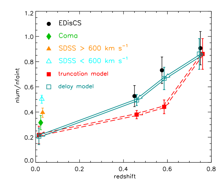
Figure 9: Luminous–to–faint ratio as a function of redshift. Filled circles show the average of the values shown in Fig. 5. The green diamond shows the values determined for Coma. The triangles show results for clusters selected from the SDSS with velocity dispersion larger (orange) and smaller (cyan) than $600\,{\rm km}\,{\rm s}^{-1}$. The arrows indicate the evolution of the luminous–to–faint ratio obtained using the models described in the text.

Model predictions are shown as red filled (truncation model) and open blue (delayed model) squares connected by arrows in Fig. 9. Interestingly, both models predict an amount of evolution from $z=0.75$ to $z\sim 0$ that is in nice agreement with that measured using the highest redshift EDisCS clusters and the Coma cluster. The predicted amount of evolution between $z\sim 0.4$ and $z\sim 0$ is instead too large to reproduce the luminous–to–faint ratios measured for the SDSS clusters. These appear to be compatible with the luminous–to–faint ratio measured for the EDisCS clusters at $z\sim 0.4$. In the truncation model, galaxies move onto the red–sequence very rapidly so that the predicted luminous–to–faint ratio lies below the measured value in the intermediate redshift bins. In the delayed model, galaxies stay blue longer so that the predicted evolution is closer to the observed trend at all redshifts sampled by the EDisCS clusters.

In Sec. 5 we have investigated how the distribution of galaxies on the red–sequence depends on the cluster velocity dispersion. The corresponding luminous–to–faint ratios (again averaged for different cluster membership criteria and different choices for the area) are shown in both panels of Fig. 10. Filled red and open blue circles are used for clusters with velocity dispersion larger and smaller than $600\,{\rm km}\,{\rm s}^{-1}$ respectively. The arrows connected by squares show the evolution predicted by the truncation (top panel) and delay (bottom panel) models described above. Triangles refer to the SDSS clusters as in Fig. 9. Both models predict a luminous–to–faint ratio that is close to observed value for low velocity dispersion clusters at redshift $z\sim 0.5$. For clusters with velocity dispersion larger than $600\,{\rm km}\,{\rm s}^{-1}$, both models instead predict a lower value than that measured for intermediate redshift EDisCS clusters. The values predicted for clusters with larger velocity dispersion are in both models and down to redshift zero, larger than the corresponding values for low velocity dispersion clusters. This appears in agreement with the trend found within our EDisCS, but in contradiction with that found for the SDSS clusters. In addition, as shown already in Fig. 9, the amount of evolution predicted between $z\sim 0.5$ and $z\sim 0$ is not compatible with the high luminous–to–faint ratios measured for the SDSS clusters.

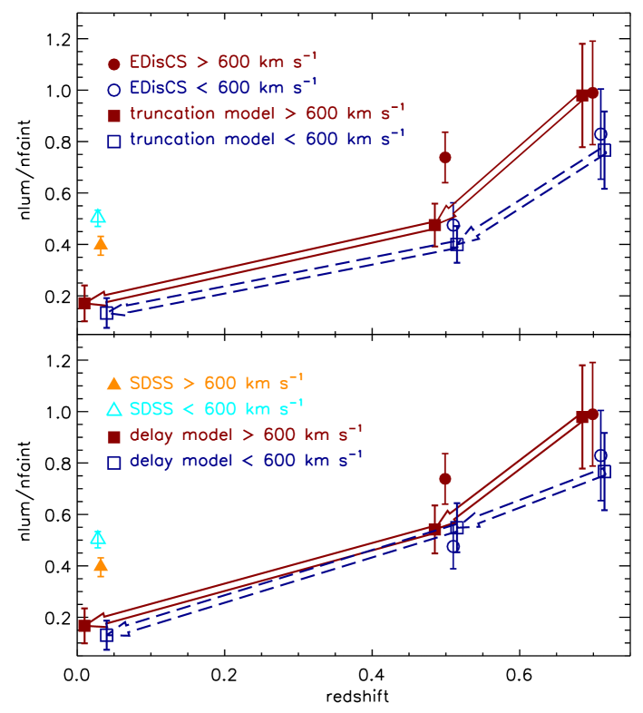
Figure 10: Luminous–to–faint ratio as a function of redshift for clusters split according to their velocity dispersions. Filled red and open blue circles are used for EDisCS clusters with velocity dispersions larger and smaller than $600\,{\rm km}\,{\rm s}^{-1}$ respectively. Triangles refer to the SDSS clusters as in Fig. 9. Squares connected by arrows show prediction from the truncation (top panel) and delay (bottom panel) described in the text.

We note that Table 4 in Poggianti et al. (2006) indicates that a cluster with velocity dispersion $\sim 600\,{\rm km}\,{\rm s}^{-1}$ at $z\sim 0.6$ evolves into a system with velocity dispersion $\sim 700\,{\rm km}\,{\rm s}^{-1}$ at $z\sim 0$. Therefore, it would be more correct to compare the values predicted from our models at $z\sim 0$ with those obtained for the SDSS by using a cut corresponding to $\sim 700\,{\rm km}\,{\rm s}^{-1}$. In this case, the measured luminous–to–faint ratios are $0.47\pm 0.03$ and $0.44\pm 0.06$ for the low and high velocity dispersion clusters respectively. The sample used in this study, however, only contains $4$ cluster with velocity dispersion larger than $\sim 700\,{\rm km}\,{\rm s}^{-1}$.

8 Discussion and conclusions

The tight colour–magnitude relation shown by cluster elliptical galaxies has been the subject of numerous studies that, in the last decade, have been pushed to higher and higher redshifts. An interesting and still controversial result of recent years is the claim of a ‘deficit’ of faint red galaxies at redshift $z\sim 1$. In our previous work (De Lucia et al., 2004), we analysed the distribution of galaxies on the red–sequence for four high redshift EDisCS clusters, and we compared such a distribution to that measured for the nearby Coma cluster. Although with a low significance level, we found that clusters at redshift $z\sim 0.8$ exhibit a ‘deficit’ of faint red sequence galaxies.

A decline in the number of red sequence members at faint magnitudes was first observed in clusters at $z=0.25$ by Smail et al. (1998). Evidence for a ‘truncation’ of the red–sequence was noted in an overdensity around a radio galaxy at $z=1.2$ by Kajisawa et al. (2000) and Nakata et al. (2001). The same authors, however, speculated that their result might be spurious because of limited area coverage ($<0.33$ Mpc) and strong luminosity segregation. (See also the discussion by Kodama et al. (2004) who obtain a similar result for early–type galaxies in a single deep field).

In recent work, Andreon (2006) has studied the red–sequence luminosity function for the cluster MS$1054$–$0321$. By comparing his result with the faint–end slope measured by fitting the red–sequence luminosity function of nearby clusters from the SDSS by Tanaka et al. (2005), he concluded that there is no evidence for a decreasing number of faint red galaxies at higher redshift. The results obtained by Andreon are based on a single cluster. The fitting procedure he adopted for the luminosity function of MS$1054$–$0321$ is not the same as that employed by Tanaka et al., and a comparison based on best fit parameters is plagued by the well known covariance between errors on ${\rm M}_{*}$ and on $\alpha$. In addition, we note that Tanaka et al. use an estimate of local density based on nearest–neighbour statistics. This complicates the comparison with MS$1054$–$0321$, a cluster with large velocity dispersion, bright X–ray luminosity and evident substructures (Donahue et al., 1998; Tran et al., 1999).

Evolution in the distribution of red–sequence galaxies is expected as a natural consequence of the recently established mass-dependence of elliptical galaxy evolution both in clusters and in the field (Thomas et al., 2005; Gallazzi et al., 2005; van der Wel et al., 2005; Treu et al., 2005; Holden et al., 2005; Nelan et al., 2005). The discussion above suggests the details are still uncertain. The error bars are large and large cluster–to–cluster variations preclude definitive conclusions. Nevertheless, the build–up of the colour–magnitude relation is of great interest, as it can constrain the relative importance of star formation and metallicity in establishing the observed properties of elliptical galaxies.

In this paper, we have used galaxy clusters from our EDisCS sample in order to extend our previous analysis to a wider redshift range and to study how this effect depends on cluster velocity dispersion. In agreement with previous work, we find that bright red–sequence galaxies in high redshift clusters can be described as an old, passively–evolving population. A single burst model with formation redshift of $3$, calibrated on the colour–magnitude relation of the nearby Coma cluster, provides a good fit to the red sequence observed over the full redshift range sampled by our clusters. This confirms earlier claims that the location of the red–sequence in distant clusters suggests high formation redshift, and that its slope is consistent with a correlation between metal content and luminosity.

However, within the same EDisCS sample, we also confirm our previous finding of a significant evolution in the luminosity distribution of red–sequence galaxies since $z\sim 0.8$. Combining clusters in three different redshift bins, and defining as ‘faint’ all galaxies in the passive evolution corrected range $0.4\,\gtrsim\,$L$/$L${}_{*}\,\gtrsim\,0.1$, we find a clear decrease in the luminous–to–faint ratio with decreasing redshift. The error bars and the cluster–to–cluster variation are large, but the measured trend is robust against variations in the criteria adopted for cluster membership and in the size of the region analysed. We have also investigated how this evolution depends on cluster velocity dispersion. At intermediate redshift, the luminous–to–faint ratio of clusters with velocity dispersion larger than $600\,{\rm km}\,{\rm s}^{-1}$ appears to be larger than that measured for clusters at the same redshift but with lower velocity dispersion. The error bars and the cluster–to–cluster variations are, however, too large to draw any definitive conclusions regarding this point.

Our low redshift comparison sample includes the Coma cluster, and a sample of clusters selected from the SDSS. For the Coma cluster, we find a value of the luminous–to–faint ratio that is significantly lower than the value obtained for the EDisCS clusters at $z\sim 0.45$. This is not the case for the luminous–to–faint ratios measured by stacking clusters from the SDSS in different velocity dispersion bins. These values are not significantly different from the values measured for the EDisCS clusters at $z\sim 0.45$.

Interestingly, we find the measured amount of evolution in the luminous–to–faint ratio from $z=0.75$ to $z\sim 0$ to be approximatively consistent with predictions of simple models where the blue bright galaxies that populate the colour–magnitude diagram of high redshift clusters, have their star formation truncated by the hostile cluster environment. Clearly the model we use is extremely simplified. We are assuming a single redshift of formation for all galaxies and guessing their star formation history simply on the basis of their location in the observed colour–magnitude diagram. In reality, galaxies will have a certain distribution of formation redshifts and this, together with age, metallicity and dust degeneracies, will certainly complicate the modelling. In addition, we are simply assuming that the star formation history is truncated at the cluster redshift (or 1 Gyr later) for all galaxies bluer than $0.3$ mag from the best fit red–sequence. Not all these galaxies are falling into the cluster at the time of our observations and the time–scale of the star formation suppression by the cluster environment (if there is a suppression of the star formation by the cluster environment) might be different than that assumed and/or depend on cluster or galaxy properties. Finally, we are neglecting further infall of galaxies between our various redshift bins. For all these reasons, our model results should be taken with caution. They simply suggest that a scenario in which infalling galaxies have their star formation histories truncated by the hostile cluster environment is in qualitative agreement with the observed build up of the colour–magnitude sequence. They do not yet convincingly confirm this scenario.

Our results indicate that present–day passive galaxies follow different evolutionary paths, depending on their luminosity (or mass). This conclusion is in line with recent results from fundamental–plane and stellar population studies (Thomas et al., 2005; van der Wel et al., 2005; Treu et al., 2005; Holden et al., 2005). More data are required to clarify if and how this depends on environment. Such studies will constrain the relative importance of star formation and metallicity in establishing the observed red–sequence, and thus clarify the physical mechanisms that drive the formation and evolution of the early type galaxy population in clusters.

References

- Andreon (2006) Andreon S., 2006, MNRAS, 369, 969
- Aragón-Salamanca et al. (1993) Aragón-Salamanca A., Ellis R. S., Couch W. J., Carter D., 1993, MNRAS, 262, 764
- Beers et al. (1990) Beers T. C., Flynn K., Gebhardt K., 1990, AJ, 100, 32
- Benítez (2000) Benítez N., 2000, ApJ, 536, 571
- Bertin & Arnouts (1996) Bertin E., Arnouts S., 1996, A&AS, 117, 393
- Blakeslee et al. (2003) Blakeslee J. P., Franx M., Postman M., Rosati P., Holden B. P., Illingworth G. D., Ford H. C., Cross N. J. G., et a., 2003, ApJ, 596, L143
- Blanton et al. (2003) Blanton M. R., Brinkmann J., Csabai I., Doi M., Eisenstein D., Fukugita M., Gunn J. E., Hogg D. W., Schlegel D. J., 2003, AJ, 125, 2348
- Bolzonella et al. (2000) Bolzonella M., Miralles J.-M., Pelló R., 2000, A&A, 363, 476
- Bower et al. (1998) Bower R. G., Kodama T., Terlevich A., 1998, MNRAS, 299, 1193
- Brunner & Lubin (2000) Brunner R. J., Lubin L. M., 2000, AJ, 120, 2851
- Bruzual & Charlot (2003) Bruzual G., Charlot S., 2003, MNRAS, 344, 1000
- Butcher & Oemler (1984) Butcher H., Oemler A., 1984, ApJ, 285, 426
- Cole et al. (2000) Cole S., Lacey C. G., Baugh C. M., Frenk C. S., 2000, MNRAS, 319, 168
- De Lucia & Blaizot (2006) De Lucia G., Blaizot J., 2006, astro-ph/0606519
- De Lucia et al. (2004) De Lucia G., Kauffmann G., White S. D. M., 2004, MNRAS, 349, 1101
- De Lucia et al. (2004) De Lucia G., Poggianti B. M., Aragón-Salamanca A., Clowe D., Halliday C., Jablonka P., Milvang-Jensen B., Pelló R., Poirier S., Rudnick G., Saglia R., Simard L., White S. D. M., 2004, ApJ, 610, L77
- De Lucia et al. (2006) De Lucia G., Springel V., White S. D. M., Croton D., Kauffmann G., 2006, MNRAS, 366, 499
- de Propris et al. (1998) de Propris R., Eisenhardt P. R., Stanford S. A., Dickinson M., 1998, ApJ, 503, L45
- de Vaucouleurs (1961) de Vaucouleurs G., 1961, ApJS, 5, 233
- Donahue et al. (1998) Donahue M., Voit G. M., Gioia I., Lupino G., Hughes J. P., Stocke J. T., 1998, ApJ, 502, 550
- Driver et al. (1998) Driver S. P., Couch W. J., Phillipps S., Smith R., 1998, MNRAS, 301, 357
- (22) Ferreras I., Charlot S., Silk K., 1999, ApJ, 521, 81 301, 357
- Finn et al. (2005) Finn R. A., Zaritsky D., McCarthy Jr. D. W., Poggianti B., Rudnick G., Halliday C., Milvang-Jensen B., Pelló R., Simard L., 2005, ApJ, 630, 206
- Firth et al. (2003) Firth A. E., Lahav O., Somerville R. S., 2003, MNRAS, 339, 1195
- Gallazzi et al. (2005) Gallazzi A., Charlot S., Brinchmann J., White S. D. M., Tremonti C. A., 2005, MNRAS, 362, 41
- Gladders et al. (1998) Gladders M. D., Lopez-Cruz O., Yee H. K. C., Kodama T., 1998, ApJ, 501, 571
- Gladders & Yee (2005) Gladders M. D., Yee H. K. C., 2005, ApJS, 157, 1
- Gonzalez et al. (2001) Gonzalez A. H., Zaritsky D., Dalcanton J. J., Nelson A., 2001, ApJS, 137, 117
- Halliday et al. (2004) Halliday C., Milvang-Jensen B., Poirier S., Poggianti B. M., Jablonka P., Aragón-Salamanca A., Saglia R. P., De Lucia G., Pelló R., Simard L., Clowe D. I., Rudnick G., Dalcanton J. J., White S. D. M., Zaritsky D., 2004, A&A, 427, 397
- Hatton et al. (2003) Hatton S., Devriendt J. E. G., Ninin S., Bouchet F. R., Guiderdoni B., Vibert D., 2003, MNRAS, 343, 75
- Holden et al. (2004) Holden B. P., Stanford S. A., Eisenhardt P., Dickinson M., 2004, AJ, 127, 2484
- Holden et al. (2005) Holden B. P., van der Wel A., Franx M., Illingworth G. D., Blakeslee J. P., van Dokkum P., Ford H., Magee D., Postman M., Rix H.-W., Rosati P., 2005, ApJ, 620, L83
- Johnson et al. (2006) Johnson O., Best P., Zaritsky D., Clowe D., Aragón-Salamanca A., Halliday C., Jablonka P., Milvang-Jensen B., Pelló R., Poggianti B. M., Rudnick G., Saglia R., Simard L., White S., 2006, MNRAS, 371, 1777
- Jørgensen et al. (2005) Jørgensen I., Bergmann M., Davies R., Barr J., Takamiya M., Crampton D., 2005, AJ, 129, 1249
- Kajisawa et al. (2000) Kajisawa M., Yamada T., Tanaka I., Maihara T., Iwamuro F., Terada H., Goto M., Motohara K., et a., 2000, PASJ, 52, 61
- Kauffmann & Charlot (1998) Kauffmann G., Charlot S., 1998, MNRAS, 294, 705
- Kodama et al. (1998) Kodama T., Arimoto N., Barger A. J., Aragón-Salamanca A., 1998, A&A, 334, 99
- Kodama & Bower (2001) Kodama T., Bower R. G., 2001, MNRAS, 321, 18
- Kodama et al. (2005) Kodama T., Tanaka M., Tamura T., Yahagi H., Nagashima M., Tanaka I., Arimoto N., Futamase T., et a., 2005, PASJ, 57, 309
- Kodama et al. (2004) Kodama T., Yamada T., Akiyama M., Aoki K., Doi M., Furusawa H., Fuse T., Imanishi M., et a., 2004, MNRAS, 350, 1005
- Larson (1974) Larson R. B., 1974, MNRAS, 169, 229
- McCracken et al. (2001) McCracken H. J., Le Fèvre O., Brodwin M., Foucaud S., Lilly S. J., Crampton D., Mellier Y., 2001, A&A, 376, 756
- Mei et al. (2006) Mei S., Blakeslee J. P., Stanford S. A., Holden B. P., Rosati P., Strazzullo V., Homeier N., Postman M., et a., 2006, ApJ, 639, 81
- Miller et al. (2005) Miller C. J., Nichol R. C., Reichart D., Wechsler R. H., Evrard A. E., Annis J., McKay T. A., Bahcall N. A., Bernardi M., Boehringer H., Connolly A. J., Goto T., Kniazev A., Lamb D., Postman M., Schneider D. P., Sheth R. K., Voges W., 2005, AJ, 130, 968
- Mobasher et al. (2003) Mobasher B., Colless M., Carter D., Poggianti B. M., Bridges T. J., Kranz K., Komiyama Y., Kashikawa N., Yagi M., Okamura S., 2003, ApJ, 587, 605
- Nakata et al. (2001) Nakata F., Kajisawa M., Yamada T., Kodama T., Shimasaku K., Tanaka I., Doi M., Furusawa H., et a., 2001, PASJ, 53, 1139
- Nelan et al. (2005) Nelan J. E., Smith R. J., Hudson M. J., Wegner G. A., Lucey J. R., Moore S. A. W., Quinney S. J., Suntzeff N. B., 2005, ApJ, 632, 137
- Pimbblet et al. (2002) Pimbblet K. A., Smail I., Kodama T., Couch W. J., Edge A. C., Zabludoff A. I., O’Hely E., 2002, MNRAS, 331, 333
- Poggianti (1997) Poggianti B. M., 1997, A&AS, 122, 399
- Poggianti et al. (2001a) Poggianti B. M., Bridges T. J., Carter D., Mobasher B., Doi M., Iye M., Kashikawa N., Komiyama Y., Okamura S., Sekiguchi M., Shimasaku K., Yagi M., Yasuda N., 2001a, ApJ, 563, 118
- Poggianti et al. (2001b) Poggianti B. M., Bridges T. J., Mobasher B., Carter D., Doi M., Iye M., Kashikawa N., Komiyama Y., Okamura S., Sekiguchi M., Shimasaku K., Yagi M., Yasuda N., 2001b, ApJ, 562, 689
- Poggianti et al. (2006) Poggianti B. M., von der Linden A., De Lucia G., Desai V., Simard L., Halliday C., Aragón-Salamanca A., Bower R., et a., 2006, ApJ, 642, 188
- Postman et al. (2005) Postman M., Franx M., Cross N. J. G., Holden B., Ford H. C., Illingworth G. D., Goto T., Demarco R., et a., 2005, ApJ, 623, 721
- Rudnick et al. (2001) Rudnick G., Franx M., Rix H.-W., Moorwood A., Kuijken K., van Starkenburg L., van der Werf P., Röttgering H., van Dokkum P., Labbé I., 2001, AJ, 122, 2205
- Schlegel et al. (1998) Schlegel D. J., Finkbeiner D. P., Davis M., 1998, ApJ, 500, 525
- Smail et al. (1998) Smail I., Edge A. C., Ellis R. S., Blandford R. D., 1998, MNRAS, 293, 124
- Springel et al. (2005) Springel V., White S. D. M., Jenkins A., Frenk C. S., Yoshida N., Gao L., Navarro J., Thacker R., Croton D., Helly J., Peacock J. A., Cole S., Thomas P., Couchman H., Evrard A., Colberg J., Pearce F., 2005, Nature, 435, 629
- Stanford et al. (2005) Stanford S. A., Eisenhardt P. R., Brodwin M., Gonzalez A. H., Stern D., Jannuzi B. T., Dey A., Brown M. J. I., McKenzie E., Elston R., 2005, ApJ, 634, L129
- Stanford et al. (1998) Stanford S. A., Eisenhardt P. R., Dickinson M., 1998, ApJ, 492, 461
- Strazzullo et al. (2006) Strazzullo V., Rosati P., Stanford S. A., Lidman C., Nonino M., Demarco R., Eisenhardt P. E., Ettori S., Mainieri V., Toft S., 2006, A&A, 450, 909
- Tanaka et al. (2005) Tanaka M., Kodama T., Arimoto N., Okamura S., Umetsu K., Shimasaku K., Tanaka I., Yamada T., 2005, MNRAS, 362, 268
- Terlevich et al. (2001) Terlevich A. I., Caldwell N., Bower R. G., 2001, MNRAS, 326, 1547
- Terlevich et al. (1999) Terlevich A. I., Kuntschner H., Bower R. G., Caldwell N., Sharples R. M., 1999, MNRAS, 310, 445
- Thomas et al. (2005) Thomas D., Maraston C., Bender R., de Oliveira C. M., 2005, ApJ, 621, 673
- Tran et al. (1999) Tran K.-V. H., Kelson D. D., van Dokkum P., Franx M., Illingworth G. D., Magee D., 1999, ApJ, 522, 39
- Treu et al. (2005) Treu T., Ellis R. S., Liao T. X., van Dokkum P. G., 2005, ApJ, 622, L5
- Valtchanov et al. (2004) Valtchanov I., Pierre M., Willis J., Dos Santos S., Jones L., Andreon S., Adami C., Altieri B., Bolzonella M., Bremer M., Duc P.-A., Gosset E., Jean C., Surdej J., 2004, A&A, 423, 75
- van der Wel et al. (2005) van der Wel A., Franx M., van Dokkum P. G., Rix H.-W., Illingworth G. D., Rosati P., 2005, ApJ, 631, 145
- Visvanathan & Sandage (1977) Visvanathan N., Sandage A., 1977, ApJ, 216, 214
- White et al. (2005) White S. D. M., Clowe D. I., Simard L., Rudnick G., De Lucia G., Aragón-Salamanca A., Bender R., Best P., et a., 2005, A&A, 444, 365
- Wilson et al. (2006) Wilson G., Muzzin A., Lacy M., Yee H., Surace J., Lonsdale C., Hoekstra H., Majumdar S., Gilbank D., Gladders M., 2006, preprint, astro-ph/0604289
- Zaritsky et al. (1997) Zaritsky D., Nelson A. E., Dalcanton J. J., Gonzalez A. H., 1997, ApJ, 480, L91