Unveiling the X-ray/TeV engine in Mkn 421

Abstract

Aims. Multi-wavelengths observations of TeV blazars provide important clues into particle acceleration in relativistic jets.

Methods. Simultaneous observations of Mkn 421 were taken in very high energy $\gamma$-rays ($>200\,\rm GeV$, CAT experiment), X-rays (RXTE) and optical (KVA). Multi-day RXTE observations are also presented, allowing for detailed modelling of the spectral variability.

Results. Short timescale ($\approx 30$ mn) variations in VHE $\gamma$-rays are found, correlated with X-rays but not with the optical. The X-ray spectrum hardens with flux until the photon indices saturate above a threshold flux $\approx 10^{-9}$erg s^-1 cm^-2. The fractional variability decreases from X-rays to optical as a power-law with $F_{\rm var}\propto E^{0.24\pm 0.01}$. The full spectral energy distribution is well-fitted by synchrotron self-Compton emission from cooling electrons injected with a Maxwellian distribution of characteristic energy $\gamma_{b}$. Fluctuations in the injected power with $P_{\rm inj}\propto\gamma_{b}^{4}$ explain the observed variability.

Conclusions. The spectral saturation and the power-law dependence of the fractional variability are novel results which may extend to other TeV blazars. The ability of Maxwellian injections to reproduce the observed features suggest second-order Fermi acceleration or magnetic reconnection may play the dominant role in particle acceleration.

1 Introduction

Mkn 421 was the first Active Galactic Nuclei (AGN) to be established as a TeV emitter (Punch et al. 1992). Such very high energy (VHE) $\gamma$-ray emission is thought to arise from particles accelerated in a relativistic jet directed along our line-of-sight. Continuous improvements in Atmospheric Cherenkov Telescopes (ACT) have resulted in new detections of sources, shedding new light on the underlying processes, notably in conjunction with X-ray observatories. Mkn 421, Mkn 501 and 1ES 1959$+$650 are the brightest VHE extragalactic objects detected so far, with VHE flares reaching levels many times that of the Crab flux (see e.g. Konopelko et al. 2003). Bright objects like these can be studied with ACTs on smaller time scales than fainter objects since there are more photons.

Variability in Mkn 421 is present at all wavelengths and correlations during high states have been found from millimeter wavelength observations up to VHE energies suggesting a single population of particles may be responsible, if only partly, for radiation over most of the spectrum. The flux doubling timescales vary widely but are correlated with energy as the highest energies vary faster.

The spectral energy distribution (SED) has the typical double-humped blazar feature in $\nu F_{\nu}$ representation, where the peaks are separated by 8 to 10 orders of magnitude in energy. The lower component is attributed to synchrotron radiation from relativistic electrons/positrons, and peaks at a frequency $\nu_{S}$ which ranges from $\approx$ 0.1 keV in a low activity state to a few keV in flaring cases, being clearly correlated with the intensity (Tanihata et al. 2004). The higher component can be interpreted as inverse Compton scattering of leptons on the synchrotron photons themselves. An alternative to leptonic models are the so-called ”hadronic models” where the relativistic jet has a significant component of relativistic protons emitting X-rays and $\gamma$-rays via synchrotron, photo-production, or pion decay from proton-proton interactions (see e.g. Costamante 2004 for a recent review).

Mkn 421 was in a historically high state in the first months of 2001, triggering a multi-wavelength campaign and spawning a wealth of observations with unprecedented detection levels in most energy bands. The campaign included amongst others the ground-based CAT Cherenkov telescope (200 GeV - 20 TeV), the RXTE X-ray observatory (2-30 keV) and the 60 cm KVA telescope on La Palma. The RXTE follow-up campaign was optimised for the Whipple ACT, but some observations occured during nights at the location of the CAT observatory. An analysis of the 4 ks segment that happened to exactly overlap with CAT and its impact on SED modeling, are discussed here. Multi-day spectral analysis of the X-ray data is also presented. Observations and analysis are found in §2, the results are collected in §3. A model of the SED is developped in §4 and the interpretation of the results is discussed in §5 before concluding.

2 Observations and data analysis

The data taking, reduction and analysis for CAT and RXTE is described next. The KVA telescope data shown in this paper have been presented by Sillanpää et al. (2001) where the reduction and analysis is described.

2.1 CAT

The CAT (Cherenkov Array at Thémis) imaging telescope operated on the site of the former solar plant Thémis in the French Pyrénées from 1996 to 2003. The detector collects Cherenkov light from the particles in atmospheric air-showers with a 17.8 ${\rm m}^{2}$ dish. The light is recorded by a high definition camera with a 4.8^∘ field-of-view, comprised of a central region of 546 phototudes in a hexagonal matrix spaced out by 0.13^∘ and of 54 surrounding tubes in two “guard rings”. A full description of the detector can be found in Barrau et al. (1998).

The observations were carried out on the night of 23-24 March 2001 when the source was very active in X-rays. The observations were made in the so-called wobble mode, i.e. the source position $\@vec{S}$ is shifted by 0.29^∘ from the field-of-view center. Showers pointing to this position are considered as ON-source data. Showers pointing to the symmetrical position $\@vec{S^{\prime}}$ with respect to the center are considered OFF data and have been used to monitor the cosmic-ray background.

The $\gamma$-ray image analysis, i.e. the method and the cuts, is based on the standard CAT procedure (Le Bohec et al. 1998). Individual events are compared to abacus of theoretical average images in order to derive the primary direction and the energy of events. The extraction of the $\gamma$-ray signal from the remaining background events is based on a novel statistical method using a maximum likelihood fit (Khélifi 2001). This method gives an estimation of the number of $\gamma$-rays, ${\rm N}_{\gamma,f}$, and of the source position, $\@vec{S}_{f}$ given the observational informations of each shower, the fitted arrival direction, $\@vec{D}$, the fitted shower impact parameter on the ground, $\@vec{IP}$ and the pointing elevation of the telescope, $\theta$. The likelihood function, $\mathcal{L}$, is defined by the product of the probability density of each event over all events passing cuts in the field of view (${\rm N}_{\rm TOT}$):

$$\mathcal{L}(\@vec{D}|{\rm N}_{\gamma,f},\@vec{S}_{f},\@vec{IP},\theta)=\prod_{i=1}^{{\rm N}_{\rm TOT}}p(\@vec{D}|{\rm N}_{\gamma,f},\@vec{S}_{f},\@vec{IP},\theta)$$

The probability density $p$ of each event can be separated as a function of the shower type, i.e. a $\gamma$-ray origin or an hadronic origin:

$$p={\rm N}_{\gamma,f}/{\rm N}_{\rm TOT}\times p_{\gamma}(\@vec{D}|\@vec{S}_{f},\@vec{IP},\theta)+$$

$$(1-{\rm N}_{\gamma,f}/{\rm N}_{\rm TOT})\times p_{h}(\@vec{D}|\@vec{IP},\theta)$$

The term $p_{\gamma}$ is the point spread function (PSF) of the CAT detector. It is determined from Monte-Carlo simulations of $\gamma$-rays with a power-law distribution in energy and for different bins in elevation angles. The exact value of the power-law index is not critical because the PSF extension is dominated by the lowest energy events. A differential spectrum $d{\rm N}/d{\rm E}\propto{\rm E}^{-2.7}$ was chosen. The term $p_{h}$ is the probability to reconstruct a shower arrival direction $\@vec{D}$ for a hadronic shower.

As the true arrival directions of hadronic events (cosmic rays) are isotropic, $p_{h}$ can be parameterized from data taken in fields of view without any known $\gamma$-ray source.

The likelihood $\mathcal{L}$ is maximised numerically according to the parameters ${\rm N}_{\gamma,f}$ and $\@vec{S}_{f}$. For the analysis of the Mkn 421 data, the source position $\@vec{S}_{f}$ has been fixed to the AGN position in order to achieve a better $\gamma$-ray extraction. This statistical method has been tested on simulations and on data taken on the Crab Nebula. No bias on the reconstructed number of $\gamma$-ray events is detectable, whatever the signal strength.

The significance of the signal is calculated from ratio of the maximum likelihood calculated on the data, $\mathcal{L}({\rm N}_{\gamma,f})$ to the likelihood calculated by assuming that no signal is present, $\mathcal{L}({\rm N}_{\gamma}=0)$. The exact formula of the significance estimation is:

$$\sigma=\sqrt{2\times\log{(\mathcal{L}({\rm N}_{\gamma,f})/\mathcal{L}({\rm\ N}_{\gamma}=0))}}$$

It has been checked on simulations that this significance estimation follows a Gaussian distribution of variance equal to 1 in absence of any signal.

The characteristics of the cuts described above and this statistical method for the signal extraction have been computed with a $\gamma$-ray spectrum of spectral index of $\Gamma$=2.55 ($d{\rm N}/d{\rm E}\propto{\rm E}^{-\Gamma}$), an integral flux comparable to the one of the Crab Nebula and at a telescope elevation of $\theta$=60^∘. About 41% of the $\gamma$-ray events are kept and the expected significance for 1 hour of observation is $5.7\,\sigma/\sqrt{\rm 1hour}$. This method gives better performances than a method based on a classical subtraction “ON-OFF” (e.g. Djannati-Atai et al. 1999).

The determination of the spectra and the integral fluxes are made with the standard CAT method (Piron et al. 2001). Briefly, the spectrum extraction is based on forward-folding method in which a parametrization of the spectrum shape is assumed. And the fluxes are calculated assuming a spectral shape derived by the previous method. In both determinations, the number of $\gamma$-ray events used for them is extracted by the maximum likelihood method described previously.

After selecting data based on clear weather conditions and stable detector operation, a total of 2.3 hours (corrected from dead time) of observations are kept, all taken within a elevation angle between 70^∘ and 90^∘. The number of $\gamma$-rays extracted by the maximum likelihood method are $1362\pm 50$ were detected. The flux was high enough to have significant data points with a 10 minute sampling. This lightcurve is represented in panel (a) of Figure 1. The integral flux is derived as a function of time assuming a non-evolving spectrum throughout the night (as it is justified by the study of the hardness ratio in the section 3.1). A flux decrease of 63% (significance of 2.3$\sigma$) within 30 min is followed by a doubling of the flux in 30 min again (significance of 3.8$\sigma$). These variability timescales had not been detected by CAT on Mkn 421 before these observations.

The VHE time scale variability of Mkn 421 has been addressed in past observations. The Whipple observatory’s 10 m telescope reported a $\gamma$-ray rate halving time scale of $\simeq 1\,{\rm h}$ on a flare in 1999 (Maraschi et al. 1999), but this has to be untangled from effective area effects before it can be assumed that the variability is intrinsic. The fastest doubling time scale reported by Whipple was 15 min (Gaidos et al. 1996), also expressed in rate rather than flux, though it can probably be assumed that effective areas do not double on this timescale. No reference could be found from Whipple where the lightcurve is expressed in integrated flux. The HEGRA collaboration observed the same flaring period but due to poor weather could not report on this specific episode. A lightcurve derived in units of integrated flux above 1 TeV shows a halving timescale of $\leq 1\,{\rm h}$ for the night of MJD 51939/40 (Aharonian et al. 2003). The halving timescale reported here is therefore consistent with other ACT measurements, but it is the fastest variability seen in an effective area independent way.

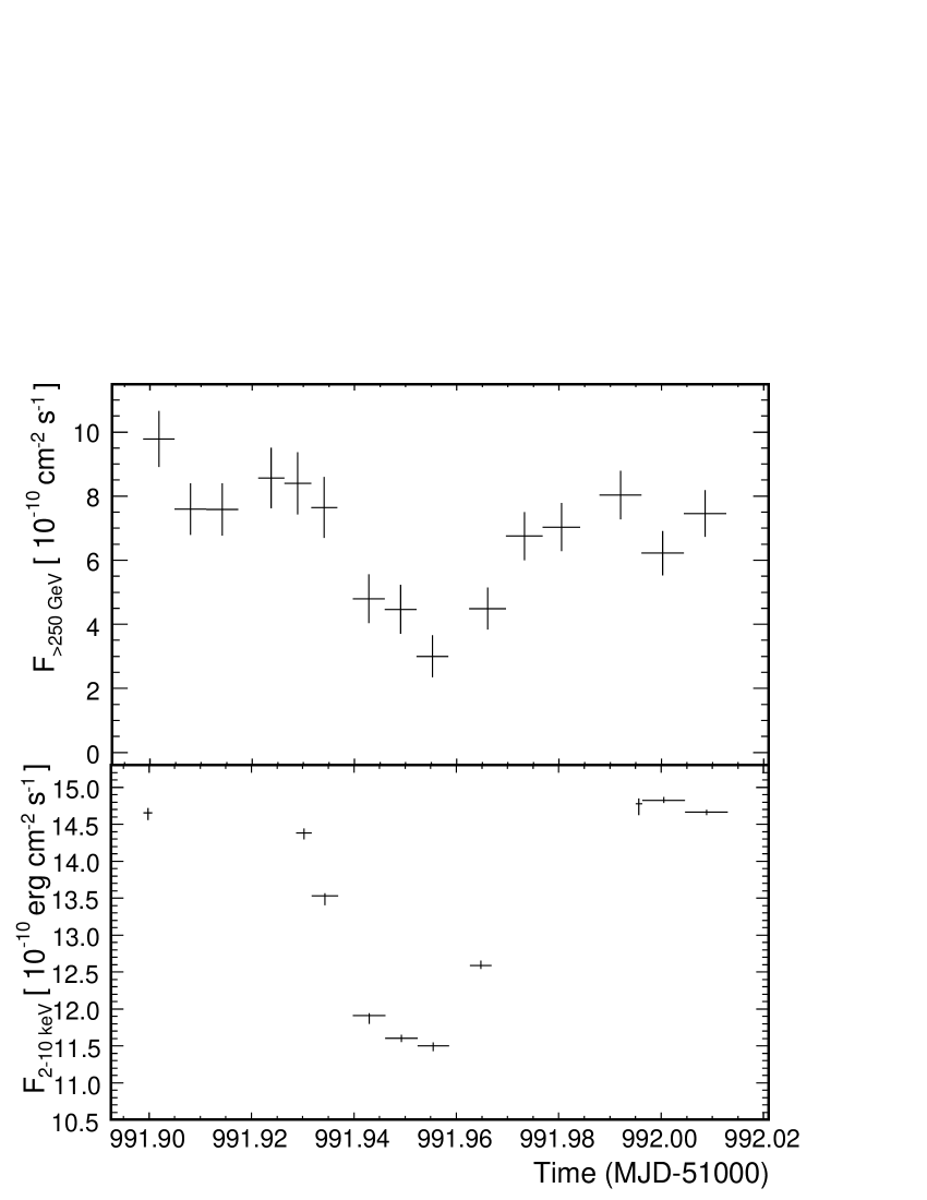
Figure 1: Top: CAT lightcurve on the night of 23 March 2001 expressed as integrated flux above $200\,\rm{GeV}$. The flux decreases by a factor $\geq 2$ within 30 min which is the fastest variability seen on Mkn 421 by CAT. Bottom: RXTE 2-10 keV flux lightcurve for observation times exactly overlapping or contained within a CAT measurement. The variability in the VHE band is larger than in the X–rays.

2.2 RXTE

The X–ray data set used here is publicly available , covering an outburst in Mkn 421 between MJD 51986 and MJD 51994 (the whole ObsID has a set of smaller observations that extend until MJD 52000 but were not included here). The source was detected with a rate that required the bright background model. The high rate allows to segment the data into segments of a few $100\,{\rm s}$ from which a spectrum and lightcurve expressed in ${\rm erg}\,{\rm cm}^{-2}\,{\rm s}^{-1}$ can be derived instead of the usual counting rate. Hence, the correlation between flux and spectral indices can be studied on the same time scales instead of using rate vs hardness ratios. This can be particularly relevant if, such as the case here, the spectrum changes significantly when the brightness changes.

A small part of the Mkn 421 observation campaign of RXTE is simultaneous with CAT, corresponding to observations taken between MJD 50991.8 and MJD 50992.1. This segment is analysed such that the RXTE data segments are made to match the CAT time segments. This means that the X-ray spectral file from which the flux is derived is at most as long as the CAT segments from which a flux, hardness ratio or spectrum was derived, the latter being just one big segment lasting the whole observation night of 24 March 2001.

The reduction scheme for the X-ray data set is the following:

• The STANDARD2 data are extracted in GOODTIME intervals constrained to be either a segment at most 400 s long, or at most as long as the overlapping length of a VHE observation by CAT, or at most as long as the whole CAT data set used to derive the VHE spectrum. Due to the variable active PCU configuration during these observations, this is done for each PCU independently.

• The PCU dependent PHA files are combined using the addspec tool weighted by the counts information delivered by fstatistic and then the corresponding response matrices were combined with addrmf. The bright background model was used and only the 3–40 PHA channel range was kept in XSPEC v. 12.2, or approximately 2–$20\,\rm keV$.

• These segments are then fitted to a power-law and a broken power-law in XSPEC with PCU configuration-dependent response matrices generated by the ftool pcarsp v. 10.1 and a fixed column density of $N_{\rm H}=1.6\times 10^{20}$ cm^-2 obtained from PIMMS. The chisquare probability $P(\chi^{2})$ for both models is estimated. For the time averaged spectrum, a double broken power-law is used.

  

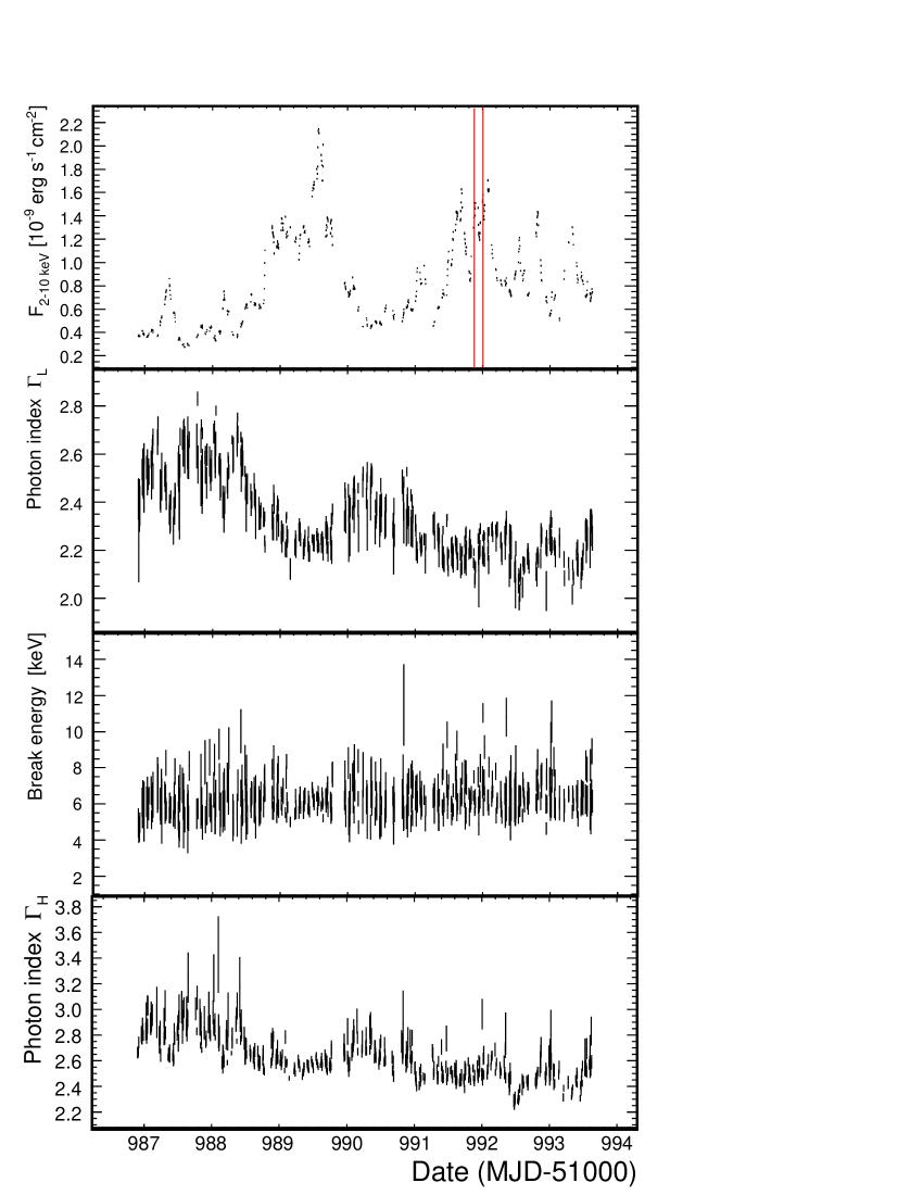
  Figure 2: Parameters derived from the broken power-law fits to the observation segments, as a function of MJD. The lines in the upper panel indicate the segment where simultaneous observations were possible with CAT. Whereas there is a clear indication of modulation and a flux dependency of both $\Gamma_{\rm L}$ and $\Gamma_{\rm H}$, no such indication is visible for the break energy.

• This yields the flux and the error (defined here as the 1-sigma confidence level) on the flux reported in the lightcurve, in units of $10^{-11}$ erg s^-1 cm^-2 in the 2-10 keV band, as well as spectral parameters for each of these intervals, namely the lower photon index $\Gamma_{\rm L}$, the break energy $E_{\rm br}$ and the upper photon index $\Gamma_{\rm H}$. The broken power-law fit yielded better fit results than a single power-law in 97% of the fits. If the single power-law is preferred with a higher $P(\chi^{2})$ then both indices are set to the single power-law value. Since the data segments do not have similar lenghts, the error on the flux can vary but is correlated with the integration time (shorter segments have an higher associated flux error). A small amount of segments had integration times $<200\,{\rm s}$ and were discarded from the analysis to keep those with a meaningful statistical error.

The lightcurve derived to match the CAT lightcurve is represented in panel (b) of Figure 1. The total lightcurve for the analysed proposal 60145 is in panel (a) of Figure 2 along with the curve indicating the variation of the two photon indices $\Gamma_{\rm L}$ and $\Gamma_{\rm H}$ over the same period in panel (b). The integrated flux lightcurve has also its advantages over a simple counting rate lightcurve since the rate doesn’t properly indicate how spectral changes affect the flux. Using the photon indices instead of the hardness ratio gives the absolute spectral variations. The lightcurve shows tremendous variability, with a factor of $\simeq$ 10 variation in integrated flux on timescales of 1 d. A similar lightcurve expressed in X–ray counts/second from this same data set can be found in Fossati et al. (2004) along with the Whipple VHE curve though no spectral X–ray information was derived in it. A fraction of the same RXTE data set was also analysed by Nolan et al. (2004).

3 Results

3.1 VHE and X–ray Variability

On the night of 2001 March 23, the RXTE/PCA and CAT observations overlapped exactly for over 2 hours of observation time. During this time the source underwent a major amplitude variation recorded by both instruments as seen in Figure 1. The amplitude change was much more dramatic in the VHE band, varying by as much as a factor of 3 whereas the X–ray flux varied by 60%, implying a difference of a factor of 5 in flux variability difference.

In order to quantitatively look for correlated variability, the VHE flux is shown versus the X–ray emission in Figure 3. The correlation factor for this data set is $r=0.86$. The overall correlation plot shows a linear relation between both fluxes of the form $\Phi({\rm E>200GeV})\propto(12.8\pm 1.8)\times F_{\rm 2-10keV}$. The amplitude of the variability in the simultaneous light curves is not large enough show a deviation from a linear relation, but in order to compare with other results, where $F_{\rm VHE}\propto F_{\rm X}^{\kappa}$ relationships are quoted, a power-law will be used in what follows.

In order to check any difference between a rising and decaying part of the emission, the decaying and the rising parts of the lightcurve are fitted to a power-law, yielding $\kappa=3.8\pm 0.6$ for the decaying and $\kappa=2.7\pm 0.7$ for the rising parts. Within the error bars no clear difference can be established between the two. Combining all the points for this transient episode yields $\kappa=2.9\pm 0.6$. The Whipple observations from this period were also correlated with the X–rays. In Nolan et al. (2004) the VHE band was correlated with the ASM rate, where the VHE/X–ray correlation is not conclusive. This is not surprising since the ASM is less sensitive than the PCA. Fossati et al. (2004) show correlations between the Whipple $\gamma$-ray rate and RXTE/PCA counts with $\kappa=1.3\pm 0.3$ for the whole data set and $\kappa=2.3\pm 0.3$ for an individual transient i.e. on a shorter timescale. The value of $\kappa=2.9\pm 0.6$ derived for the CAT/RXTE correlation on short timescales is compatible with that result. Note however that in the case of a changing spectrum, the count rate of the PCA is not directly proportional to the 2-10 keV flux which is derived from a spectral fit. Tanihata et al. (2004) find $\kappa=1.7\pm 0.3$ over a week during the 1998 campaign, using the peak synchrotron flux determined from ASCA, EUVE and RXTE; and VHE $\gamma$-ray fluxes in Crab units from HEGRA and Whipple. As pointed out by Katarzyński et al. (2005) on the basis of observations of both Mkn 421 and Mkn 501, correlating long-term lightcurves may give results that are significantly different from short-term transient correlations.

A hardness ratio HR was derived for the VHE data set, with ${\rm HR}=\frac{N(>1.)}{N(>0.35)}$ where $N(>1.)$ and $N(>0.35)$ are the number of $\gamma$-rays with energy above 1 TeV and 350 GeV respectively. The length of the segments used to derive the ratio was enlarged to a meaningful statistical significance (panel (a) in Fig. 4). The HR does not appear to be variable for this episode since it is compatible with a constant function of time ($P(\chi^{2})=0.13$).

The RXTE data were analysed within these HR time segments, from which photon indices $\Gamma_{\rm L}$ and $\Gamma_{\rm H}$, the indices for the power-law component respectively below and above the break energy $E_{\rm br}$ in the broken power-law, were derived. The photon index as a function of time is in panel (b) of Figure 4. The variations of $\Gamma_{\rm L}$ and $\Gamma_{\rm H}$ are not compatible with a constant ($P(\chi^{2})=0.04$ and $2.3\times 10^{-5}$ respectively) since they are correlated with the flux.

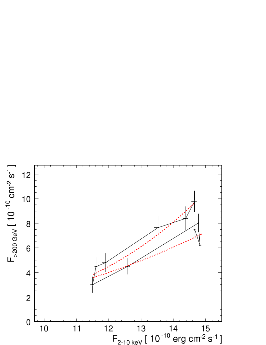
Figure 3: VHE flux versus the X–ray flux for the lightcurve shown in Figure 1. The correlation factor $r=0.86$ indicates that both wavebands are strongly correlated. There is an indication of a counter-clockwise pattern in this diagram where the VHE flux is lower in the rising part than in the decaying phase of the episode seen here. The decaying and the rising parts of the lightcurve are fitted to a power-law (dashed lines).

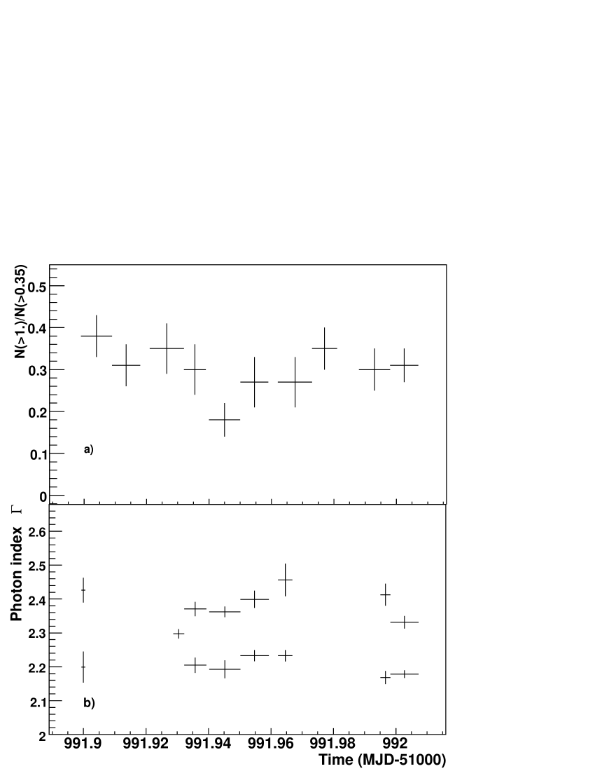
Figure 4: (a): Hardness ratio from the CAT data set, which is compatible with a constant. (b): Photon indices $\Gamma_{\rm L}$ and $\Gamma_{\rm H}$ on the same time scale as CAT where variability is evident for both indices due to their correlation with the flux. No correlation is exists between the VHE HR and the X–ray indices.

3.2 X–ray and optical variability

The optical data from the KVA telescope presented in (Sillanpää et al. 2001) had a few overlapping segments with the RXTE observations. The lightcurves of Fig. 5 show that there are no counterparts to the rapid and large variations seen in the X–rays, as has been mentioned in other similar multi-wavelenght studies. There is hence no evidence for simultaneous correlation between those wavebands, in agreement with other multi-wavelength campaigns carried out on this object (e.g. Błażejowski et al. 2005). The absence of correlation between simultaneous optical/VHE lightcurves is patent in other VHE emitting BL Lacs such as Mkn 501 (Petry et al. 2000), 1ES 1959+650 (Krawczynski et al. 2004) or PKS 2155-304 (Aharonian et al. 2005).

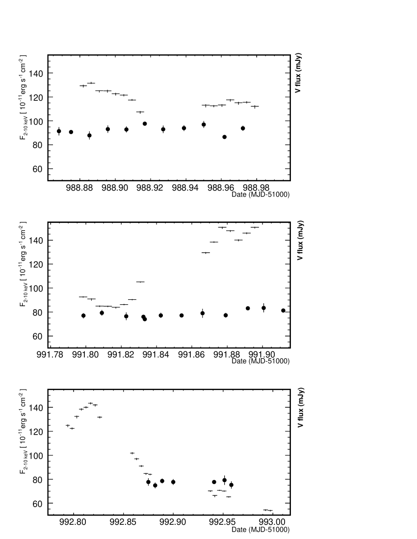
Figure 5: X–ray flux (crosses) and KVA optical flux (points), for 3 nights where observations overlapped. Note that the Y axis numbering is valid for both wavebands. The correlation factor $r=0.06$ indicates that both wavebands are not correlated, as is apparent in the lightcurves. When the 2-10 keV flux varies by more than 50% no such behaviour is visible in the optical.

To further investigate the energy-dependent variability, the fractional root mean square (rms) variability amplitude $F_{\rm var}$ (see e.g. Vaughan et al. 2003 for $F_{\rm var}$ and a derivation of the uncertainty $\sigma_{F_{\rm var}}$ in equation B2) is estimated for the X–ray and the optical lightcurves. $F_{\rm var}$ is defined by

$$F_{\rm var}=\sqrt{\frac{S^{2}-\overline{\sigma^{2}_{\mathrm{e}rr}}}{\bar{x}^{2}}}$$ (1)

where $s^{2}$ is the variance of the considered time series, $\sigma_{\mathrm{e}rr}$ is the mean square error of the flux measurements and $\bar{x}$ the mean of the flux.

Figure 6 shows $F_{\rm var}$ as a function of energy along with the optical KVA measurement of $F_{\rm var}=7.55\pm 0.71\%$, showing evidence for a power-law behaviour of $F_{\rm var}$ over four decades in energy with $F_{\rm var}\propto E^{0.24\pm 0.01}$. The increase in fractional variability with energy between 0.1-10 keV was previously noticed by Fossati et al. (2000a) using BeppoSAX data. Their X-ray fractional rms is also $\propto E^{1/4}$. The historical EUVE data point shown in Fig. 6, taken from the same intensive 1998 campaign on Mkn 421, is in very good agreement with the power-law trend.

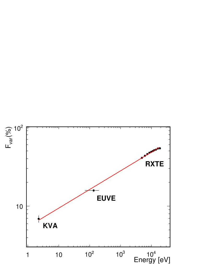
Figure 6: Fractional rms as a function of observed energy, for the RXTE and KVA data from this campaign. Also a EUVE measurement is shown as an open circle, from a MWL campaign on Mkn 421 (Takahashi et al. 2000) in 1998. The data are well described by a power law with a slope $\propto E^{1/4}$.

3.3 X–ray spectral patterns

It is commonly reported in blazar studies that the X–ray flux (or rate) correlates with the spectral index (or hardness ratio), indicating that the spectrum becomes harder when the flux increases. Since the X–ray data analysed here were fitted to a broken power law the flux dependency of 3 spectral parameters can be checked, namely the photon indices and the break energy $E_{\rm br}$. Surprisingly the break energy varies very little with time and also does not correlate with the flux, a fit to a constant yields a $\chi^{2}$ of 11.6 for 9 degrees of freedom, or a 23% chisquare probability. The distribution of $E_{\rm br}$ has an average value of $\overline{E_{\rm br}}=5.9\pm 1.1\,{\rm keV}$ independent of the flux.

The photon indices $\Gamma_{\rm L}$ and $\Gamma_{\rm H}$ however show some interesting features where the flux dependency is apparent up to a flux $F_{p}\approx 10^{-9}\,{\rm erg}\,{\rm cm}^{-2}\,{\rm s}^{-1}$ after which the indices appear to plateau (Fig. 7). Mentions of a possible hardness ratio saturation were made in George et al. (1988) and Nolan et al. (2004) but the datasets were insufficient to establish this behaviour.

A similar analysis was performed on Mkn 501 by Xue & Cui (2005) who derived the same broken power-law spectral parameters for that source and also found that the two photon indices show a spectral hardening and then level off at a flux of $F_{\rm p}\approx 5\times 10^{-10}\,{\rm erg}\,{\rm cm}^{-2}\,{\rm s}^{-1}$. The authors used a function consisting of a constant plus an exponential to describe the trend. This functional form does also fit quite well the Mkn 421 data shown here, as seen in the dashed lines in Figure 7.

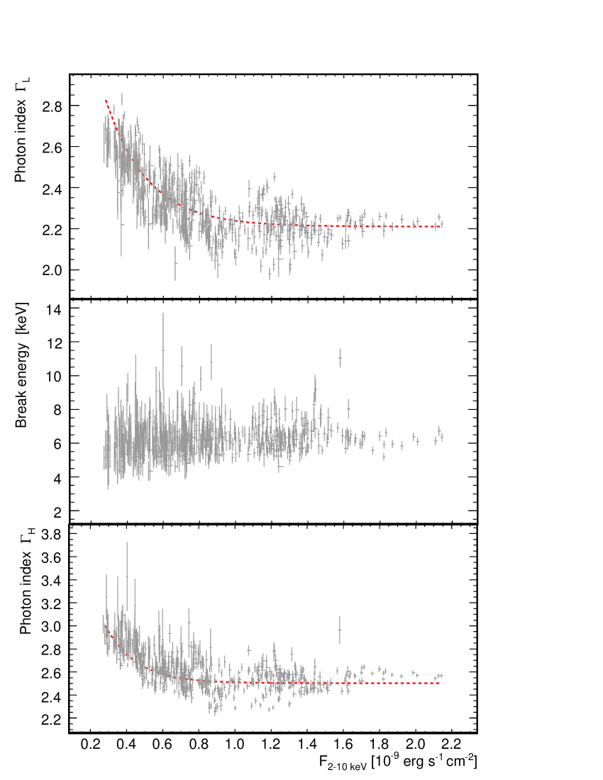
Figure 7: Dependence of the three spectral parameters on the flux, all derived from fits to a broken power law. The indices are seen to be levelling at some characteristic flux, whereas the break energy does not appear correlated with the flux.

The two photon indices are correlated ($r=0.99$) and a linear fit to the data set yields $\Gamma_{\rm H}\propto(0.96\pm 0.02)\times\Gamma_{\rm L}$ showing that the dependency is very linear, unlike the flux dependency found previously. The ratio between the two indices remains therefore constant throughout the whole observation sequence here, and is independent of the measured intensity. The part of the X-ray spectrum here appears to be pivoting around the 6 keV break energy, which is probably more an indication of a spectral curvature than a feature in the spectrum.

3.4 Resolved flares

As noted by Cui (2004) the shortest rise or decay times in Mkn 421 can be as short as 1000 s, but clearly resolved rising, peaking and decaying structures are not easy to define in the lightcurve due to the erratic exposure. There are however two rising and decaying structures visible in the intervals MJD 51987.0-51987.7 (flare A) and MJD 51992.6-51993.0 (flare B) with different amplitudes. Flare A’s flux is $\lesssim F_{p}$ whereas Flare B is $\gtrsim F_{p}$. This provides an interesting test for the spectral index behaviour: both flares start from a different baseline level, double their flux, and don’t exhibit the same spectral evolution: only the fainter flare shows a clear spectral evolution (Figure 8). The fact that the spectral index varies more when the flux is below the $F_{p}$ limit, both in the overall lightcurve as well as in resolved flares, will be discussed further in §4.4.

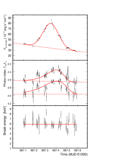
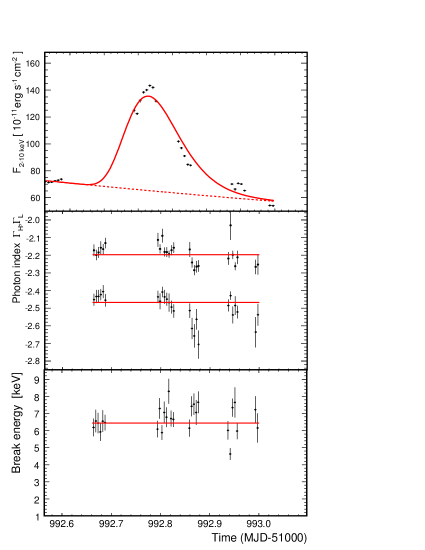
Figure 8: Spectral variations for a resolved flare where the flux is $\lesssim F_{p}$ (left panel) and $\gtrsim F_{p}$ (right panel). In the former case, both indices harden from their baseline value, peak later than the flux, and soften again with the characteristic hysteresis loop. The spectral indices are highest well after the flux peaks. In the latter case, no significant spectral variability is found when the flux doubles. The lines represent a fit of the flares to a lognormal function above a baseline modelled by an exponential decay (dashed line). These functions help to locate the extrema of the lightcurves but are not used to derive any physical parameters.

3.5 Time averaged spectrum

The CAT spectrum is derived from data between 300 GeV and 5 TeV, taken at zenith angles taken in the range $0^{\circ}-20^{\circ}$. The most probable spectrum for this data is $\frac{{\rm d}N}{{\rm d}E}=\Phi_{0}\times E^{-\alpha-\beta\times{\rm log}_{10}E/1{\rm TeV}}$ with $\Phi_{0}$=$(13\pm 0.85_{stat}\pm 2.76_{syst})\times 10^{-11}{\rm cm}^{-1}{\rm s}^{-1}{\rm TeV}^{-1}$, $\alpha$=$2.81\pm 0.09_{stat}\pm 0.07_{syst}$ and $\beta$=$0.79\pm 0.27_{stat}\pm 0.03_{syst}$. The curvature term is significant at $2.7\sigma$. The same data set can be fitted to a power law with an exponential cutoff yielding a similar likelihood with a cutoff energy of $E_{0}=1.4\pm 0.5\,{\rm TeV}$. The spectral curvature here is consistent with HEGRA (Aharonian et al. 2003) on Mkn 421 during these outbursts (though with a different time coverage) where a spectral cutoff at $E_{0}=3.4\pm 0.5\,{\rm TeV}$ at the $2.4\sigma$ level was reported. The Whipple data also show a curved spectrum (Krennrich et al. 2002) compatible with an exponential cutoff at $E_{0}=4.3\pm 0.3\,{\rm TeV}$ as well as the fact that there is no evidence for variation in the cutoff energy with flux. The difference in the value for $E_{0}$ from these experiments can be due to systematic effects (the errors quoted here are statistical only, all experiments give a systematic error on $E_{0}$ of $\sim 20\%$) and to the different observation times.

In order to derive a time-averaged X–ray spectrum consistent with the VHE spectrum, the RXTE data are reduced to obtain PCU-dependent PHA files constrained to start at the beginning of the first CAT run, and to end at the last run. The spectrum is fitted to a double broken power-law in XSPEC which yields a $\chi^{2}$ of 52.1 for 50 degrees of freedom, with an excellent chi-square probability of $P(\chi^{2})=0.39$. The spectral parameters are $\Gamma_{\rm L}=2.20\pm 0.06$, $\Gamma_{\rm M}=2.37\pm 0.10$, $\Gamma_{\rm H}=2.64\pm 0.04$, $E_{\rm br,1}=6.2\pm 0.1\,\rm keV$ and $E_{\rm br,2}=13\pm 1\,\rm keV$ where $\Gamma_{\rm M}$ is the photon index between the two break energies $E_{\rm br,1}$ and $E_{\rm br,2}$. Hence, there is significant curvature in the time-averaged X–ray spectrum, which is in agreement with earlier observations of Mkn 421 by telescopes such as ASCA (Tanihata et al. 2004) and BeppoSAX (Fossati et al. 2000b; Massaro et al. 2004). The 2-10 keV flux is $\approx 1.34\times 10^{-9}\,{\rm erg}\,{\rm cm}^{-2}\,{\rm s}^{-1}$.

The main facts that will be discussed now can be summarized as follows:

• The X-ray and VHE $\gamma$-ray fluxes are highly correlated within a time window of 3h.

• The optical flux rms, not its mean value, is correlated to the higher frequencies through its fractional RMS.

• The X-ray spectrum hardens with increasing flux only up to some characteristic level $F_{\rm p}$ after which it levels off.

4 Synchrotron self-Compton modelling of Mkn 421

VHE emission from BL Lac objects is typically interpreted as due to radiation from particles accelerated to high energies in a relativistic jet. The nature of the particles, their location(s), the acceleration mechanism(s), the radiative processes involved, etc, are all subject to debate. The simplest view is that of synchrotron self-Compton emission from electrons (positrons) located in a single, homogeneous zone. This view is adopted in the present work and confronted to the results accumulated in the previous section.

4.1 Constraints from the variability

Several simple constraints on the physical conditions in the emission zone may be obtained from the observations (e.g. Ghisellini et al. 1996). The observed variability timescale sets an upper limit to the emitting zone. The VHE doubling timescale of 30 minutes (Fig. 1) implies

$$R\delta^{-1}\leq 5.4\times 10^{13}\,{\rm cm}$$ (2)

where $R$ is the characteristic size of the region (assumed spherical in what follows) and $\delta$ is the boost factor from the bulk relativistic motion of the jet. The correlated X–ray and VHE emissions indicate that the emitting particles are likely to be co-spatial, and hence that the emitting volumes are similar. This is consistent with the hypothesis of a homogeneous emission zone.

The detection of $\gamma$-rays in the $0.3-10\,\rm TeV$ range implies that the opacity to pair production $\tau_{\gamma\gamma}$ within the emission region cannot significantly exceed 1, independently of the emission mechanisms. Following Tavecchio et al. (1998) the opacity $\tau_{\gamma\gamma}$ is

$$\tau_{\gamma\gamma}\approx\frac{\sigma_{\rm T}}{5}\frac{1}{hc}\frac{d_{L}^{2}}{R}\frac{1}{\delta^{3}(1+z)}F\left(E_{t}\frac{\delta^{2}}{(1+z)^{2}}\right).$$ (3)

In the above, $\tau_{\gamma\gamma}$ is the opacity seen by VHE photons with an observed energy $E_{\gamma}$. The VHE photons see a flux density $F(E_{t})$ of photons above the threshold for pair production $E_{t}=(m_{e}c^{2})^{2}/E_{\gamma}$, which occurs in the UV to X–ray range (observer frame). If the emission is co-spatial, the measured X–ray data can be used to estimate the flux density that VHE $\gamma$-rays may interact with. Imposing that $\tau_{\gamma\gamma}<1$ for photons with observed energy $E_{\gamma}=10\,\rm TeV$ and using Eq. 2 to constrain $R$ yields

$$\delta\geq 16.$$ (4)

The mean energy $E$ of synchrotron radiation from an electron with Lorentz factor $\gamma$ is given by $E\approx\frac{\delta}{1+z}\frac{21\hbar\gamma_{\rm e}^{2}qB}{15\sqrt{3}m_{e}}$ where $B$ is the magnetic field intensity in the emission zone. If the observed X-rays are synchrotron radiation from electrons then the maximum observed energy $E_{\rm max}=20\,\rm keV$, corresponding to the highest energy bin in the RXTE spectrum, yields

$$\gamma_{\rm max}\ga 1.4\times 10^{6}\,B^{-1/2}\delta^{-1/2}$$ (5)

In the SSC scenario, the same electrons should have enough energy to Comptonize ambient synchrotron photons up to the VHE regime, requiring

$$\frac{\delta}{1+z}\gamma_{\rm max}m_{e}c^{2}\approx 10\,{\rm TeV.}$$ (6)

Combining Eq. 5 and Eq. 6 yields a constrain on the magnetic field

$$B\delta^{-1}\leq 5.2\times 10^{-3}\,{\rm G}$$ (7)

which, for $\delta=16$, would imply $B\leq 0.08$ G and $\gamma_{\rm max}\ga 3.5\times 10^{5}$. This is of the order of the Lorentz factor derived in a similar way for Mkn 421 by Takahashi et al. (1996) who derived $\gamma_{\rm max}>5\times 10^{5}$ but lower than $\gamma_{\rm max}\approx 10^{7}$ found in a similar way in 1ES1959$+$650 (Giebels et al. 2002). Accommodating a higher magnetic field would require large relativistic speeds (boost factor $\delta$).

The relative strength of the inverse Compton (IC) contribution relative to the synchrotron ‘bump’ depends on the particle and magnetic field densities. Higher densities increase the IC emission while a higher $B$ increases the synchrotron contribution. In the Thomson regime, the relative luminosities are given by

$$\frac{L_{C}}{L_{S}}\approx\frac{(\nu F_{\nu})_{S}(d_{L}/R)^{2}/(c\delta^{4})}{B^{2}/8\pi}\ga 810\leavevmode\nobreak\ \delta_{16}^{-8}$$ (8)

where $B$ and $R$ are replaced by their maximum allowed value (Eqs. 2 and 7), $(\nu F_{\nu})_{S}\approx 2\times 10^{-9}$ erg s^-1 cm^-2 is the observed synchrotron spectral flux, $d_{L}\approx 4\leavevmode\nobreak\ 10^{26}$ cm is the luminosity distance, and the numerical application takes $\delta=16$ (Eq. 4). The small radius (high particle density) and low magnetic field implied by the constraints lead to a towering IC component, while both components are observed at roughly the same spectral luminosities. Therefore, this leads to values of $\delta$ closer to $\approx 40$ to match the relative luminosities.

In Mkn 421, inverse Compton emission at VHE energies occurs in the Klein-Nishina (KN) regime, where the electron gives away nearly all its energy to the photon. This regime is reached when the boosting electon has a Lorentz factor $\gamma$ such that $\gamma e^{\prime}_{S}\geq 1$ where $e^{\prime}_{S}$ is the energy of the target photon (in units of $m_{e}c^{2}$) in the jet flow frame. With synchrotron peaking at $\approx 500$ eV then $e^{\prime}_{S}\approx 10^{-3}\delta^{-1}$ and IC on electrons with $\gamma\geq 10^{3}\delta$ occurs in the KN regime. The IC cross-section then decreases dramatically so that the luminosity in Eq. 8 is overestimated. Nevertheless, the conclusion that a high value of $\delta$ is needed to fit the IC component should still hold: in the KN regime, the electrons will lead to a jet-frame peak IC luminosity $e^{\prime}_{IC}\approx 1/e^{\prime}_{S}$ (Georganopoulos & Kazanas 2003), which translates into $\delta\geq 30$ since $e^{\prime}_{IC}\approx 10^{6}\delta^{-1}$ (corresponding to about 0.5 TeV in the observer frame).

Hence, the VHE variability timescale and the SED imply large boosts $\delta\ga 30$, $R\sim 10^{15}$ cm and $B\sim 0.1$ G.

4.2 The standard SSC model

The validity of the above limit on $\delta$ is investigated using a numerical code calculating the homogeneous SSC emission from a given distribution of electrons in spherical geometry (Jones et al. 1974; Gould 1979; Band & Grindlay 1985). Radiative transfer is treated as in Kataoka et al. (1999). The Bessel functions, needed for the synchrotron emission and absorption coefficients (Rybicki & Lightman 1979), are computed using the Chebyshev expansion of MacLeod (1996). The Compton emissivity is computed using the Jones (1968) approximating kernel, which takes into account the reduction of the cross-section in KN regime and assumes an isotropic photon field. Absorption of VHE $\gamma$-rays due to pair production with the infrared extragalactic background light (EBL) during their propagation is taken into account. The pair production cross-section is given in Gould & Schréder (1967). The distribution and normalisation of the EBL are set to the upper limits found by the H.E.S.S. collaboration using observations of more distant TeV blazars (Aharonian et al. 2006).

The shape of the electron distribution is assumed to be a power-law with an exponential cutoff ${\rm d}N_{\gamma}\propto\gamma^{-s}\exp(-\gamma/\gamma_{b}){\rm d}\gamma$ from $\gamma_{\rm min}=1$ to $\infty$. The observed SED (Fig. 9) is power-law like from radio to optical with a spectral index $\alpha\approx 0.35$ ($S_{\nu}\propto\nu^{-\alpha}$). If the emission is synchrotron then the underlying electron power-law has an index $s\approx 1.7$. The decrease in spectral luminosity at X-rays implies a peak (in $\nu F_{\nu}$) synchrotron frequency somewhere in the extreme UV range (Tanihata et al. 2004). The corresponding $\gamma_{b}$ is univocally determined by adjusting to the data once $B$ and $\delta$ are set. It is typically of order $10^{5}$ as $\gamma_{b}\la\gamma_{\rm max}\approx 5\leavevmode\nobreak\ 10^{5}B^{-1/2}_{0.2}\delta_{40}^{-1/2}$ (Eq. 5 with $B=0.2$ G and $\delta=40$). Besides the shape of the particle distribution, the model parameters are the magnetic field $B$, the radius $R$, the boost $\delta$ and the particle density $n$. The first two are set to their maximal value allowed by constraints, depending on $\delta$ (Eqs. 2 and 7). This ensures IC emission is maximised. The only free parameters left are $\delta$ and $n$. Fits are attempted starting with $\delta=16$ and going upwards. Adequate fitting of the SED does require values above $\delta\approx 40$ as argued in §4.1.

The information gained by such modelling is limited. The particle distribution adjusted to fit the observations has $s\approx 1.7$ when values of 2–2.2 are the canonical values preferred theory-wise (Achterberg et al. 2001). Using $s\approx 2$ would require $\gamma_{\rm min}\sim 10^{3}$ (i.e. a limited range of non-thermal particles) in order not to overestimate the IR spectrum and enhance the HE $\gamma$-ray spectrum above the EGRET measurement. A high $\gamma_{\rm min}$ is not improbable as $\gamma_{\rm min}\sim\Gamma^{2}$ is expected for relativistic shock acceleration. Yet, one parameter is frozen (the index $s$) only to thaw another one ($\gamma_{\rm min}$) at the price of reproducing less of the SED: the exercise is not particularly enlightning.

The largest limitation is that such simple modelling is, by construction, unable to address the wealth of variability information gathered in the previous sections. Injection and cooling of particles has to be explicitely taken into account and compared to the spectral variability.

4.3 Evolved SSC model: steady-state

Particles are now continuously injected in a homogeneous sphere, losing energy to radiation until they escape after a time $t_{\rm esc}$ (Mastichiadis & Kirk 1997; Chiaberge & Ghisellini 1999). The evolution of the particle distribution $N(\gamma,t)$ is given by the diffusion equation

$$\frac{\partial N(\gamma,t)}{\partial t}=\frac{\partial}{\partial\gamma}\left[(\dot{\gamma}_{\rm s}+\dot{\gamma}_{\rm ic})N(\gamma,t)\right]+\frac{N(\gamma,t)}{t_{\rm esc}}+Q(\gamma)$$ (9)

where $\dot{\gamma}$ represents the radiative loss term to synchrotron and IC radiation, $N/t_{\rm esc}$ is the energy-independent escape term and $Q(\gamma)$ is the injected particle distribution. The radiative losses $\dot{\gamma}$ are computed from the synchrotron and IC power emitted by each electron, taking the Klein-Nishina drop in cross-section into account. The equation is solved using the Chang & Cooper (1970) algorithm (Park & Petrosian 1996). In all that follows the parameters are set to $\delta=40$, $B=0.2$ G and $R=2\times 10^{15}$ cm.

In the above, cooling will be unimportant if the particles escape before emitting a significant fraction of their energy. Taking into account only synchrotron radiation, the critical energy above which cooling is important is

$$\gamma_{\rm cool}=3\times 10^{5}\leavevmode\nobreak\ B_{0.2}^{-2}(ct_{\rm esc}/R)^{-1}.$$ (10)

Low-energy particles radiate away most of their energy if they are given the time. It can also be inferred from this equation that light travel time delays must be taken into account when investigating the emission of electrons with $\gamma\ga 3\times 10^{5}$, as these should cool on a time $\la R/c$ according to Eq. 10 above.

If the escape time is of order $R/c$ then the steady-state distribution is essentially the injected one because none of the particles cool significantly before escaping ($\gamma_{\rm cool}\sim\gamma_{\rm max}$). The situation is identical to §4.2. However, the gyroradius $R_{L}\approx 10^{10}\,\gamma_{6}B_{0.2}^{-1}$ cm of TeV electrons is very small compared to $R$ (Eq. 2), so it is more likely to have the electrons diffuse for some time in the emission region rather than see them escape on a direct flight. If $t_{\rm esc}\gg R/c$ the impact of cooling on the SED will be important.

Classically, with a power-law injection of particles $Q\propto\gamma^{-s}$ and $\dot{\gamma}\propto\gamma^{2}$ (synchrotron and Thomson IC), the steady-state ($t\rightarrow\infty$) distribution is a broken power-law with an index $s+1$ above $\gamma_{\rm cool}$. If, as diffusive shock acceleration suggests, $s=2$ up to some $\gamma_{\rm max}$, the cooled spectrum has $s=3$ and a flat SED from $h\nu_{\rm cool}\approx 13\leavevmode\nobreak\ \delta_{40}B_{0.2}^{-3}(ct_{\rm esc}/R)^{-2}$ keV up to $h\nu_{\rm max}$ ($>$20 keV, §4.1). A flat SED hardly fits the optical to X-ray range: Tanihata et al. (2004) find the emission is not flat but peaks in the UV. In addition, the emission below $\nu_{\rm cool}$ would still be a power-law with $\alpha=0.5$, inconsistent with observations.

The core problem in reproducing the SED with cooling power-laws is the large range of injected energies. There are too many low-energy electrons producing too much flux at optical frequencies and below. One remedy is to arbitrarily harden the injection to $s=1.7$ as done in §4.2, fine-tuning $\gamma_{b}$ so that the optical to X-ray transition is reproduced. As previously argued, this is not very satisfying. Another is to keep $s=2$ but increase $\gamma_{\rm min}$ so that high-energy particles carry more of the total injected energy, cutting off the low frequency emission. In the strong cooling regime where $\gamma_{\rm min}\geq\gamma_{\rm cool}$ there is no uncooled component in the distribution.

Injected particles over a limited energy range was found to work very well. In the limit of a mono-energetic injection, the steady-state particle distribution yields a power-law of index 1.7 for the chosen parameters, in excellent agreement with the observed SED. For synchrotron and Thomson cooling, the steady-state is well-known to be a power-law with an index 2. Here, inverse Compton cooling occurs in the less efficient KN regime, leading to a hardened equilibrium solution. That the mono-energetic injection naturally yields the right index without fine-tuning makes this solution extremely attractive.

In the following, relativistic Maxwellian injections (Saugé & Henri 2004; Katarzyński et al. 2006)

$$Q(\gamma)=K\gamma^{2}\exp(-2\gamma/\gamma_{b})$$ (11)

were adopted instead of strictly mono-energetic injections or power-laws over very limited ranges. The results are identical since the Maxwellian is strongly peaked at its characteristic energy $\gamma_{b}$. Maxwellians may arise from second order Fermi scattering on plasma waves or from acceleration during magnetic field reconnection (see §5).

Figure 9 shows the result of a fit to the simultaneous optical (KVA), X-ray (RXTE) and VHE (CAT) data, along with NED archival data and the time-averaged spectral measurement from the third EGRET catalog (Hartman et al. 1999). The contribution of the host galaxy at optical/IR was modelled following Katarzyński et al. (2003) as a blackbody of temperature $T$=3500 K, normalised to 7$\times 10^{-25}$ erg s^-1 cm^-2 at its peak. The injected Maxwellian distribution has $\gamma_{b}$=$1.6\times 10^{5}$ with $K=3.3\times 10^{-21}$ in Eq. 11. This is equivalent to an injection rate of $n_{\rm inj}=9.7\times 10^{-7}$ particles cm^-3 s^-1 or a total injected power $P_{\rm inj}=4\times 10^{39}$ erg s^-1.

In the strong cooling regime, the escape time sets the minimum energy up to which particles cool, given by $\gamma_{\rm cool}$ (taking both IC and synchrotron into account). With $t_{\rm esc}=50\leavevmode\nobreak\ R/c$ the synchrotron emission cuts off below optical and is unchanged above. The VHE emission is also unchanged but the GeV flux is lower as there are fewer low-energy seed photons. The adopted escape time is $t_{\rm esc}=5000\leavevmode\nobreak\ R/c$ so that particles cool down to $\gamma\sim 10$ before escaping, emitting low-frequency radio-waves.

This radio emission is self-absorbed in a one-zone model. If the radio emission zone is more extended (keeping the same $B$), the density of particles may be low enough to forego self-absorption. In general, the interpretation of the radio emission from blazars in SSC models requires the addition of an additional large-scale component representing the VLBI jet (Charlot et al. 2006).

The electron density in steady-state is $n_{\rm inj}t_{\rm esc}\approx 325$ particles cm^-3. The energy density in particles is about 5$\times 10^{-2}$  erg cm^-3 compared to a magnetic field energy density of 1.6$\times 10^{-3}$  erg cm^-3. A sub-equipartition magnetic field was also found by Maraschi et al. (1999) and appears generic of homogeneous models. The total luminosity is $\approx 1.5\times 10^{46}$  erg s^-1.

In conclusion, a steady-state homogeneous model with a Maxwellian-like injection of particles provides a simple description of the overall SED, removing the need to set-up a power-law with an arbitrary hard index. In the following, this picture is confronted with the constraints on variability derived in §3.

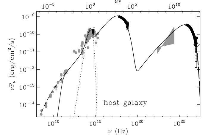
Figure 9: Simultaneous SED of Mkn 421 with archival EGRET (grey butterfly) and NED (grey points) data. The simultaneous VHE (CAT), X-ray (RXTE) and optical (KVA) data (§2) are highlighted in black. Most of the variability in the synchroton component occurs at X-ray energies (see Fig. 6) so that archival data below 1 eV, even if non-simultaneous, still provides valid constraints. The fit (solid line) is a steady-state homogeneous model assuming continuous injection of a Maxwellian distribution of electrons with $\gamma$=$5.3\times 10^{4}$ at a rate $n_{\rm inj}=9.7\times 10^{-7}$ particles cm^-3 s^-1 and cooling via synchrotron and self-Compton emission. The contribution of the host galaxy to the optical-IR (dotted line) is modelled using a blackbody spectrum as in Katarzyński et al. (2003). Values for the other parameters are $\delta=40$, $B=0.2\,{\rm G}$, $R=2\times 10^{15}\,{\rm cm}$ and $t_{\rm esc}=5000\,R/c$. The full line takes into account pair production on the EBL at VHE energies and synchrotron self-absorption at radio frequencies. The dashed line shows the unabsorbed model. Cooling in KN regime of the injected electrons leads to a steady-state distribution with the right slope to reproduce the radio to optical slope.

4.4 Evolved SSC model: variability

The observed variability decreases very rapidly with wavelength to only a few percent rms at optical (Fig. 6). X-rays should therefore provide the best constraints on the necessary modifications to explain the variability. The spectra corresponding to the highest and lowest X-ray fluxes measured in the campaign are shown in Fig. 10. This figure shows that the simultaneous detection of Mkn 421 by RXTE and CAT described earlier (Fig. 9) occurred while the X-ray flux was quite close to the maximum observed in this campaign.

A very good representation of the ‘low’ and ‘high’ SEDs is obtained by varying only the energy of the injected Maxwellian by about 50% from $\gamma_{b}=7.6\times 10^{4}$ (low) to $11.4\times 10^{4}$ (high), assuming that the source has time to reach steady-state (this is relaxed in §4.5). The coefficient $K$ (Eq. 11) is kept constant to its value of $3.3\times 10^{-21}$ found from fitting the simultaneous data. The injected power during the RXTE observations varies from 1.1$\times 10^{39}$–5.7$\times 10^{39}$ erg s^-1. Hence, the injection behaves ‘thermally’ with $n_{\rm inj}\propto\gamma_{b}^{3}$ or $P_{\rm inj}\propto\gamma_{b}^{4}$. The characteristic $\gamma_{b}$ is typically set by the balance of the radiative timescale with the acceleration timescale $t_{\rm acc}$ but it is unclear how this relates to $P_{\rm inj}$ without a detailed model for the acceleration process.

Varying $P_{\rm inj}$ or $n_{\rm inj}$, keeping $\gamma_{b}$ constant, alters the normalisation of the synchrotron and IC emission, but does not reproduce the spectral softening at X-rays with lower flux. Varying both $\gamma_{b}$ and $n_{\rm inj}$ (or $P_{\rm inj}$) is necessary to account for the SEDs. Adjusting both independently, there being no strong a priori reason why $n_{\rm inj}\propto\gamma_{b}^{3}$, still leads to this steep dependence.

No other single parameter change can reproduce the three SEDs. It is difficult to fathom why $t_{\rm esc}$, $R$, $B$ or $\delta$ would change on a timescale $R/c$ in the context of a one-zone model. In any case, varying these one at a time does not reproduce the evolution. Combined variations cannot be excluded, but the simplest solution is that the injected power fluctuates, giving rise to particles with characteristic energy $\gamma_{b}\propto P_{\rm inj}^{1/4}$.

The high and low model SEDs bracket the EGRET long-term average and have the same spectral slope. The VHE flux varies by an order-of-magnitude between low and high SEDs. The low VHE flux is consistent with the lowest measurements reported by Whipple and HEGRA (Macomb et al. 1995; Aharonian et al. 2002).

Figure 11 shows the fractional variation $f=(F_{\rm high}-F_{\rm low})/(F_{\rm high}+F_{\rm low})$ between the low and high SEDs. The strongest variability ($f\ga 0.5$) occurs between 1-100 keV and above about 100 MeV (EGRET band). The drop from 0.1 to 1 MeV is due to the increasing dominance of the IC component. Interestingly, $f$ increases as a power-law from IR to hard X-rays, just as observed in the rms variability vs energy plot (Fig. 6) but with a shallower slope. In particular, there is no feature associated with the synchrotron peak, which is around a keV and moves slightly to longer wavelengths with decreasing flux (Tanihata et al. 2004).

The variability in the IC component ($\ga$ 1 MeV) is less wavelength-dependent than the synchrotron component, as it mirrors primarily the changes in UV to X-ray seed photons. With $f\approx 0.3$ the optical variations are overestimated, although contamination from the host galaxy could reduce the measured variability from the expected value. Indeed, such a contribution is included in the plotted SEDs. It would produce a feature in the rms vs energy plot (Fig. 11), which seems unlikely since the extrapolation of the observed X-ray rms is spot on the optical. However, note that $f$ is not an rms. In principle, one should compute a theoretical lightcurve by varying $P_{\rm inj}$ according to some prescription and compare the rms vs energy theoretical plot (rather than $f$) with the observed one. Hence, detailed modelling of the rms plot can constrain how $P_{\rm inj}$ varies. The initial steps are described below but this is left for future work.

In conclusion, changes between high and low X-ray fluxes can be modelled as variations in the injected power of the pile-up distribution.

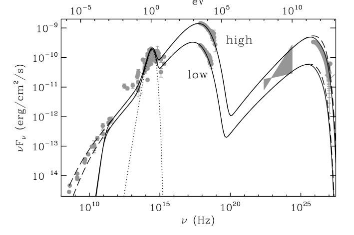
Figure 10: Non-simultaneous spectral energy distribution (SED) of Mkn 421 with the minimum and maximum X-ray fluxes detected in this campaign shown. Dashed lines are unabsorbed spectra. Dotted line is the host galaxy contribution. The ‘low’ and ‘high’ SEDs were fitted by varying the injected power $P_{\rm inj}$ in the steady-state homogeneous model, keeping all other parameters identical to those used for Fig. 9 (see §4.4). The injected particle energy behaves as $\gamma_{b}\propto P_{\rm inj}^{1/4}$. These changes result in wavelength-dependent variations between the two SEDs (see Fig. 11). At $\gamma$-ray energies, the SEDs bracket the long-term average measurement of EGRET. Variations in VHE flux by a factor $\sim 10$ between low and high states are expected.

Figure 11: Fractional flux variation between the low and high model SEDs in Fig. 10. The dashed line shows the expected dilution in IR-optical variability if the host galaxy contribution is taken into account. The dotted line represents the energy dependence of the rms variability found in Fig. 6. The fractional variation of the model (which is not an rms) has a shallower slope. The peak variations do not occur at the synchrotron peak but at the synchrotron frequency corresponding to the injection $\gamma_{b}$. IC becomes dominant above 1 MeV, producing a drop in variability. The IC variability is less wavelength-dependent since it mirrors changes in seed photons emitted from UV to X-ray wavelengths.

4.5 Towards the variability engine

Until now, particles have been considered to have time to reach steady-state, thereby neglecting any memory the system might have of its past condition. More realistically, variations in the injections will occur on timescales $\la R/c$ in order to reproduce the observed doubling timescale. Fluctuations in the engine power are mirrored in the emission of the VHE particles and then propagate down in wavelength as the particles cool. The system may not have time to adjust to the new conditions before another variation occurs. The SED received by the observer will depend on the history of fluctuations in injection.

It is beyond the scope of the present study to consider the resulting lightcurves for various prescriptions on how $P_{\rm inj}$ varies. Nevertheless, it is possible to illustrate the expected change in the limiting case of a response to a simultaneous, step-like change in injection throughout the emission region. Starting with the steady-state distribution corresponding to the high-state (resp. low-state) of Fig. 10, the injection $\gamma_{b}$ is abruptly set to its low-state (resp. high-state) value after some arbitrary time. The resulting lightcurves at various energies are shown in Fig. 12. While the change in injection is simultaneous throughout the emission zone, an observer would see the impact of the variation first on the closest part of the sphere and see a change on the opposite side after a time $R/\delta c$ (e.g. Chiaberge & Ghisellini 1999). This light propagation effect is taken into account when computing the lightcurves, following Kataoka et al. (2000).

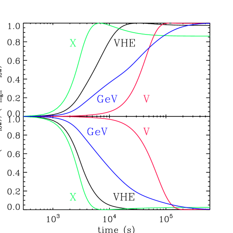
Figure 12: Lightcurve response to a step change in the injection of particles from low-to-high state (top) and from high-to-low state (bottom). The injected $\gamma_{b}$ is abruptly changed at $t=0$ simultaneously throughout the emission region. Light propagation delays are taken into account and time is counted in the observer frame. The X-ray lightcurve is integrated from 2-10 keV, VHE is the integrated flux above 200 GeV, GeV is the integrated flux between 100 MeV and 10 GeV, V is the optical $V$ band flux. Note the rapid response of the X-ray and VHE flux, the $\sim$1 day delay at optical and the gradual response of the flux in the EGRET band. Correlations between X-ray/VHE can be expected. However, the long delays and slower rates of change will hide correlations with the optical or GeV fluxes.

As expected, the response is quickest at X-rays and VHE, corresponding to electrons with the highest energies. This explains the correlations between these bands. The impact of the change in injection only propagates down to the optical $V$ band after a delay of $\sim$ a day, as previously discussed in Mastichiadis & Kirk (1997). This large delay would explain the lack of correlations between X-rays and optical bands. The rate of change is a few ks for the X-rays whereas it takes a few tens of ks for the optical to drop. Sputters in the variability engine on a timescale $\la 10$ ks will be smoothed out in the optical compared to X-rays, further reducing the amplitude of the variations at optical compared to the estimate made in Fig. 11. At GeV energies, the variation is also delayed and very gradual as the IC emission results from an integration over the seed spectrum. Variations at GeV could be even smoother in time than at optical wavelengths. Quantitative estimates of these aspects require a full simulated lightcurve.

The correlation between the X-ray and VHE lightcurves is shown in Fig. 13 for step changes. The finite light travel time and slightly different cooling combine to produce an asymmetric loop. At the other extreme, a change in particle injection could occur at a slow enough pace that the particles are in steady-state, at least at those energies. Looking at Fig. 12, this will typically require variations in the injection on timescales of many ks. In this case, $P_{\rm inj}$ is slowly varied between its two extreme values. The flux evolution is plotted in Fig. 13. Differences between low-to-high and high-to-low disappear as the SED is in steady-state at all times. The correlation is well approximated by $F_{\rm VHE}\propto F_{\rm X}^{1.3}$, as expected for SSC in the Klein-Nishina regime where $L_{\rm IC}$ is proportional to the number of electrons rather than its square (Ghisellini et al. 1996). This is very close to the long-term trends discussed in §3.1. Steeper dependences of the VHE flux with X-ray flux on short timescales, as found in the CAT data, are not explained to satisfaction here. The limited dynamic range may bias the dependences found in datasets with a short time base (Katarzyński et al. 2005). Inversely, these may be able to shed more light on the workings of the engine than long-term averages. As with the energy dependence of the rms, computing lightcurves given some prescription for variations in $P_{\rm inj}$ would be needed to properly investigate the issue.

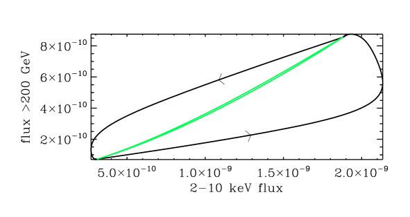
Figure 13: Correlation between X-ray and VHE fluxes plotted in Fig. 12. The black curve shows the correlation for step changes from a low steady-state (bottom left) to a high steady-state (top right) and back. Arrows indicate the low-to-high and high-to-low direction in which the loop is traced. The correlation is not symmetric because of light propagation delays. The grey curve illustrates the other extreme case in which variations occur on a timescale $>10$ ks so that the highest energy particles always reach steady-state. In this case, the light travel time and cooling effects have no influence and the change is symmetric. The correlation is then found to follow $F_{\rm VHE}\propto F_{\rm X}^{1.3}$, as expected of IC in the Klein-Nishina regime.

Figure 14 shows the evolution of the X-ray spectral indices $\Gamma_{\rm L}$ (2-6.5 keV) and $\Gamma_{\rm H}$ (6.5-10 keV) in the model for the step-like and slowly varying cases. There is a flattening above $\sim 10^{-9}$ erg s^-1 cm^-2 when the variation goes from low-to-high. There is no such flattening in the opposite direction. The reasons are not obvious and are related to the interplay between injection, cooling and light propagation. Nevertheless, variations in index should occur within this loop, in agreement with the observations (Fig. 7).

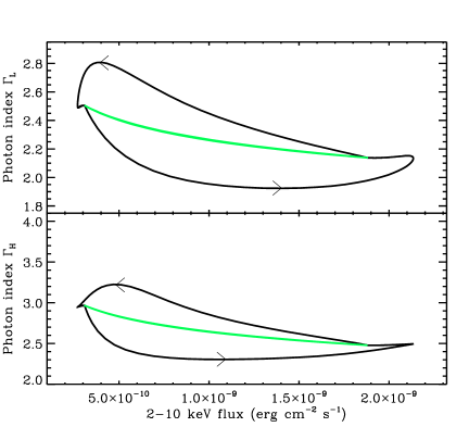
Figure 14: Correlation between X-ray photon indices $\Gamma_{\rm L}$ (top panel) and $\Gamma_{\rm H}$ (bottom panel) with the 2-10 keV flux. The black solid line corresponds to step changes in the injection, while the grey solid line is for an injection varying on a timescale $\gg R/c$ (as in Fig. 13). The direction of change from low-to-high and back are illustrated by arrows. The observed indices and fluxes shown in Fig. 7 (on the same scale) fall within the dark loop.

In conclusion, the fits made in §4.4 are used to study the response to variations in the injection from the low to the high-state values and back. The variations are assumed to be either instantaneous (step-like) or slow enough for the high-energy electrons to reach steady-state, thereby illustrating two extreme cases. Fluctuations in X-ray and VHE $\gamma$-ray fluxes are found to be correlated with an index identical to the one derived from long time-base observations. The expected variations in X-ray photon index vs flux also agree well with the observations. The GeV and optical suffer long delays and respond much more slowly to sudden changes, which should decrease their variability amplitude and hide correlations with X-rays or VHE $\gamma$-rays. Hence, the essence of the observational results garnered in §3 can be reproduced with a simple change in injected non-thermal power $P_{\rm inj}$, assuming the distribution is Maxwellian with a peak energy $\gamma_{b}\propto P_{\rm inj}^{1/4}$.

5 Discussion

The CAT observations presented here confirm that fast variability on timescales $\la 1$ hr is a hallmark of VHE emission from Mkn 421. Nevertheless, the dataset remains limited compared to X-rays, making the identification of a characteristic timescale uncertain. Rapid X-ray flaring, down to sub-hour timescales, appears to be assocated with high X-ray fluxes – which is also when Mkn 421 is detected by Cherenkov telescopes (Cui 2004). At lower fluxes, X-ray variability seems to occur on longer timescales (Takahashi et al. 2000). Observations with long time-bases and at lower fluxes are needed to characterize better the variability properties at VHE energies and compare them to the X-ray properties.

As with other BL Lac objects, the limit from internal absorption of $\gamma$-rays implies a high relativistic bulk motion in the jet $\delta>16$. Even higher values of $\delta\approx 40$ are required to model the simultaneous CAT, RXTE and optical SED with a single-zone, homogeneous SSC model. These higher values are needed to ensure that the emission zone is large enough, hence densities low enough, to avoid over-producing $\gamma$-ray emission by inverse-Compton emission. The emission region size $R=2\times 10^{15}$ cm is smaller and the magnetic field intensity $B=0.2$ G slightly higher than that found in previous works (Takahashi et al. 1996; Mastichiadis & Kirk 1997; Maraschi et al. 1999; Chiaberge & Ghisellini 1999; Katarzyński et al. 2003; Konopelko et al. 2003).

High values for $\delta$ contrast with the kinematics deduced from radio VLBI observations, which typically imply Doppler factors of a few at larger scales. VLBA measurements of Mkn 421 realised shortly after the high VHE state reported here did not find any new components at the parsec scale after the VHE high state in 2001 (Piner & Edwards 2005). Solutions to this inconsistency include strong jet deceleration between the $\gamma$-ray emitting zone and the parsec scale (Georganopoulos & Kazanas 2003), or a fast-moving spine surrounded by a slower-moving sheath (Chiaberge et al. 2000). However, high $\delta$ factors are likely inherent to single-zone SSC models and more complex, inhomogeneous model can be expected to reduce the discrepancy (Henri & Saugé 2006).

The spectral variability of Mkn 421 is investigated under the assumption of continuous injection of high energy electrons in the emission region. Mastichiadis & Kirk (1997) and Chiaberge & Ghisellini (1999) had used injection functions $Q\propto\gamma^{-s}\exp(-\gamma/\gamma_{b})$ with $s\approx 1.7$ set in order to reproduce both the synchrotron X-rays and the power-law at lower energies. This is a harder value than expected for the power-law distributions resulting from diffusive shock acceleration.

A Maxwellian injection naturally yields a cooling distribution with an index $s\approx 1.7$, forfeiting the need to arbitrarily set an injection index. Pile-ups arise naturally from stochastic acceleration (second-order Fermi acceleration) on plasma wave turbulence and can be as effective in producing high energy particles as first-order Fermi acceleration at shocks (Schlickeiser 1984, 1985; Aharonian et al. 1986). Quasi-monoenergetic injections may also be expected from reconnection in Poynting-flux dominated jets (e.g. Sikora et al. 2005 and references therein).

The substantial X-ray spectral variations are well reproduced by a factor $\approx$ 5 change in injected power. The characteristic energy of the particles $\gamma_{b}$ varies as $P_{\rm inj}^{1/4}$. A thermal-like correspondence between total injected power and characteristic energy of the VHE particles is surprising: even if the acceleration process results in a pile-up distribution, why should the injection rate vary as $\gamma_{b}^{3}$ ? Whether this is a coincidence or something which to be addressed by acceleration theory remains to be decided.

The injected particles have a characteristic $\gamma_{b}\sim 10^{5}$, which corresponds to the minimum energy for which electrons cool in a time $\la R/c$, and which also correponds to the maximum energy that can be reached in the acceleration process before cooling dominates. This suggests that $t_{\rm acc}\sim t_{\rm cool}\sim R/c$. Symmetric rise and decay lightcurves are expected in this case at X-ray energies (Chiaberge & Ghisellini 1999), as observed in Mkn 421 (Cui 2004).

The higher $\gamma_{b}$ hints at a decreasing $t_{\rm acc}$, hence a more efficient particle acceleration mechanism in the high state. This also explains the saturation of the X-ray spectral indices above a certain flux. The index varies less when the synchrotron peak reaches the spectral band. Such a saturation has also been observed in Mkn 501. A detailed comparison between these and other sources could provide simpler diagnostics of acceleration at the highest energies than hysteresis loops (e.g. Fig. 13). Both clockwise and counter-clockwise loops have been seen in Mkn 421 (Takahashi et al. 1996; Fossati et al. 2000b; Cui 2004). The choice of spectral bands and the base-line emission may significantly affect the resulting loops and make them ambiguous to interpret as isolated cooling/heating events, whereas an overall flux - index plot for the whole dataset may provide a broader, simpler picture to address.

Likewise, the power-law dependence of the fractional variability with energy from optical to X-ray energies may offer new insights into the workings of the engine. It does not imply correlations between the lightcurves at all these energies (i.e. the phase information can be lost). Indeed, the relationship between rms variability and energy seems unlinked to the flux level. In the present model, the engine must somehow be able to wag the high energy tail of the particle distribution in the right way so that the variation propagates down in energy with a tightly-constrained decreasing amplitude. Theoretical lightcurves, obtained by varying $P_{\rm inj}$, should be computed and their rms compared to the observations. Interestingly, the slow response of the GeV flux to step changes in injection suggests strong variations at X-ray and TeV energies which may not be accompanied by similar variations at GeV energies. Characterizing the amplitude and correlation with other bands by detailed modelling will be useful for GLAST.

6 Conclusion

Simultaneous observations carried out with CAT and RXTE confirm the correlation between X-ray and VHE emission and the fast sub-hour variability at VHE energies. A saturation of the X-ray spectral indices with X-ray flux and a power-law relationship between fractional variability and energy (from optical to X-rays) are found. These results may extend to other TeV blazars, and thereby provide strong, universal constraints on models of high energy emission from relativistic jets.

The SED and variability are well reproduced by a single-zone, homogeneous model in which a Maxwellian distribution of electrons with $\gamma_{b}\sim 10^{5}$ are continuously injected. Such an injection would favour second-order Fermi acceleration or neutral point acceleration over the more widely studied shock acceleration. Cooling by synchrotron self-Compton emission in the Klein-Nishina regime naturally leads to a steady-state distribution of electrons with the correct slope to explain the emission down to radio frequencies. The X-ray spectral saturation and power-law rms spectrum are reproduced by a factor 5 change in the power $P_{\rm inj}\propto\gamma_{b}^{1/4}$ of the injected Maxwellian. The acceleration process is probably responsible for this dependence, while variations in $P_{\rm inj}$ depend on the workings of the internal engine. Detailed lightcurves, particularly at $\gamma$-ray energies where the information is sparse, can therefore provide important insights into the mechanisms at work in blazars.