Polarimetric standardization

Abstract

The use of polarimetric techniques is nowadays widespread among solar and stellar astronomers. However, notwithstanding the recommandations that have often been made about the publication of polarimetric results in the astronomical literature, we are still far from having a standard protocol on which to conform. In this paper we review the basic definitions and the physical significance of the Stokes parameters, and we propose a standardization of the measurement of polarized radiation.

¹ Dipartimento di Astronomia e Scienza dello Spazio, Università degli Studi di Firenze, Largo Enrico Fermi 2, I-50125 Firenze, Italy
² European Southern Observatory, Alonso de Cordova 3107, Vitacura, Santiago, Chile
³ Institut fuer Astronomie, Universitaet Wien, Tuerkenschanzstrasse 17, A-1180 Wien, Austria

1. Introduction

The polarization properties of a radiation beam can be described in several different ways but have ultimately to rely on the specification of four independent quantities. Particularly suitable from this point of view are the so-called Stokes parameters which were introduced in the scientific literature by George Gabriel Stokes Stokes52 (1852) and which are commonly referred to, in modern notations, with the symbols $I$, $Q$, $U$, and $V$. It is possible to give two different definitions for the Stokes parameters of a beam of electromagnetic radiation propagating along a given direction. According to the first one, the Stokes parameters are expressed as statistical averages of bilinear products of the components of the electric field along two perpendicular axes, both perpendicular to the direction of propagation of the radiation (see Sect. 3). This basic definition is also used in practice by radio-astronomers for expressing their measurements of the Stokes parameters. The second definition, mostly used by optical astronomers, is an operational one that makes use of the concept of ideal filters (see Sect. 7). Obviousy, the two definitions have to be consistent.

2. The choice of the reference system

Before introducing these two definitions, it is fundamental to point out that both of them need the preliminary choice of a reference direction pertaining to the plane perpendicular to the direction of propagation of the radiation. To introduce the first definition of the Stokes parameters (the one based on bilinear products of the components of the electric field), we refer to a right-handed coordinate system, ($x,y,z$), with the $z$-axis directed along the direction of propagation and the $x$-axis directed along the reference direction. In astronomical observations, the reference direction can be thought of as the great circle pertaining to the celestial sphere and passing through the observed object. Though the choice of the great circle is, in principle, arbitrary, it has become customary, at least in night-time astronomy, to choose the reference direction as the celestial meridian passing through the observed object. In solar observations this convention is not always followed since there are, in general, more physical directions to choose, like the tangent to the solar limb for prominence observations, or the direction passing through the observed point and the center of the solar disk for sunspots observations. In polarimetric measurements of other solar system objects (e.g., asteroids) it is common to adopt as reference direction the great circle passing through the object itself and the Sun, or, better choice, the perpendicular to it (see Sect. 6).

3. The basic definition

According to Maxwell equations, the electric field vector of the radiation beam lies in the $(x,y)$ plane so that it is described by only the two components $E_{x}$ and $E_{y}$. In a fixed point of space along the direction of propagation, at the entrance of the telescope for instance, these two components of the electric field are described by the functions of time, $E_{x}(t)$ and $E_{y}(t)$, for which we can introduce the Fourier transforms, ${\cal E}_{x}(\omega)$ and ${\cal E}_{y}(\omega)$, according to the usual definitions

$$\begin{array}[]{rcl}{\cal E}_{x}(\omega)&=&\int_{-\infty}^{\infty}E_{x}(t)\,{\rm e}^{-{\rm i}\omega t}\,{\rm d}t\\ {\cal E}_{y}(\omega)&=&\int_{-\infty}^{\infty}E_{y}(t)\,{\rm e}^{-{\rm i}\omega t}\,{\rm d}t\;\;.\\ \end{array}$$ (1)

The Stokes parameters of the radiation beam at the angular frequency $\omega$ are defined by the expressions

$$\begin{array}[]{rcl}I(\omega)&=&\phantom{{\rm i}}k\,[\langle{\cal E}_{x}(\omega)^{*}{\cal E}_{x}(\omega)\rangle+\langle{\cal E}_{y}(\omega)^{*}{\cal E}_{y}(\omega)\rangle]\\[5.69054pt] Q(\omega)&=&\phantom{{\rm i}}k\,[\langle{\cal E}_{x}(\omega)^{*}{\cal E}_{x}(\omega)\rangle-\langle{\cal E}_{y}(\omega)^{*}{\cal E}_{y}(\omega)\rangle]\\[5.69054pt] U(\omega)&=&\phantom{{\rm i}}k\,[\langle{\cal E}_{x}(\omega)^{*}{\cal E}_{y}(\omega)\rangle+\langle{\cal E}_{y}(\omega)^{*}{\cal E}_{x}(\omega)\rangle]\\[5.69054pt] V(\omega)&=&{\rm i}k\,[\langle{\cal E}_{x}(\omega)^{*}{\cal E}_{y}(\omega)\rangle-\langle{\cal E}_{y}(\omega)^{*}{\cal E}_{x}(\omega)\rangle]\\ \end{array}$$ (2)

where $k$ is a positive constant, the symbol $*$ means complex conjugate, and the symbol $\langle\cdots\rangle$ means a statistical average which is implicit in the process of measurement.

There are some risks of ambiguity in the definition of Stokes parameters. One of course is the choice of the handedness of the reference system. We have adopted a right handed reference system, but adopting a left handed system will change the signs of $U$ and $V$.

There is a much more subtle ambiguity arising from the definition of Fourier transform. In our definitions of Eq. (2) we have implicitely adopted for the Fourier transform the representation of Eq. (1). Introducing the alternative definition with the substitution

$${\rm e}^{-{\rm i}\omega t}\rightarrow{\rm e}^{{\rm i}\omega t}\;\;$$

namely, defining

$$\begin{array}[]{rcl}{\cal E}^{\prime}_{x}(\omega)&=&\int_{-\infty}^{\infty}E_{x}(t)\,{\rm e}^{{\rm i}\omega t}\,{\rm d}t\\[5.69054pt] {\cal E}^{\prime}_{y}(\omega)&=&\int_{-\infty}^{\infty}E_{y}(t)\,{\rm e}^{{\rm i}\omega t}\,{\rm d}t\\ \end{array}$$ (3)

one obviously has, being $E_{x}(t)$ and $E_{y}(t)$ real,

$$\begin{array}[]{rcl}{\cal E}^{\prime}_{x}(\omega)&=&{\cal E}_{x}(\omega)^{*}\\ {\cal E}^{\prime}_{y}(\omega)&=&{\cal E}_{y}(\omega)^{*}\\ \end{array}$$

so that the sign of the $V$ Stokes parameter changes when the definition of the Fourier transform is changed from Eq. (1) to Eq. (3). In practice, this means that when adopting Eq. (2) for the definition of the Stokes parameters, one has to be aware that such definition implies a convention about the choice of positive or negative time in the definition of the Fourier transform.

Finally, we want to comment on the use of an arbitrary constant in front of the bilinear expressions that defines the Stokes parameters. As a matter of fact, we always use relative quantities, that is, we normalise $Q$, $U$, and $V$ to the intensity, and we consider the reduced Stokes parameters $P_{Q}$, $P_{U}$, and $P_{V}$ defined by

$$\begin{array}[]{rcl}P_{Q}&=&Q/I\\ P_{U}&=&U/I\\ P_{V}&=&V/I\\ \end{array}$$ (4)

so the value of the constant $k$ can be left undefined.

4. The physical significance of the Stokes parameters

According to the definition given by Eqs. (2), Stokes $Q$ is the difference between the amount of photons whose electric field oscillates along the reference direction and the amount of photons whose electric field oscillates in the direction perpendicular to it; Stokes $U$ is the difference between the amount of photons whose electric field oscillates at $45^{\circ}$ and the amount of photons whose electric field oscillates at $135^{\circ}$ with respect to the reference direction (the angles are reckoned counterclockwise from the reference direction looking at the source – see Fig. 1).

Stokes $V$ is given by the so called right handed circular polarization minus the left handed circular polarization, that are so defined: in a fixed point of space, the tip of the electric field vector carried by a beam having positive circular polarization rotates clockwise, as seen by an observer looking at the source of radiation. Viceversa, the tip of the electric field vector carried by a beam having negative circular polarization rotates counterclockwise, as seen by an observer looking at the source (see Fig. 1).

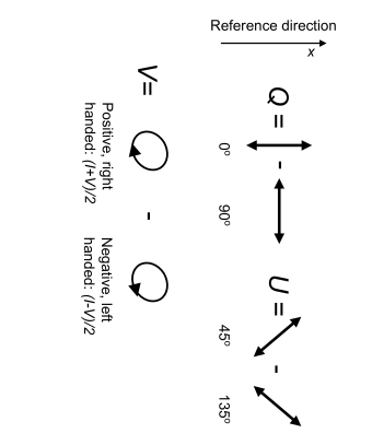
Figure 1.: Geometrical visualization of the definition of Stokes parameters. The observer is looking toward the source.

It is possible to show that Stokes parameters give information about the ellipse drawn by the tip of the electric vector in the plane perpendicular to the direction of wave propagation. For the sake of simplicity, one can consider the case of a monochromatic wave, which is completely polarized. More generally, we remind that any radiation beam can be considered as the incoherent superposition of an unpolarized beam and a beam which is totally polarized (Chandrasekhar theorem). The tip of the electric field associated with this beam draws, in a fixed point of space, an ellipse. The major and minor semi-axes of this ellipse, $a$ and $b$, (expressed in non dimensional units), and the tilt angle, $\theta$, that the major semi-axis forms with the reference direction $x$ (reckoned counterclockwise -for an observer looking at the source- from the reference direction) are connected to the reduced Stokes parameters of the polarized component by the equations

$$\begin{array}[]{rcl}a&=&\frac{1}{2}\left[(1-P_{V})^{1/2}+(1+P_{V})^{1/2}\right]\\[5.69054pt] b&=&\frac{1}{2}|(1-P_{V})^{1/2}-(1+P_{V})^{1/2}|\\[5.69054pt] P_{U}/P_{Q}&=&\tan\left(2\theta\right)\\ \end{array}$$ (5)

where $|z|$ means absolute value of $z$. Stokes $V$ is connected to the eccentricity of the polarization ellipse, and Stokes $Q$ and $U$ tell us how the polarization ellipse is oriented. If linear polarization is zero, the polarization ellipse degenerates in a circle. If circular polarization is zero, the polarization ellipse degenerates in a segment.

5. Linear polarization and position angle

Linear polarization is often expressed also in terms of $P_{\rm L}$ and $\theta$, where $P_{\rm L}$ is the fraction of linearly polarized radiation, and $\theta$ is the angle of maximum polarization, i.e., the angle that the major axis of the polarization ellipse forms with the $x$-axis of the reference system reckoned with the usual convention:

$$\begin{array}[]{rcl}P_{\rm L}&=&\sqrt{P_{Q}^{2}+P_{U}^{2}}\\ P_{Q}&=&P_{\rm L}\,\cos(2\theta)\\ P_{U}&=&P_{\rm L}\,\sin(2\theta)\\ \end{array}$$ (6)

The use of $P_{\rm L}$ and $\theta$ is widespread in astronomy because it allows the graphical superposition of linear polarization results to the image of the observed object. Note that from Eq. (6) one may be tempted to calculate the position angle $\theta$ as $(1/2)\,\arctan(P_{U}/P_{Q})$. This is incorrect, as can be seen with the following example: consider the case of $\theta=67.5^{\circ}$ i.e., a polarization ellipse with its major axis tilted at an angle of $67.5^{\circ}$ with respect to the reference $x$-axis. From Eq. (6), we obtain $P_{Q}=-P_{\rm L}/\sqrt{2}$ and $P_{U}=P_{\rm L}/\sqrt{2}$. By blindly computating $(1/2)\,\arctan(P_{U}/P_{Q})$ one will find an ellipse tilted at $-22.5^{\circ}$, i.e., perpendicular to the original, correct one. The reason for that inconsistency is that arctan is a function defined between $-90^{\circ}$ and $90^{\circ}$. The correct expression for obtaining the position angle (apart from inessential multiples of $\pi$) is the following one:

$$\begin{array}[]{rcll}\theta&=&+\frac{1}{4}\pi&\mathrm{if}\ P_{Q}=0\ \mathrm{and}\ \ P_{U}>0\\ \theta&=&-\frac{1}{4}\pi&\mathrm{if}\ P_{Q}=0\ \mathrm{and}\ \ P_{U}<0\\ \theta&=&\frac{1}{2}\arctan\left(\frac{P_{U}}{P_{Q}}\right)&\mathrm{if}\ P_{Q}>0\\ \theta&=&\frac{1}{2}\arctan\left(\frac{P_{U}}{P_{Q}}\right)+\frac{\pi}{2}&\mathrm{if}\ P_{Q}<0\\ \end{array}$$ (7)

Alternatively, one can substitute Eqs. (7) by the unique formula, suggested by V. Bommier (private communication)

$$\theta={1\over 2}\,{\rm sign}(P_{U})\,\arccos\left(\frac{P_{Q}}{\sqrt{P_{Q}^{2}+P_{U}^{2}}}\right)\;\;.$$ (8)

6. Transforming Stokes parameters into a new reference system

A further point concerns the transformation law for the Stokes parameters when changing the reference direction. If the new reference direction is obtained from the old one by a counterclockwise (looking at the source) rotation of an angle $\chi$, by means of Eq. (2) one can easily show that the new reduced Stokes parameters, $(P_{Q}^{\prime},P_{U}^{\prime},P_{V}^{\prime})$, are connected to the old ones, $(P_{Q},P_{U},P_{V})$, by the equations

$$\begin{array}[]{rcl}P_{Q}^{\prime}&=&\cos\,(2\chi)\,P_{Q}+\sin\,(2\chi)\,P_{U}\\ P_{U}^{\prime}&=&-\sin\,(2\chi)\,P_{Q}+\cos\,(2\chi)\,P_{U}\\ P_{V}^{\prime}&=&P_{V}\\ \end{array}$$ (9)

Equations (9) show that the linear polarization Stokes parameters, $Q$ and $U$, transform between each other when the reference direction is changed, whence the importance, as already remarked, of clearly specifying the chosen reference direction when publishing a result concerning linear polarization. The same equations also show the invariance of the quantity $P_{\rm L}$ under a rotation of the reference direction, and the obvious fact that a rotation of the reference direction of $180^{\circ}$ leaves all the Stokes parameters invariant. This last fact means that when choosing the reference direction it is not necessary to specify “an arrow” on the direction itself. If, for instance, one chooses as reference direction the celestial meridian passing through the observed object, it does not matter whether the $x$-axis of the system $(x,y,z)$, on which the electric field components are defined, is directed towards the North or the South pole.

It should be noted that Eq. (9) says that the position angle $\theta$ represents the angle by which one should rotate the reference direction (in the counterclockwise direction, looking at the source), in order to end up with a positive $P_{Q}$ value (which indeed turns up to be equal to $P_{\rm L}$) and a null $P_{U}$ value.

As an example of the use of Eq. (9), let us consider the polarization of a solar system object measured in a system that has the reference direction ($x$-axis) aligned to the celestial meridian passing through the observed object. We want to transform Stokes parameters into a system that has the reference direction perpendicular to the great circle passing through the object and the Sun. We have to calculate $P_{Q}^{\prime}$, $P_{U}^{\prime}$, $P_{V}^{\prime}$ via Eqs. (9), setting $\chi=\Phi+\pi/2$, where $\Phi$ is the angle between between the celestial meridian passing through the object and the great circle passing through the Sun and the object. The angle $\Phi$ is related to the coordinates of the object and of the Sun through the relationship

$$\sin\delta_{\rm T}\cos(\alpha_{\odot}-\alpha_{\rm T})=\tan\delta_{\odot}\cos\delta_{\rm T}-\sin(\alpha_{\odot}-\alpha_{\rm T})\frac{1}{\tan\Phi}$$ (10)

where $(\alpha_{\odot},\delta_{\odot})$, and $(\alpha_{\rm T},\delta_{\rm T})$ are the right ascension and declination of the Sun, and of the observed object, respectively. Alternatively, one can directly calculate

$$\begin{array}[]{rcl}P_{Q}^{\prime}&=&\frac{{\cal B}^{2}-{\cal C}^{2}}{1-{\cal A}^{2}}\,P_{Q}-\frac{2\,{\cal B}{\cal C}}{1-{\cal A}^{2}}\,P_{U}\\[5.69054pt] P_{U}^{\prime}&=&\frac{2\,{\cal B}{\cal C}}{1-{\cal A}^{2}}\,P_{Q}+\frac{{\cal B}^{2}-{\cal C}^{2}}{1-{\cal A}^{2}}\,P_{U}\\ \end{array}$$ (11)

where

$$\begin{array}[]{rcl}{\cal A}&=&\sin\delta_{\odot}\sin\delta_{\rm T}+\cos\delta_{\odot}\cos\delta_{\rm T}\cos(\alpha_{\odot}-\alpha_{T})\\[5.69054pt] {\cal B}&=&\cos\delta_{\odot}\sin(\alpha_{\odot}-\alpha_{\rm T})\\[5.69054pt] {\cal C}&=&\sin\delta_{\odot}\cos\delta_{\rm T}-\cos\delta_{\odot}\sin\delta_{\rm T}\cos(\alpha_{\odot}-\alpha_{\rm T})\;.\\ \end{array}$$ (12)

This transformation is meaningfull in polarimetry of solar system objects because in the new reference system, Stokes $Q$ represents the flux perpendicular to the plane Sun-Object-Earth (commonly referred to as the scattering plane) minus the flux parallel to that plane.

7. Operational definition

In optical polarimetry, it has become customary to give an alternative definition of the Stokes parameters in terms of ideal filters for linear and circular polarization (Shurcliff 1962). This requires the preliminary definitions of ideal filters for linear and circular polarization.

7.1. An ideal filter for linear polarization

An ideal filter for linear polarization (called a polarizer) is a device that can be interposed along a radiation beam and which, by definition, is totally transparent to the component of the electric field along a given direction, perpendicular to the direction of propagation (the transmission axis of the polarizer), and totally opaque to the component of the electric field in the orthogonal direction.

7.2. An ideal filter for circular polarization

An ideal filter allowing for positive circular polarization is a device that is totally transparent to a radiation beam whose electric field component along the $y$-axis has, in a fixed point of space, a phase lag of 90^∘ with respect to the component along the $x$-axis, and is totally opaque to a radiation beam which presents a phase lag of $-90^{\circ}$ (or a phase anticipation of $90^{\circ}$) between the same components. An ideal filter allowing for negative circular polarization acts in the opposite way. Note that according to the previous statement, and consistently with our choice of the right-handed coordinate system $(x,y,z)$, right and left circular polarization are those defined in Sect. 4.

An ideal filter allowing for positive circular polarization can be realized by the combination of an ideal quarter-wave plate followed by an ideal polarizer whose transmission axis is rotated counterclockwise (looking at the source of radiation) by an angle of $45^{\circ}$ with respect to the direction of the fast-axis of the plate. An ideal filter allowing for negative circular polarization can be realized by the combination of an ideal quarter-wave plate followed by an ideal polarizer whose transmission axis is rotated clockwise (looking at the source of radiation) by an angle of $45^{\circ}$ with respect to the direction of the fast-axis of the plate. Note that from the practical point of view it is common to consider a retarder waveplate free to rotate, followed by a fixed linear polarizer, the transmission axis of which is aligned to the reference direction $x$. Obviously, in this configuration, the ideal filter allowing for positive circular polarization is obtained setting the fast-axis of the retarder waveplate at an angle of $-45^{\circ}$ (i.e., $45^{\circ}$ clockwise) with respect to the reference direction, looking at the source of radiation, and the ideal filter allowing for negative circular polarization is obtained setting the fast-axis of the retarder waveplate at an angle of $45^{\circ}$ with respect to the reference direction.

7.3. The operational definition of Stokes parameters

The operational definition of the Stokes parameters of a radiation beam can be given in terms of the ideal filters introduced above and of an ideal detector, capable of producing a signal proportional to the electromagnetic energy falling on its acceptance area in a given interval of time and in a given interval of angular frequency $(\nu,\nu+{\rm d}\nu)$. We denote by $S$ the signal of the detector with no filter interposed and by $S_{0}$, $S_{45}$, $S_{90}$, and $S_{135}$ the signals of the detector with an ideal filter for linear polarization interposed with the transmission axis set, respectively, at $0^{\circ}$, $45^{\circ}$, $90^{\circ}$, and $135^{\circ}$ with respect to the reference direction, all the angles being reckoned counterclockwise looking at the source. Finally, we denote by $S_{+}$ and $S_{-}$ the signals of the detector with an ideal filter interposed, allowing, respectively, for positive and negative circular polarization. The Stokes parameters are defined by the equations

$$\begin{array}[]{rcl}I&=&k^{\prime}S\\ Q&=&k^{\prime}(S_{0}-S_{90})\\ U&=&k^{\prime}(S_{45}-S_{135})\\ V&=&k^{\prime}(S_{+}-S_{-})\\ \end{array}$$ (13)

where $k^{\prime}$ is a positive constant that turns out to be inessential when considering the ratios $P_{Q}$, $P_{U}$, and $P_{V}$ of Eq. (4).

8. Conclusions

It can be easily shown that the two definitions of the Stokes parameters (the one based on the electric field components of Eq. (2) in Sect. 3, and the operational one, based on the concept of ideal filters of Eq. (13) in Sect. 7.3) are completely equivalent in as far as the fractional Stokes parameters are concerned. The operational definition is the same as the one proposed by Shurcliff (1962) and both definitions agree with those of Landi Degl’Innocenti and Landolfi (2004). We believe that the astronomical community (including radio-astronomers) would certainly profit in conforming to this standard. Finally, although each reference direction is as good as any other in as far as its choice is clearly specified, we propose that, except for observations of objects belonging to the Solar System, the astronomical community should conform to the standard of adopting as reference direction the celestial meridian passing through the observed object. For solar system objects other than the Sun, we propose to adopt as reference direction the perpendicular to the great circle passing through the object and the Sun.

References

- (1) Landi Degl’Innocenti, E., & Landolfi, M., 2004, Polarization in Spectral Lines (Dordrecht: Kluwer Academic Publishers)
- (2) Shurcliff, W.A., 1962, Polarized Light (Mass: Harward University Press, Cambridge)
- (3) Stokes, G.G., 1852, Trans. Cambridge Phil. Soc. 9, 399