Ionization and dissociation equilibrium in strongly-magnetized helium atmosphere

Abstract

Recent observations and theoretical investigations of neutron stars indicate that their atmospheres consist not of hydrogen or iron but possibly other elements such as helium. We calculate the ionization and dissociation equilibrium of helium in the conditions found in the atmospheres of magnetized neutron stars. For the first time this investigation includes the internal degrees of freedom of the helium molecule. We found that at the temperatures and densities of neutron star atmospheres the rotovibrational excitations of helium molecules are populated. Including these excitations increases the expected abundance of molecules by up to two orders of magnitude relative to calculations that ignore the internal states of the molecule; therefore, if the atmospheres of neutron stars indeed consist of helium, helium molecules and possibly polymers will make the bulk of the atmosphere and leave signatures on the observed spectra from neutron stars. We applied our calculation to nearby radio-quiet neutron stars with $B_{dipole}\sim 10^{13}$–$10^{14}$ G. If helium comprises their atmospheres, our study indicates that isolated neutron stars with $T_{BB}\sim 10^{6}$ K such as RXJ0720.4-3125 and RXJ1605.3+3249 will have He⁺ ions predominantly, while isolated neutron stars with lower temperature ($T_{BB}\sim 5\times 10^{5}$ K) such as RXJ1856.5-3754 and RXJ0420.0-5022 will have some fraction of helium molecules. We found that ionization, dissociation and electric excitation energies of helium molecules are larger than 100 eV at $B\>\vbox{\hbox{$>$\hskip-7.5pt\lower 4.30554pt\hbox{$\sim$}}}\>10^{13}$ G. On the other hand, rotovibrational excitation energies are in the range of 10–100 eV at $B=10^{12}$–$10^{14}$ G. If helium molecules are abundant, their spectroscopic signatures may be detected in the optical, UV and X-ray band.

1 Introduction

Hydrogen has been considered as the surface composition of isolated neutron stars (INSs) because gravitational stratification forces the lightest element to the top of the atmosphere (Alcock & Illarionov, 1980). Only a tiny amount of material is required to constitute an optically thick layer on the surface (Romani, 1987). However, recent studies of Chang et al. (2004) and Chang & Bildsten (2004) have shown that the NS surface may be composed of helium or heavier elements since hydrogen may be quickly depleted by diffusive nuclear burning. Observationally, helium and heavier element atmospheres have been proposed for interpreting the spectral features observed in several INS partially because the existing hydrogen atmosphere models do not reproduce the observed spectra (Sanwal et al., 2002; Hailey & Mori, 2002; van Kerkwijk & Kaplan, 2006). However, atomic and molecular data in the strong magnetic field regime are scarce for non-hydrogenic elements. Accurate atomic and molecular data are available mostly for the He⁺ ion (Pavlov & Bezchastnov, 2005), the helium atom (Neuhauser et al., 1987; Demeur et al., 1994), He${}_{2}^{3+}$ (Turbiner & López Vieyra, 2004) and He${}_{2}^{2+}$ (Turbiner & Guevara, 2006). Helium molecular binding energies have been crudely calculated by density functional theory (Medin & Lai, 2006a, b) (hereafter ML06). Unlike hydrogen atmospheres (Lai & Salpeter, 1997), the ionization and dissociation balance in strongly-magnetized helium atmosphere has not been investigated yet.

In this paper, we extend our Hartree-Fock type calculation (Mori & Hailey, 2002) to helium molecules in the Born-Oppenheimer approximation. For molecular ions that exist in strong magnetic fields ($B=10^{12}$–$10^{14}$ G), we achieved   $<$$\sim$  1% and   $<$$\sim$  10% agreement in binding energies and vibrational energies in comparison with other more accurate studies mainly on hydrogen molecules. Including numerous electronic, vibrational and rotational states, we studied ionization and dissociation equilibrium in helium atmospheres at $B=10^{12}$–$10^{14}$ G. We also applied our calculations to several INSs which may have helium atmospheres on their surfaces.

2 Molecular binding and vibrational energy

At first we adopt the Born-Oppenheimer approximation and neglected any effects associated with motion of atoms and molecules in a magnetic field. Later, we will discuss rotovibrational states (§3) and how the finite nuclear mass modifies results (§5). In the Landau regime ($\beta_{Z}>1$ where $\beta_{Z}\equiv B/(4.7\times 10^{9}Z^{2}~{}\mbox{G})$ and $Z$ is the atomic number), bound electrons in an atom and molecule are well specified by two quantum numbers $(m,\nu)$. $m$ is the absolute value of a magnetic quantum number (which is negative to lower the total energy in strong magnetic fields) and $\nu$ is a longitudinal quantum number along the field line. We consider only tightly-bound states with $\nu=0$. Electronic excited states with $\nu>0$ have small binding energies, therefore their population in the atmosphere is tiny due to small Boltzmann factors and pressure ionization. Hereafter we denote atomic and molecular energy states as $(m_{1},m_{2},m_{3},m_{4},...)$.

We computed molecular binding energies with a simple modification to our Hartree-Fock type calculation for atoms (Mori & Hailey, 2002). We replaced the nuclear Coulomb term $V_{m}(z)$ in the Schrödinger equation by (Lai et al., 1992)

$$\tilde{V}_{m}(z)=V_{m}\left(z-\frac{a}{2}\right)+V_{m}\left(z+\frac{a}{2}\right)$$ (1)

where

$$V_{m}(z)\equiv\int d^{2}\vec{r}_{\perp}\frac{|\Phi_{m}(\vec{r}_{\perp})|^{2}}{r}.$$ (2)

The function $\Phi_{m}$ is the ground state Landau wavefunction, and $a$ is the separation between two nuclei. We added $\frac{Z^{2}e^{2}}{a}$ as the Coulomb repulsion energy between the two nuclei. We computed binding energies with a grid size $\Delta a\sim 0.1$ [a.u.] up to $a\sim 1$ [a.u.] and $\Delta a\sim 0.01$ [a.u.] near the energy minimum. Figure 1 shows the binding energy curve of He₂ at $B=10^{12}$ G fitted with the Morse function defined as (Morse, 1929)

$$U(a)=\tilde{D}_{m}\{1-\exp{\left[-\zeta(a-a_{0})\right]}\}^{2}-E_{m}$$ (3)

where $E_{m}(>0)$ is the molecular binding energy for an electronic state $m$ (in this paper this usually denotes the magnetic quantum number of the outermost electron), $a_{0}$ is the separation between two nuclei at the minimum energy. We defined two different dissociation energies: $D_{m}\equiv E_{m}-2E_{a}(gs)$ and $\tilde{D}_{m}\equiv E_{m}-E_{a}(m_{a},m_{b})-E_{a}(m_{c},m_{d})$. $E_{a}(gs)$ is the ground state energy of an atom (e.g., $(0,1)$ state for Helium atom) and $E_{a}(m_{a},m_{b})$ is the energy of an atom in the $(m_{a},m_{b})$ state. Each of the atomic $m$ quantum numbers ($m_{a},m_{b},m_{c}$ and $m_{d}$) corresponds to one of the molecular $m$ quantum numbers ($m_{1},m_{2},m_{3}$ and $m_{4}$) so that $E_{a}(m_{a},m_{b})+E_{a}(m_{c},m_{d})$ is the smallest. For instance, helium atoms in $(0,3)$ and $(1,2)$ state are the least bound system into which He₂ in the ground state (i.e. $(0,1,2,3)$ state) will dissociate. Note that a molecule dissociates to atoms and ions when $E_{m}<2E_{a}(gs)$, while the molecular binding energy approaches $E_{a}(m_{a},m_{b})+E_{a}(m_{c},m_{d})$ at large $a$.

The calculated binding energy values are not smooth near the energy minimum (Figure 1). This is due to our numerical errors. Binding energy does not change by more than 0.1% for $\Delta a=0.01$ [a.u.] near the energy minimum. We determined $E_{m}$ from the fitting procedure using the function given by equation (3) since we found that it provides more accurate results than the minimum energies from our grid calculation. However, in most cases, $E_{m}$ from our grid calculation and the fitted $E_{m}$ do not differ by more than 1%. We computed $D_{m}$ and $\tilde{D}_{m}$ using the atomic data we calculated numerically.

Figure 1: Binding energy curve of He₂ at $B=10^{12}$ G. The solid curve is the fitted Morse function. The dashed line corresponds to the energy of two Helium atoms in the ground state $(0,1)$ ($=-E_{m}+D_{m}$). The dotted line corresponds to the summed energy of one Helium atom in $(0,3)$ state and the other in $(1,2)$ state ($=-E_{m}+\tilde{D}_{m}$).

Our results for H${}^{+}_{2}$ and H₂ are in good agreement with Turbiner & López Vieyra (2003) (hereafter TL03) and Lai & Salpeter (1996) (LS96) with less than 1% deviation in total binding energy (Tab. 1). TL03 performed highly accurate variational studies mainly on one-electron molecular systems (e.g., H${}^{+}_{2}$, H${}^{2+}_{3}$, He${}^{3+}_{2}$). LS96 studied hydrogen molecular structure similarly by a Hartree-Fock calculation in the adiabatic approximation. While our calculation takes into account higher Landau levels using perturbation theory, the difference in binding energies by including higher Landau levels is tiny for helium atoms and molecules at $B\geq 10^{12}$ G.

Similar to hydrogen, the ground state configuration is $(m_{1},m_{2})=(0,1)$ for He${}^{2+}_{2}$ and $(m_{1},m_{2},m_{3},m_{4})=(0,1,2,3)$ for He₂ at $B\geq 10^{12}$ G. The accurate comparisons for helium molecules are Demeur et al. (1994) and ML06 who computed He₂ binding energy by Hartree-Fock theory (table 2). Our results agree with ML06 within 1%. ML06 also computed helium molecular binding energies using density functional theory (ML06) . However, their DFT results are less accurate than those of Hartree-Fock calculation; the binding energies are overestimated by $\sim 10$% (ML06).

Table 1: Total binding energy [eV] of H${}^{+}_{2}$ (left) and H₂ (right).

$B_{12}$	$m$	This work	LS96	TL03	$m_{1},m_{2}$	This work	LS96
0.1	0	102	99.9	102	0, 1	162	161
1	0	233	232	233	0, 1	370	369
	1	162	162	162	0, 2	336	337
10	0	484	486	486	0, 1	772	769
	1	356	356	356	0, 2	713	709

Notes: LS96: Lai & Salpeter (1996), TL03: Turbiner & López Vieyra (2003)

Table 2: Total binding energy [eV] of He₂ in comparison with ML06.

$B_{12}$	This work	ML06
1	1207	1202
10	2733	2728
100	5597	5598

2.1 Electronic excitation

The electronic excited states in molecules occupy higher $(m,\nu)$ states than those in atoms. Since excitation energies from the ground state to $(0,1,2,m)$ states with $m>3$ are small, there may be numerous tightly-bound electronic excited states until they dissociate into atoms and ions at large $m$. We did not consider excited states with $\nu>0$ because their binding energies are small therefore they are likely to be dissociated.

We calculated binding energies for the $(0,1,2,m)$ state up to $m=9$ and estimated binding energies for higher $m$ states using the well-known $m$ dependence of the energy spacing $\Delta E_{m}\sim\ln\left(\frac{2m+3}{2m+1}\right)$ (Lai et al., 1992). We found that the difference between the exact solutions and those from the scaling law is tiny at $m\ga 9$. Figure 2 shows the He₂ binding energy of $(0,1,2,m)$ states at $B=10^{12}$ G. Note that the excited states of He₂, $(0,1,2,m)$ with $m>5$, are unbound with respect to two atoms in the ground state at $B=10^{12}$ G.

Figure 2: Binding energy curve of He₂ in $(0,1,2,m)$ states at $B=10^{12}$ G. The asterisk points are the binding energies from our numerical calculations. The dashed line corresponds to the energy of two Helium atoms in the ground state.

3 Rotovibrational excitation

We consider molecular excitation levels associated with vibrational and rotational motion of molecules in a magnetic field. In contrast to the field-free case, the strong magnetic field induces molecular oscillations with respect to the field line similar to a two-dimensional harmonic oscillator. Accordingly, there are three types of molecular motion; vibration along and transverse to the magnetic field and rotation around the magnetic field. Hereafter we briefly describe energy levels of rotovibrational states.

Strictly speaking, the aligned and transverse vibrations are coupled (Khersonskii, 1984; Lai & Salpeter, 1996). However, using perturbation theory, Khersonskii (1985) has shown that the coupling energy is tiny (less than 1%) compared to the total binding energy. Neglecting the coupling, the rotovibrational energy levels are well approximated by

$$\epsilon_{N\Lambda V}=\epsilon_{V}+\epsilon_{N\Lambda}.$$ (4)

$\epsilon_{V}$ is the aligned vibrational energy given by

$$\epsilon_{V}=\hbar\omega_{\parallel}\left(V+\frac{1}{2}\right)-\frac{(\hbar\omega_{\parallel})^{2}}{4\tilde{D}_{m}}\left(V+\frac{1}{2}\right)^{2}.$$ (5)

The integer $V(\geq 0)$ is the quantum number for the aligned vibration and $\hbar\omega_{\parallel}$ is the aligned vibrational energy quanta (Morse, 1929; Khersonskii, 1985).

On the other hand, the transverse rotovibration energy ($\epsilon_{N\Lambda}$) consists of transverse vibration and rotation around the magnetic field axis and it is given as (Khersonskii, 1985)

$$\epsilon_{N\Lambda}=\hbar\omega_{t}\left(N+\frac{|\Lambda|+1}{2}\right)-\frac{\Lambda}{2}\hbar\Omega_{B}.$$ (6)

The integer $N(\geq 0)$ is the quantum number for the transverse vibration, while the integer $\Lambda$ is the projection of angular momentum in the B-field direction (Khersonskii, 1985). $\hbar\Omega_{B}$ is the nuclear cyclotron energy ($=Z\hbar eB/(Am_{p}c)=6.3(Z/A)B_{12}$ [eV] where $A$ is the atomic mass) and $\omega_{t}=\sqrt{4\omega_{\perp}^{2}+\Omega_{B}^{2}}$. $\omega_{\perp}$ is the transverse vibrational energy quanta. The nuclear cyclotron energy term takes into account the magnetic restoring force on the nuclei (Lai & Salpeter, 1996). In the following subsections, we calculate vibrational energy quanta in the Born-Oppenheimer approximation.

3.1 Aligned vibrational excitation

In the Born-Oppenheimer approximation, the motion of two nuclei along the magnetic field is governed by the binding energy curves determined in section 2. It is therefore straightforward to calculate aligned vibrational energy quanta using the results from section 2. We fit the Morse function given by equation (3) to molecular binding energies as a function of the nuclear separation $a$. Once $\zeta$ is determined, the aligned vibrational energy quanta is given by (LS96)

$$\hbar\omega_{\parallel}=\hbar\zeta\left(\frac{2\tilde{D}_{m}}{\mu}\right)^{1/2}$$ (7)

where $\mu$ is the reduced mass of the two nuclei in units of the electron mass (918 for H₂ and 3675 for He₂). At large $a$, another electron configuration is mixed with tightly-bound states (Lai et al., 1992). Since configuration interaction is neglected in our calculation, our $\zeta$ values (therefore $\hbar\omega_{\parallel}$) are overestimated by 10–30% in comparison with LS96 (table 3). We found that $\zeta$ is nearly identical for different (tightly-bound) electronic excited states. Therefore we computed $\hbar\omega_{\parallel}$ for electronic excited states with large $m$ (for which we did not perform grid calculation) using $\zeta$ from the lower excited states. In most cases, our aligned vibrational energy quanta agree with other more accurate results within $\sim 10$% (table 3). Table 4 compares our results for He${}_{2}^{2+}$ with Turbiner & Guevara (2006) at various magnetic fields. Table 5 shows aligned vibrational energy quanta for helium molecular ions along with some results on He${}_{2}^{3+}$ from Turbiner & López Vieyra (2004).

Table 3: Aligned vibrational energy quanta $\hbar\omega_{\parallel}$ [eV] of H${}^{+}_{2}$ (left) and H₂ (right).

$B_{12}$	This work	LS96	TL03	This work	LS96
0.1	3.2	2.0	2.4	3.3	3.0
0.5	6.1	4.9	–	6.4	7.2
1	7.2	6.6	7.5	11	9.8
2	12	9.0	–	14	13
5	14	13	–	17	19
10	17	17	20	29	25

Notes: We multiplied the results of TL03 by a factor of two to correct the discrepancy due to different definitions of aligned vibrational energy quanta.

Table 4: Comparison of aligned vibrational energy quanta $\hbar\omega_{\parallel}$ [eV] of He${}_{2}^{2+}$ with Turbiner & Guevara (2006).

$B_{12}$	This work	TG06
0.0235	1.2	0.82
0.235	2.4	3.3
2.35	10	11
23.5	34	32

Notes: Similar to table 3, we multiplied the results of TG06 by a factor of two.

Table 5: Aligned vibrational energy quanta $\hbar\omega_{\parallel}$ [eV] of helium molecular ions.

$B_{12}$	He${}_{2}^{3+}$	He${}_{2}^{2+}$	He${}_{2}^{+}$	He2
1	4.3 (2.7)	5.9	7.8	10
10	7.5 (9.8)	22	30	32
100	13	64	78	81

Notes: The numbers in the brackets show the results from Turbiner & López Vieyra (2004).

It is apparent that the discrepancies with other calculations are larger for helium molecules than for hydrogen molecules. There are two effects both of which reduce the accuracy of our results particularly for highly-ionized molecules at low magnetic fields. First, we did not take into account configuration interaction, while the work by Turbiner et al. employed the full 2-dimensional variation energy calculation. The degree of configuration interaction is larger at small $\beta_{Z}$ since the increasing effects of the nuclear Coulomb field mix different electron configurations. Second, highly-ionized molecular ions are either unbound or weakly-bound at low magnetic fields, therefore the numerical errors in binding energies significantly affect determination of $\zeta$ since the binding energy curve is shallow. Nevertheless, the accuracy of vibrational energies of highly-ionized molecules such as He${}_{2}^{3+}$ is irrelevant for dissociation balance since they are unbound or their abundance is negligible (section 6). For the abundant molecular ions in $10^{12}$–$10^{14}$ G (e.g., He${}_{2}^{+}$ and He₂), we expect the accuracy of aligned vibrational energy is $\>\vbox{\hbox{$<$\hskip-7.5pt\lower 4.30554pt\hbox{$\sim$}}}\>10$%.

3.2 Transverse vibrational excitation

We calculated the energy curve as a function of transverse position of nuclei $R$ following Ansatz A described in section IIIB of LS96. We fixed $a$ to the equilibrium separation $a_{0}$ and supposed that the two nuclei are located at $(\pm R/2,\pm a_{0}/2)$. As LS96 pointed out, this method is appropriate for small $R$ ($\la\hat{\rho}$ where $\hat{\rho}$ is the cyclotron radius) and gives only an upper limit to transverse vibrational energy quanta $\hbar\omega_{\perp}$. We replaced the nuclear Coulomb term in the Schrödinger equation $V(z)$ by

$$V(z,R/2)=V_{m}\left(z-\frac{a_{0}}{2},\frac{R}{2}\right)+V_{m}\left(z+\frac{a_{0}}{2},\frac{R}{2}\right)$$ (8)

where

$$V_{m}(z,R/2)=\int{d^{2}\vec{r}_{\perp}\frac{|\Phi_{m}(\vec{r}_{\perp})|^{2}}{|\vec{r}_{\perp}-\vec{R}/2|}}.$$ (9)

We added $\frac{Z^{2}e^{2}}{(a_{0}^{2}+R^{2})^{1/2}}$ as the Coulomb repulsion energy between two nuclei. Once we calculated the molecular binding energy at different $R$ grid points, we fit a parabolic form $\frac{1}{2}\mu\omega_{\perp}^{2}R^{2}$ to binding energies at $R\la\hat{\rho}$. We found that $\hbar\omega_{\perp}$ is nearly identical for different electronic excitation levels. Therefore, we adopted $\hbar\omega_{\perp}$ of the ground state for electronic excited states. Our transverse vibrational energy quanta agree with those of LS96 and TL03 within 10% (table 6). Table 7 shows the results for helium molecular ions in comparison with those for He${}_{2}^{3+}$ from Turbiner & López Vieyra (2004). Compared to aligned vibrational energy, our results for transverse vibrational energy are in better agreement with other more accurate results. The better agreement is well-understood because the transverse potential well is deeper than in the aligned direction in magnetic field, therefore our results are less subject to the numerical errors as discussed in section 3.1.

Table 6: Transverse vibrational energy quanta $\hbar\omega_{\perp}$ [eV] of H${}^{+}_{2}$ (left) and H₂ (right). The numbers in the brackets are transverse vibrational energy [eV] computed using the perturbation theory.

$B_{12}$	This work	LS96	TL03	This work	LS96
0.1	2.8 (3.3)	3.1	2.9	2.5 (3.2)	2.6
0.5	8.7 (9.5)	9.8	–	8.7 (9.1)	8.7
1	14 (15)	16	15	14 (15)	14
2	22 (24)	25	–	22 (22)	23
5	42 (41)	45	–	41 (40)	42
10	63 (63)	70	66	64 (61)	65

Table 7: Transverse vibrational energy quanta [eV] $\hbar\omega_{\perp}$ of helium molecular ions. The numbers in the brackets are transverse vibrational energy [eV] computed using the perturbation theory.

$B_{12}$	He${}_{2}^{3+}$	He${}_{2}^{2+}$	He${}_{2}^{+}$	He2
1	9.8 (10) ${}^{\mbox{(a)}}$	10 (11)	9.7 (10)	10 (9.6)
10	46 (60) ${}^{\mbox{(a)}}$	50 (49)	48 (45)	50 (43)
100	205 (193)	216 (203)	217 (195)	216 (182)

(a) Transverse vibrational energy quanta of He${}_{2}^{3+}$ ions from Turbiner & López Vieyra (2004) are 11 eV and 51 eV at $B_{12}=1$ and 10 respectively.

3.2.1 Perturbative approach

It is also possible to estimate the transverse vibrational energy perturbatively, by calculating the lowest order perturbation to the energy of the molecule induced by tilting it. We assume that the energy of the tilted molecule is almost the same as the energy required to displacing the electron cloud relative to the molecule by an electric field ($E$) :

$$\epsilon_{\kappa}^{(1)}=\left<\kappa\left|eEx\right|\kappa\right>=0.$$ (10)

The first-order change to the wavefunction is

$$\kappa^{(1)}=\sum_{\kappa^{\prime}}\frac{\left<\kappa^{\prime}\left|eEx\right|\kappa\right>}{\epsilon_{\kappa^{\prime}}^{(0)}-\epsilon_{\kappa}^{(0)}}\kappa^{\prime}$$ (11)

where $\epsilon_{\kappa}^{(0)}$ is the unperturbed energy of the state $\kappa$ and $\kappa^{\prime}$ denotes the other states of the system.

The expectation value of $x$ for this situation is

$$r\sin\theta=\langle x\rangle=eE\sum_{\kappa^{\prime}}\frac{\left|\left<\kappa^{\prime}\left|x\right|\kappa\right>\right|^{2}}{\epsilon_{\kappa^{\prime}}^{(0)}-\epsilon_{\kappa}^{(0)}}$$ (12)

where $r$ is half the distance between the nuclei. We can solve for the value of $eE$ that we need to apply to give a particular displacement and substitute it into the expression for the energy of the state to second order

$$\epsilon_{\kappa}^{(2)}=\left(eE\right)^{2}\sum_{\kappa^{\prime}}\frac{\left|\left<\kappa^{\prime}\left|x\right|\kappa\right>\right|^{2}}{\epsilon_{\kappa^{\prime}}^{(0)}-\epsilon_{\kappa}^{(0)}}=r^{2}\sin^{2}\theta\left(\sum_{\kappa^{\prime}}\frac{\left|\left<\kappa^{\prime}\left|x\right|\kappa\right>\right|^{2}}{\epsilon_{\kappa^{\prime}}^{(0)}-\epsilon_{\kappa}^{(0)}}\right)^{-1}$$ (13)

The only states that contribute to the sum have $m^{\prime}=m\pm 1$ for the electronic states of the molecule (the rotational states do not count because that is what we are examining).

States that have been excited along the field ($\nu>0$) or by increasing the Landau number do not have much overlap in the integral in the numerator and also a large energy difference in the denominator.

The frequency for low amplitude oscillations is given by

$$\omega^{2}_{\perp}=\frac{2r^{2}}{I}\left(\sum_{\kappa^{\prime}}\frac{\left|\left<\kappa^{\prime}\left|x\right|\kappa\right>\right|^{2}}{\epsilon_{\kappa^{\prime}}^{(0)}-\epsilon_{\kappa}^{(0)}}\right)^{-1}=\frac{1}{M}\left(\sum_{\kappa^{\prime}}\frac{\left|\left<\kappa^{\prime}\left|x\right|\kappa\right>\right|^{2}}{\epsilon_{\kappa^{\prime}}^{(0)}-\epsilon_{\kappa}^{(0)}}\right)^{-1}$$ (14)

where $I$ is the moment of inertia of the molecule, $2Mr^{2}$ ($M$ is the nuclear mass). The size of the molecule has cancelled out.

For a single electron system in the ground state if we assume that the bulk of the contribution to the sum in the equation is given by the $m=1,\nu=0$ state we have

$$\omega_{\perp}\approx\frac{\sqrt{2}}{{\hat{\rho}}}\left(\frac{\epsilon_{m=1,\nu=0}-\epsilon_{m=0,\nu=0}}{M}\right)^{1/2}\left|\left<f_{m=1,\nu=0}|f_{m=0,\nu=0}\right>\right|$$ (15)

where the final term is the overlap of the longitudinal wavefunction of the two states.

For a multielectron system, evaluating equation (13) and (14) is somewhat more complicated. For clarity of nomenclature we shall write the wavefunctions of the various electronic states of the molecule as ${\cal K}^{\prime}$. The symbol ${\cal K}$ denotes the state that we are focused upon. The change in the energy of the system due to an applied electric field is

$$\epsilon^{(1)}=\left<{\cal K}\left|NeE{\bar{x}}\right|{\cal K}\right>=0$$ (16)

where $N$ is the number of electrons and

$$N\bar{x}=\sum_{j}x_{j}$$ (17)

where $j$ counts over the electrons in the molecule. We have assumed that the multielectron wavefunctions are normalized such that $\left<{\cal K}|{\cal K}\right>=1$

The first-order change to the wavefunction is

$${\cal K}^{(1)}=\sum_{\cal K^{\prime}}\frac{\left<{\cal K}^{\prime}\left|NeE\bar{x}\right|\cal K\right>}{\epsilon_{\cal K^{\prime}}^{(0)}-\epsilon_{\cal K}^{(0)}}\cal K^{\prime}$$ (18)

where $\epsilon_{\cal K^{\prime}}^{(0)}$ is the unperturbed energy of the state $\cal K^{\prime}$.

Now let us calculate the expectation value of $\bar{x}$ for this situation,

$$r\sin\theta=\langle\bar{x}\rangle=NeE\sum_{\cal K^{\prime}}\frac{\left|\left<{\cal K^{\prime}}\left|\bar{x}\right|{\cal K}\right>\right|^{2}}{\epsilon_{\cal K^{\prime}}^{(0)}-\epsilon_{\cal K}^{(0)}}$$ (19)

where $r$ is half the distance between the nuclei. We can solve for the value of $NeE$ that we need to apply to give a particular displacement and substitute it into the expression for the energy of the state to second order

$$\epsilon_{\cal K}^{(2)}=\left(NeE\right)^{2}\sum_{\cal K^{\prime}}\frac{\left|\left<{\cal K^{\prime}}\left|\bar{x}\right|{\cal K}\right>\right|^{2}}{\epsilon_{\cal K^{\prime}}^{(0)}-\epsilon_{\cal K}^{(0)}}=r^{2}\sin^{2}\theta\left(\sum_{\cal K^{\prime}}\frac{\left|\left<{\cal K^{\prime}}\left|\bar{x}\right|{\cal K}\right>\right|^{2}}{\epsilon_{\cal K^{\prime}}^{(0)}-\epsilon_{\cal K}^{(0)}}\right)^{-1}$$ (20)

In strongly magnetized atoms or molecules, it is natural to expand the wavefunctions in terms of the ground Landau level using various values of $m$. We assume that the wavefunction for each electron is written as

$$\kappa_{j}=\frac{1}{\sqrt{2\pi}}\Phi_{m_{j}}(\rho)f_{j}(z)e^{im_{j}\phi}.$$ (21)

In this case we have

$$\left<\kappa_{i}|x|\kappa_{j}\right>=\frac{{\hat{\rho}}}{2}\sqrt{2(m_{j}+1)}\left<f_{i}|f_{j}\right>~{}{\rm if}~{}m_{i}=m_{j}+1$$ (22)

otherwise it vanishes.

Combining these results yields an estimate for the frequency of low amplitude oscillations of

$$\omega_{\perp}\approx\frac{N\sqrt{2}}{{\hat{\rho}}}\left(\frac{\epsilon_{m+1}-\epsilon_{m}}{M(m+1)}\right)^{1/2}\left|\left<f_{i}|f\right>\right|$$ (23)

where the subscript on energy labels the value of $m$ in the outermost shell. The number of electrons appears in this equation because the expectation value of $\bar{x}$ is a factor $N$ smaller than the expectation value of $x$ for the single shifted electron.

For the ground state of the molecule we have $m+1=N$ yielding a simpler expression,

$$\omega_{\perp}\approx\frac{\sqrt{2}}{{\hat{\rho}}}\left(N\frac{\epsilon_{m+1}-\epsilon_{m}}{M}\right)^{1/2}\left|\left<f_{i}|f\right>\right|.$$ (24)

Table 6 and 7 compare the perturbative estimates with the numerical calculations. Within the approximations made the agreement is encouraging.

4 Rotovibrational spectrum

Given the aligned and transverse vibrational energies, we construct the rotovibrational spectra of helium molecules. From the equations (5) and (6), the molecular system has a finite zero-point energy associated with aligned and transverse vibration

$$\epsilon_{000}=\frac{1}{2}(\hbar\omega_{t}+\hbar\omega_{\parallel})$$ (25)

when $N=\Lambda=V=0$. Therefore, the actual dissociation energy will be reduced from $D_{m}$ by $\epsilon_{000}$ (LS96). Figure 3 shows the rotovibrational energy spectrum of He₂ in the ground state at $B=10^{12}$ G and $10^{13}$ G respectively. Table 8 shows the number of rotovibrational states of various helium molecular ions. The number of rotovibrational states decreases for higher electronic excited states. The magnetic field dependence is more complicated for the following reasons. The number of aligned vibrational levels generally increases with $B$. On the other hand, the number of transverse vibrational ($N$) and rotational ($\Lambda$) levels increases with $B$ at $B\>\vbox{\hbox{$<$\hskip-7.5pt\lower 4.30554pt\hbox{$\sim$}}}\>B_{Q}$ ($B_{Q}=4.414\times 10^{13}$ G) while it decreases with $B$ at $B\>\vbox{\hbox{$>$\hskip-7.5pt\lower 4.30554pt\hbox{$\sim$}}}\>B_{Q}$. This is because the ion cyclotron energy ($\propto B$) dominates over $\hbar\omega_{\perp}$ ($\propto B^{1/2}$) at $B\>\vbox{\hbox{$>$\hskip-7.5pt\lower 4.30554pt\hbox{$\sim$}}}\>B_{Q}$. It should be noted that only those rotovibrational states with excitation energies that are smaller than or similar to the thermal energy have large statistical weights in the partition function (§6).

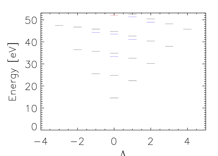
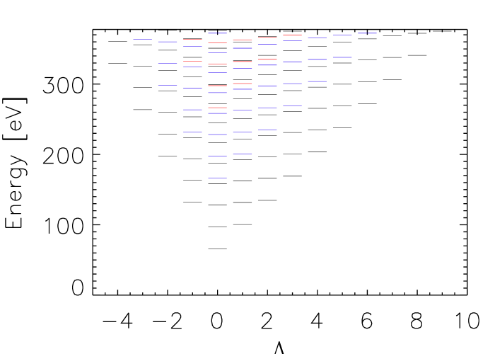
Figure 3: Rotovibrational energy spectrum ($\epsilon_{N\Lambda V}$) of He₂ in the ground state at $B=10^{12}$ G (top) and $10^{13}$ G (bottom). The zero energy corresponds to $E=-E_{m}$, while the uppermost horizontal line corresponds to $E=-E_{m}+D_{m}$ above which the molecular states become dissociated. The black, blue and red lines indicate $N=0,1$ and 2 state. For each $N$ and $\Lambda$, the horizontal lines indicate energy levels for different $V$ states.

Table 8: Number of rotovibrational states in helium molecular ions.

	$(m_{1},m_{2},m_{3},m_{4})$	$B_{12}=1$	$B_{12}=10$	$B_{12}=100$
He${}_{2}^{3+}$	(0)	0	0	1
He${}_{2}^{2+}$	(0,1)	0	8	12
	(0,2)	0	0	1
He${}_{2}^{+}$	(0,1,2)	98	177	87
	(0,1,3)	5	79	56
	(0,1,4)	0	46	42
	(0,1,5)	0	31	35
He2	(0,1,2,3)	27	132	87
	(0,1,2,4)	2	77	61
	(0,1,2,5)	0	57	52
	(0,1,2,6)	0	50	46

5 Effects of finite nuclear mass

The separation of the center-of-mass motion is non-trivial when a magnetic field is present (Herold et al., 1981). The total pseudomomentum ($\vec{K}$) is often used to take into account motional effects in a magnetic field since $\vec{K}$ is a constant of motion (Lai, 2001). In the following subsections, we discuss two effects associated with finite nuclear mass in strong magnetic fields. We denote the binding energy in the assumption of fixed nuclear location (e.g., Born-Oppenheimer approximation) as $\epsilon^{(0)}_{\kappa}(<0)$ for an electronic state $\kappa$. Since we consider states with $n=0$ and $\nu=0$, the relevant quantum numbers are $\kappa=\{m_{i}\}$ ($i$ denotes each bound electron in multi-electron atoms and molecules).

5.1 Finite nuclear mass correction

The assumption of zero transverse pseudomomentum introduces an additional term $s_{\kappa}\hbar\Omega_{B}$ in the binding energy (Herold et al., 1981; Wunner et al., 1981). $\Omega_{B}$ is the nuclear cyclotron energy and $s_{\kappa}=\sum_{i}m_{i}$ is the sum of magnetic quantum numbers for a given electronic state $\kappa$ (e.g., $s_{\kappa}=4$ for He₂ molecule in the ground state). However, the scheme assuming the zero transverse pseudomomentum does not necessarily give the lowest binding energies at $B\>\vbox{\hbox{$>$\hskip-7.5pt\lower 4.30554pt\hbox{$\sim$}}}\>B_{Q}$. Instead, LS95 and LS96 estimated lower binding energies at $B\>\vbox{\hbox{$>$\hskip-7.5pt\lower 4.30554pt\hbox{$\sim$}}}\>B_{Q}$ using another scheme which relaxed the assumption of the zero transverse pseudomomentum. A more rigorous calculation was performed for He⁺ ion by Bezchastnov et al. (1998) and Pavlov & Bezchastnov (2005). An application of such schemes to multi-electron systems is beyond the scope of this paper. We will discuss the limitation of our models at very high magnetic field in §6.

5.2 Motional Stark effects

When an atom or molecule moves across the magnetic field $\vec{B}$, a motional Stark electric field $\vec{E}_{MS}=\frac{\vec{K}\times\vec{B}}{MC}$ is induced in the center-of-mass frame. $M$ is the mass of atom or molecule. The Hamiltonian for the motional Stark field is given by

$$H_{MS}=e\frac{\vec{K}\times\vec{B}}{Mc}\vec{r}=\Omega_{B0}K_{\perp}x$$ (26)

where $\Omega_{B0}\equiv\frac{eB}{Mc}$. For a given pseudomomentum $\vec{K}$, the motional Stark field separates the guiding center of the nucleus and that of the electron by

$$R_{K}=\frac{c|\vec{K}\times\vec{B}|}{eB^{2}}=\frac{cK_{\perp}}{eB}.$$ (27)

Since the motional Stark field breaks the cylindrical symmetry preserved in magnetic field, it is non-trivial to evaluate motional Stark field effects. A non-perturbative (therefore more rigorous) approach has been applied only for one-electron systems (Vincke et al., 1992; Potekhin, 1994; Pavlov & Bezchastnov, 2005). However, such an approach is quite complicated and time-consuming especially for multi-electron atoms and molecules. Therefore, following LS95, we considered two limiting cases: (1) $R_{K}\ll\hat{\rho}$ and (2) $R_{K}\gg\hat{\rho}$ and determined general formula which can be applied to a wide range of $B$ and $K_{\perp}$. For diatomic molecules, we can apply a nearly identical scheme used for calculating transverse vibrational energy to the both cases.

5.2.1 Centered states

When the energy shift caused by motional Stark field is smaller than the spacing between binding energies, the perturbation approach is applicable (Pavlov & Meszaros (1993) and § 3.2.1). The first order perturbation energy $\langle\kappa|H_{MS}|\kappa\rangle$ vanishes since the matrix element $\langle\kappa|x|\kappa\rangle=0$. The second order perturbation energy is given by

$$\epsilon^{(2)}_{\kappa}=\sum_{\kappa^{\prime}}\frac{|\langle\kappa^{\prime}|H_{MS}|\kappa\rangle|^{2}}{\epsilon^{(0)}_{\kappa^{\prime}}-\epsilon^{(0)}_{\kappa}}=\frac{K^{2}_{\perp}}{2M}\alpha^{(2)}_{\kappa}$$ (28)

Among the various electronic states $\kappa^{\prime}=\{n^{\prime}m^{\prime}\nu^{\prime}\}$, only $n^{\prime}=0,m^{\prime}=m\pm 1,\nu^{\prime}=0$ state have non-negligible contribution to $\epsilon^{(2)}_{\kappa}$ since the other states have large $\epsilon^{(0)}_{\kappa^{\prime}}-\epsilon^{(0)}_{\kappa}$ and/or vanishing matrix element $\langle\kappa^{\prime}|x|\kappa\rangle$. Since the overlap integral of longitudinal wavefunction is close to unity (Pavlov & Meszaros, 1993), $\alpha^{(2)}_{\kappa}$ is given by

$$\alpha^{(2)}_{\kappa}\simeq\hbar\Omega_{B0}\left(\frac{m+1}{\epsilon_{m}-\epsilon_{m+1}+\hbar\Omega_{Bi}}+\frac{m}{\epsilon_{m}-\epsilon_{m-1}-\hbar\Omega_{Bi}}\right)$$ (29)

where $\epsilon_{m}=-\epsilon^{(0)}_{\kappa}(>0)$ where $m$ denotes the magnetic quantum number of the outermost electron of electronic state $\kappa$. The 2nd term is zero for the ground state. Following Pavlov & Meszaros (1993), we define the anisotropic mass $M_{\perp,\kappa}$ as

$$M_{\perp,\kappa}\equiv\frac{M}{1-\alpha^{(2)}_{\kappa}}>M.$$ (30)

The transverse energy characterized by $K_{\perp}$ is given by

$$E_{\perp,\kappa}=\frac{{K_{\perp}}^{2}}{2M_{\perp,\kappa}}.$$ (31)

The perturbation method is valid when $|\epsilon^{(2)}_{\kappa}|\ll|\Delta\epsilon^{(0)}_{\kappa}|$ (Pavlov & Meszaros, 1993) where $K_{\perp,\kappa}$ is given by

$$K_{\perp,\kappa}=\left(\frac{2M|\Delta\epsilon^{(0)}_{\kappa}|}{\alpha^{(2)}_{\kappa}}\right)^{1/2}.$$ (32)

where $|\Delta\epsilon^{(0)}_{\kappa}|$ is the spacing of the zeroth order energies (typically $|\epsilon_{m}-\epsilon_{m+1}|$).

5.2.2 Decentered states

When $R_{K}\gg\hat{\rho}$, it is convenient to utilize the so-called decentered formalism (LS95). We replace the nuclear Coulomb term by

$$V_{m}(z,R_{K})=\int{d^{2}\vec{r}_{\perp}\frac{|\Phi_{m}(\vec{r}_{\perp})|^{2}}{|\vec{r}_{\perp}+\vec{R}_{K}|}},$$ (33)

and compute binding energies at different $R_{K}$ grid points. For diatomic molecules, we replace the nuclear Coulomb term by

$$V(z,R_{K})=V_{m}\left(z-\frac{a_{0}}{2},R_{K}\right)+V_{m}\left(z+\frac{a_{0}}{2},R_{K}\right).$$ (34)

The grid calculation for $R_{K}$ is identical to the one for transverse vibrational energy in §3.2 except that the Coulomb repulsion term between two nuclei is $\frac{Z^{2}e^{2}}{a_{0}}$ (instead of $\frac{Z^{2}e^{2}}{(a^{2}_{0}+R^{2}_{K})^{1/2}}$) since motional Stark field shifts the guiding center of the two nuclei by $R_{K}$ in the transverse direction but the separation between the two nuclei is still $a_{0}$.

LS95 found that the binding energy curves are well fit by the following formula.

$$E_{\perp}(K_{\perp})+\epsilon_{\kappa}^{(0)}=-A_{1}\left(\ln\frac{1}{A_{2}+A_{3}R^{2}_{K}}\right)^{2}$$ (35)

where $A_{1},A_{2}$ and $A_{3}$ are the fit parameters. $E_{\perp}(R_{K})=E_{\perp}(K_{\perp})$ is the transverse energy and $\epsilon_{\kappa}^{(0)}$ is the binding energy in the infinite nuclear mass approximation. Figure 4 shows the binding energy curve of He₂ molecule as a function of $R_{K}$ at $B=10^{12}$ G. At small $R_{K}$, the fitted function is well matched with the results from the perturbation approach. Although mixing between different $m$ states is ignored, a comparison with Potekhin (1998) and Potekhin (1994) for hydrogen atoms indicates this approach gives better than 30% accuracy over a large range of $K_{\perp}$ (Lai & Salpeter, 1995). This is adequate for our purpose of investigating ionization and dissociation balance.

Figure 4: The transverse energy of He₂ molecule at $B=10^{12}$ G. The asterisks are the binding energies from our numerical calculation and they are fitted with the function given in (35). The dashed line shows the energy curve from the perturbation method discussed in §3.2.1 and §5.2.1.

Along with the finite nuclear mass term discussed in §5.1, the electronic energy of an atom or molecule moving with transverse pseudomomentum $K_{\perp}$ is given by

$$\epsilon_{\kappa}(K_{\perp})=\epsilon^{(0)}_{\kappa}+s_{\kappa}\hbar\Omega_{B}+E_{\perp}(K_{\perp}).$$ (36)

Note that $\epsilon^{(0)}_{\kappa}<0$ and both the second and third term decrease the binding energy. Later, we will discuss the validity of this approach at $B\>\vbox{\hbox{$>$\hskip-7.5pt\lower 4.30554pt\hbox{$\sim$}}}\>B_{Q}$.

6 Ionization and dissociation equilibrium

We have investigated the ionization and dissociation balance of magnetized helium atmospheres including the following chemical reaction channels. Table 9 and 10 list ionization and dissociation energies of various helium ions and molecular ions in the assumption with fixed nuclear location. We did not take into account the He^- ion since its ionization energy is $\la 20$ [eV] and He^- is not abundant at all in the temperature range considered here ($T\ga 10^{5}$ K).

• Ionization

  • He${}^{+}\leftrightarrow\alpha$ + e

  • He $\leftrightarrow$ He⁺ + e

  • He${}^{2+}_{2}$ $\leftrightarrow$ He${}^{3+}_{2}$ + e

  • He${}^{+}_{2}$ $\leftrightarrow$He${}^{2+}_{2}$ + e

  • He₂ $\leftrightarrow$He${}^{+}_{2}$ + e

• Dissociation

  • He${}^{3+}_{2}$ $\leftrightarrow$ $\alpha$ + He⁺

  • He${}^{2+}_{2}$ $\leftrightarrow$ $\alpha$ + He

  • He${}^{2+}_{2}$ $\leftrightarrow$ He⁺ + He⁺

  • He${}^{+}_{2}$ $\leftrightarrow$ He⁺ + He

  • He₂ $\leftrightarrow$ He + He

Table 9: Ionization energy [eV] of helium atom and molecular ions.

$B_{12}$	He+	He	He${}_{2}^{3+}$	He${}_{2}^{2+}$	He${}_{2}^{+}$	He2
1	418	159	391	418	261	137
10	847	331	885	947	603	298
100	1563	629	1833	1912	1209	643

Table 10: Dissociation energy $D_{m}$ [eV] of helium molecular ions. The numbers in the brackets are $\tilde{D}_{m}$ [eV]. The columns without a number indicate that there is no bound molecular state with respect to ions and atoms. The zero-point energy correction is not included.

$B_{12}$	He${}_{2}^{3+}$	He${}_{2}^{2+}$	He${}_{2}^{+}$	He2
1	– (–)	– (97.8)	74.6 (251)	53.1 (290)
10	37.8 (37.8)	137 (359)	410 (725)	378 (806)
100	270 (270)	619 (973)	1198 (1708)	1212 (1915)

Notes: Recent work by Turbiner & López Vieyra (2004) and Turbiner & Guevara (2006) shows He${}_{2}^{3+}$ and He${}_{2}^{2+}$ ion can exist at $B\ga(2.4-2.6)\times 10^{12}$ G. Our results are roughly consistent with theirs.

The Saha-Boltzmann equation for ionization balance is given as,

$$\frac{n_{i}}{n_{i+1}n_{e}} = \frac{z_{i}}{z_{i+1}z_{e}}$$ (37)

where $z_{e}$ is the partition function for an electron,

$$z_{e}=2\left(\frac{m_{e}kT}{2\pi\hbar^{2}}\right)^{3/2}\frac{\eta_{e}}{\tanh{\eta_{e}}},$$ (38)

$\eta_{e}=\hbar\omega_{B}/2kT$ and $\omega_{B}=eB/m_{e}c$ is the electron cyclotron frequency (Gnedin et al., 1974). The quantity $z_{i}$ is the partition function for ionization state $i$,

$$z_{i}=\left(\frac{M_{i}kT}{2\pi\hbar^{2}}\right)^{1/2}\frac{\eta_{i}}{\sinh{\eta_{i}}}\int_{0}^{\infty}\frac{K_{\perp}dK_{\perp}}{2\pi\hbar^{2}}\sum_{\kappa}w_{i,\kappa}(K_{\perp})\exp{\left(-\frac{\epsilon_{i,\kappa}(K_{\perp})}{kT}\right)}$$ (39)

where $E_{i}$, $Z_{i}$ and $M_{i}$ are the ground state energy, the charge and the mass of an ion $i$. $\eta_{i}=\hbar\Omega_{Bi}/2kT$ where $\Omega_{Bi}=Z_{i}eB/M_{i}c$ is the ion cyclotron frequency. $\epsilon_{i,\kappa}(K_{\perp})(<0)$ is the binding energy of a bound state $\kappa$ given in equation (36). $w_{i,\kappa}$ is the occupation probability. In general, $w_{i,\kappa}(K_{\perp})$ is a function of $Z_{i}$, $Z_{p}$ (the charge of perturbing ions, usually the effective charge of the plasma), $\epsilon_{i,\kappa}(K_{\perp})$ and $\rho$ (the plasma density). $w$ depends not only on the type of ion $i$, the electronic state $\kappa$ and the transverse pseudomomentum $K_{\perp}$, but also it is different for each bound electron. Obviously, electrons in the outer shells are subject to a stronger electric field from neighboring ions than those in the inner shells. We explicitly computed $w_{i,\kappa}$ for all the bound electrons using the electronic microfield distribution of Potekhin et al. (2002).

The Saha-Boltzmann equation for dissociation balance is given as

$$\frac{n_{j}}{n_{k}n_{l}} = \frac{\tilde{z}_{j}}{z_{k}z_{l}}$$ (40)

where $\tilde{z}_{j}$ is the partition function for molecular ionization state $j$,

$$\tilde{z}_{j} = \displaystyle\left(\frac{M_{j}kT}{2\pi\hbar^{2}}\right)^{1/2}\frac{\eta_{j}}{\sinh{\eta_{j}}}\int_{0}^{\infty}\frac{K_{\perp}dK_{\perp}}{2\pi\hbar^{2}}\sum_{\kappa}w_{j,\kappa}(K_{\perp})$$ (41)

$$\times\exp{\left(-\frac{\epsilon_{j,\kappa}(K_{\perp})}{kT}\right)}\sum_{N,\Lambda,V}^{\epsilon_{N\Lambda V}<D_{\kappa}}\exp{\left(-\frac{\epsilon_{N\Lambda V}}{kT}\right)}$$

where $E_{j}$, $Z_{j}$ and $M_{j}$ are the ground state energy, the charge and the mass of a molecular ion $j$. $\eta_{j}=\hbar\Omega_{Bj}/2kT$ where $\Omega_{Bj}=Z_{j}eB/M_{j}c$ is the molecular ion cyclotron frequency. $\epsilon_{j,\kappa}(K_{\perp})(<0)$ and $w_{j,\kappa}(K_{\perp})$ are the binding energy and occupation probability of an electronic bound state $\kappa$. $\epsilon_{N\Lambda M}(>0)$ is the excitation energy of a rotovibrational state $(N,\Lambda,V)$. We took the summation $\sum_{N,\Lambda,V}$ until $\epsilon_{N\Lambda V}$ exceeds the dissociation energy $D_{\kappa}$. The set of the Saha-Boltzmann equations along with the condition for the baryon number conservation and charge neutrality are iteratively solved until we reached sufficient convergence in $\Delta n_{e}/n_{e}$ ($<10^{-6}$) where $n_{e}$ is the density of free electrons. The convergence was achieved rapidly in most cases (less than 10 iterations were required).

Figure 5, 6 and 7 show the fraction of helium ions and molecular ions at $B=10^{12},10^{13}$ and $10^{14}$ G. At $B=10^{12}$ G, He${}_{2}^{3+}$ and He${}_{2}^{2+}$ are not present because they are not bound with respect to their dissociated atoms and ions (table 10). In all the cases, the He${}_{2}^{3+}$ fraction is negligible because helium molecular ions with more electrons have much larger binding energies. At $B=10^{14}$ G, He₂ is not present because even the ground state becomes auto-ionized to He${}_{2}^{+}$ ion due to the finite nuclear mass effect although He₂ remains bound with respect to two helium atoms. Note that the ionization energy of He₂ at $10^{14}$ G is 643 eV (table 9) while the difference in the energy due to the finite nuclear mass term between He₂ and He${}_{2}^{+}$ is 945 eV. As discussed in §5.1, our scheme using the zero pseudomomentum becomes invalid at $B\>\vbox{\hbox{$>$\hskip-7.5pt\lower 4.30554pt\hbox{$\sim$}}}\>B_{Q}$ and in reality He₂ will have lower binding energy than He${}^{+}_{2}$. Therefore, our results at $B=10^{14}$ G should be taken with caution. Figure 8 shows the temperature dependence of the helium atomic and molecular fractions at different B-field strengths. We fixed the plasma density to the typical density of the X-mode photosphere ($\sim 10,10^{2}$ and $10^{3}$ g/cm³ for $B=10^{12},10^{13}$ and $10^{14}$ G (Lai & Salpeter, 1997)). The transition from molecules to helium atoms and ions takes place rapidly at $T\sim 3\times 10^{5}$ K and $\sim 6\times 10^{5}$ K for $B=10^{12}$ G and $10^{13}$ G.

Figure 5: Ionization and dissociation balance of helium at $T=10^{5.5}$ K (top) and $10^{6}$ K (bottom) at $B=10^{12}$ G.

Figure 6: Ionization and dissociation balance of helium at $T=10^{5.5}$ K (top) and $T=10^{6}$ K (bottom) at $B=10^{13}$ G.

Figure 7: Ionization and dissociation balance of helium at $T=10^{5.5}$ K (top) and $T=10^{6}$ K (bottom) at $B=10^{14}$ G.

Figure 8: Temperature dependence of helium atomic and molecular fraction at $B=10^{12}$ G ($\rho=10$ g/cm³), $B=10^{13}$ G ($\rho=10^{2}$ g/cm³) and $B=10^{14}$ G ($\rho=10^{3}$ g/cm³).

In order to illustrate different physical effects, we show the fraction of helium atoms and He₂ molecules as a function of temperature in Figure 9. When motional Stark effects are ignored (dotted line), the molecular fraction is underestimated because helium ions and atoms are subject to a larger motional Stark field due to their smaller masses and binding energies. As expected, molecules become more abundant when rotovibrational states are included. The discrepancy from the results without rotovibrational states (dashed line) increases toward higher temperature since more rotovibrational states have larger statistical weight as their excitation energies are an order of 100 eV at $B=10^{13}$ G (see figure 3). When we take into account only the ground states (dot-dashed line), the results are close to the case without motional Stark effects because the ground states are less affected by motional Stark effects than the excited states.

Figure 9: Fraction of helium atoms (left) and helium molecules (right) $\rho=10^{2}$ g/cm³ at $B=10^{13}$ G. The solid lines show the results by taking into account all the physical effects discussed in this paper. The dotted and dashed lines ignored motional Stark effects and rotovibrational states respectively. The dot-dashed lines include only the ground states.

6.1 He₃ molecule and larger helium molecular chains

When He₂ is abundant, larger helium molecules such as He₃ may become abundant. We roughly estimated the fraction of He₃ molecules by neglecting the finite nuclear mass effects and zero-point vibrational energy correction both of which will reduce the dissociation energy. Similarly to He₂, we computed the binding energy of He₃ molecules by Hartree-Fock calculation. The dissociation energy of He${}_{3}\rightarrow$He₂+He is 289 and 1458 eV at $B=10^{13}$ and $10^{14}$ G. Our results are close to those of the density functional calculation by ML06 (384 and 1647 [eV] at $B=10^{13}$ and $10^{14}$ G). Note that the density function calculation overestimates binding energies by $\sim 10$% compared with more accurate Hartree-Fock calculation (ML06). Assuming the internal degrees of freedom are similar between He₂ and He₃ molecule and neglecting the bending degree of freedom for He₃, we computed dissociation equilibrium between He₂ and He₃ following Lai & Salpeter (1997).

Figure 10 shows contours of the He₃ molecule fraction with respect to He₂ molecule at $B=10^{13}$ G. In the dotted area, the fraction of diatomic helium molecular ions is larger than 10%. It is seen that He₃ molecule will be abundant at $T\la 3\times 10^{5}$ K at $B=10^{13}$ G. The results are consistent with the estimates of molecular chain formation by Lai (2001) and ML06. ML06 provided binding energy of infinite He molecular chain as $E_{\infty}\simeq 1.25B^{0.38}_{13}$ keV at $B\ga 10^{13}$ G. From this fitting formula, the cohesive energy of helium molecular chains is given as $E_{co}\sim 0.36,1.5$ and 5.1 keV at $B=10^{13},10^{14}$ and $10^{15}$ G. When $kT\la 0.1E_{co}$, molecular chains are likely to be formed (Lai, 2001); consequently, we expect helium molecular chains to form at $T\la 3\times 10^{5},1\times 10^{6}$ and $5\times 10^{6}$ K and $B\ga 10^{13},10^{14}$ and $10^{15}$ G.

Figure 10: Ratio of He₃ with respect to He₂ at $B=10^{13}$ G (solid curve contours). The dotted area shows the $(\rho,T)$ regime where a fraction of diatomic helium molecular ions is larger than 10%.

7 Application

We investigated the ionization and dissociation balance of helium atmospheres for two classes of INS whose X-ray spectra show absorption features.

7.1 Radio-quiet neutron stars

A class of INS called radio-quiet neutron stars (RQNS) is characterized by their X-ray thermal spectra with $T\la 10^{6}$ K and spin-down dipole B-field strength $B\ga 10^{13}$ G. A single or multiple absorption features have been detected from six radio-quiet NS (Haberl et al., 2003, 2004; van Kerkwijk et al., 2004). Although the interpretation of these features is still in debate, helium is certainly one of the candidates for the surface composition of RQNS (van Kerkwijk & Kaplan, 2006). Timing analysis suggests that a couple of RQNS have dipole magnetic field strengths in the range of $B=10^{13}$–$10^{14}$ G (Kaplan & van Kerkwijk, 2005). Therefore, we investigated the ionization/dissociation balance of a helium atmosphere at $B=3\times 10^{13}$ G. Figure 11 shows the contours of He⁺ and He molecular fractions at $3\times 10^{13}$ G. He⁺ is dominant at $T\sim 10^{6}$ K and molecules become largely populated at $T\la 5\times 10^{5}$ K.

Suppose all the RQNS have helium atmospheres on the surface. RQNS with higher temperatures ($T\sim 10^{6}$ K) such as RXJ0720.4-3125 and RXJ1605.3+3249 will have He⁺ ions predominantly with a small fraction of He atoms. Indeed, several bound-bound transition lines of He⁺ ion have energies at the observed absorption line location at $B\ga 10^{13}$ G (Pavlov & Bezchastnov, 2005). On the other hand, RQNS with lower temperatures ($T\sim 5\times 10^{5}$ K) such as RXJ0420.0-5022 may have some fraction of helium molecules, although the He⁺ ion is still predominant at low densities where absorption lines are likely formed.

Figure 11: Ionization and dissociation balance of helium at $B=3\times 10^{13}$ G. The dotted area is where the fraction of helium molecules and molecular ions (including He₂, He${}_{2}^{+}$, He${}_{2}^{2+}$ and He${}_{2}^{3+}$) becomes more than 50%. The black area is where the fraction of He⁺ becomes more than 50%. The white region on the right is where the fraction of bare helium ions becomes more than 50%. In the narrow white region betweeen the dotted and black area, atomic helium is somewhat abundant, so neither molecular nor singly ionized helium dominates.

7.2 1E1207.4-5209

1E1207.4-5209 is a hot isolated NS with age $\sim 7\times 10^{3}$ yrs. The fitted blackbody temperature is $\sim 2\times 10^{6}$ K (Mori et al., 2005). Presence of a non-hydrogenic atmosphere has been suggested since 1E1207 shows multiple absorption features at higher energies than hydrogen atmosphere models predicted (Sanwal et al., 2002; Hailey & Mori, 2002; Pavlov & Bezchastnov, 2005; Mori & Hailey, 2006). Sanwal et al. (2002) interpreted the observed features as bound-bound transition lines of a He⁺ ion at $B=2\times 10^{14}$ G. Also, Turbiner (2005) suggested that He${}^{3+}_{2}$ molecular ion may be responsible for one of the absorption features observed in 1E1207 at $B\sim 4.4\times 10^{13}$ G.

However, our study shows that the fraction of He${}^{3+}_{2}$ molecular ions is negligible at any B-field and temperature because more neutral molecular ions have significantly larger binding energies. We also investigated ionization/dissociation balance of helium atmospheres at $2\times 10^{14}$ G (figure 12). At $B\>\vbox{\hbox{$>$\hskip-7.5pt\lower 4.30554pt\hbox{$\sim$}}}\>B_{Q}$, our scheme of treating finite nuclear mass effects becomes progressively inaccurate. As a result, the ionization energy of helium atoms becomes significantly smaller and the He₂ molecule becomes auto-ionized due to the finite nuclear mass correction discussed in §5.1. Therefore, the molecular fraction will be underestimated in this case (the left panel in figure 12). On the other hand, when we ignore the finite nuclear mass effects (the right panel in figure 12), the molecular fraction is likely overestimated. We expect that a realistic ionic and molecular fraction will be somewhere between the two cases. It is premature to conclude whether He⁺ is dominant for the case of 1E1207 since we do not have a self-consistent temperature and density profile. The study of ML06 and Lai (2001) also suggests the critical temperature below which helium molecule chains form is $\sim 2\times 10^{6}$ K at $B=2\times 10^{14}$ G. This is close to the blackbody temperature of 1E1207. Further detailed studies are necessary to conclude the composition of helium atmospheres at $B=2\times 10^{14}$ G.

Figure 12: Ionization and dissociation balance of helium at $B=2\times 10^{14}$ G. The top and bottom figure show the results with and without the finite nuclear mass effects respectively. In the dotted region the molecular and molecular ion fraction exceeds one half. In the black region singly ionized atomic helium dominates, and the white region demarcates fully ionized helium.

8 Discussion

We have examined the ionization-dissociation balance of the helium atmospheres of strongly magnetized neutron stars. As the observational data on isolated neutron stars has improved over the past decade (Sanwal et al., 2002; Hailey & Mori, 2002; van Kerkwijk & Kaplan, 2006), both hydrogen and iron atmospheres have lost favour, and atmospheres composed of other elements have been invoked to interpret both the continuum and spectral properties of neutron stars. On the other hand the theoretical investigations of Chang et al. (2004) and Chang & Bildsten (2004) have shown that diffusive nuclear burning may quickly deplete the hydrogen by so the NS surface may be composed of helium or heavier elements.

The results found here indicate several avenues for future work. Although the treatment of finite nuclear mass effects is problematic in the strong field limit, only by including this accurately can we know the physical state of matter in super-critical magnetic fields – solid, liquid or gas. The state can have significant effects of the outgoing radiation from these objects. It is also important to repeat a similar calculation to that presented here for molecular chains, including all of the relevant degrees of freedom of the chains, i.e. including the bending modes which were neglected here. Regardless, the high abundance of molecules under the conditions of observed neutron star atmospheres is bound to spur additional research into the statistical mechanics of highly magnetized molecules and polymers.

At the temperatures and densities of neutron star atmospheres the rotovibrational excitations of helium molecules are populated. Including these excitations increases the expected abundance of molecules by up to two orders of magnitude relative to calculations that ignore the internal states of the molecule. Ionization, dissociation and electric excitation energies of helium molecules are larger than 100 eV at $B\>\vbox{\hbox{$>$\hskip-7.5pt\lower 4.30554pt\hbox{$\sim$}}}\>10^{13}$ G. On the other hand, rotovibrational excitation energies are in the range of 10–100 eV at $B=10^{12}$–$10^{14}$ G. If helium molecules are abundannt, their spectroscopic signatures may be detected in the optical, UV and X-ray band. If helium comprises the atmospheres of isolated neutron stars, clearly it is crucial to understand the structure of helium molecules and molecular chains in order to interpret the spectra from neutron stars.

References

- Alcock & Illarionov (1980) Alcock, C. & Illarionov, A. 1980, ApJ, 235, 534
- Bezchastnov et al. (1998) Bezchastnov, V. G., Pavlov, G. G., & Ventura, J. 1998, Phys. Rev. A, 58, 180
- Chang et al. (2004) Chang, P., Arras, P., & Bildsten, L. 2004, ApJL, 616, L147
- Chang & Bildsten (2004) Chang, P. & Bildsten, L. 2004, ApJ, 605, 830
- Demeur et al. (1994) Demeur, M., Heenen, P. ., & Godefroid, M. 1994, Phys. Rev. A, 49, 176
- Gnedin et al. (1974) Gnedin, Y. N., Pavlov, G. G., & Tsygan, A. I. 1974, Soviet Physics JETP, 39, 201
- Haberl et al. (2003) Haberl, F., Schwope, A. D., Hambaryan, V., Hasinger, G., & Motch, C. 2003, A&A, 403, L19
- Haberl et al. (2004) Haberl, F., Zavlin, V. E., Trümper, J., & Burwitz, V. 2004, A&A, 419, 1077
- Hailey & Mori (2002) Hailey, C. J. & Mori, K. 2002, ApJL, 578, L133
- Herold et al. (1981) Herold, H., Ruder, H., & Wunner, G. 1981, Journal of Physics B Atomic Molecular Physics, 14, 751
- Kaplan & van Kerkwijk (2005) Kaplan, D. L. & van Kerkwijk, M. H. 2005, ApJ, 635, L65
- Khersonskii (1984) Khersonskii, V. K. 1984, AP&SS, 98, 255
- Khersonskii (1985) —. 1985, Ap&SS, 117, 47
- Lai (2001) Lai, D. 2001, Rev. Mod. Phys., 73, 629
- Lai & Salpeter (1995) Lai, D. & Salpeter, E. E. 1995, Phys. Rev. A, 52, 2611
- Lai & Salpeter (1996) —. 1996, Phys. Rev. A, 53, 152
- Lai & Salpeter (1997) —. 1997, ApJ, 491, 270
- Lai et al. (1992) Lai, D., Salpeter, E. E., & Shapiro, S. L. 1992, Phys. Rev. A, 45, 4832
- Medin & Lai (2006a) Medin, Z. & Lai, D. 2006a, submitted to Phys. Rev. A (astro-ph/0607166)
- Medin & Lai (2006b) —. 2006b, submitted to Phys. Rev. A (astro-ph/0607277)
- Mori et al. (2005) Mori, K., Chonko, J. C., & Hailey, C. J. 2005, ApJ, 631, 1082
- Mori & Hailey (2002) Mori, K. & Hailey, C. J. 2002, ApJ, 564, 914
- Mori & Hailey (2006) —. 2006, ApJ, 648, 1139
- Morse (1929) Morse, P. M. 1929, Physical Review, 34, 57
- Neuhauser et al. (1987) Neuhauser, D., Koonin, S. E., & Langanke, K. 1987, Phys. Rev. A, 36, 4163
- Pavlov & Bezchastnov (2005) Pavlov, G. G. & Bezchastnov, V. G. 2005, ApJL, 635, L61
- Pavlov & Meszaros (1993) Pavlov, G. G. & Meszaros, P. 1993, ApJ, 416, 752
- Potekhin (1994) Potekhin, A. Y. 1994, J. Phys. B, 27, 1073
- Potekhin (1998) —. 1998, J. Phys. B, 31, 49
- Potekhin et al. (2002) Potekhin, A. Y., Chabrier, G., & Gilles, D. 2002, Phys. Rev. E, 65, 36412
- Romani (1987) Romani, R. W. 1987, ApJ, 313, 718
- Sanwal et al. (2002) Sanwal, D., Pavlov, G. G., Zavlin, V. E., & Teter, M. A. 2002, ApJL, 574, L61
- Turbiner (2005) Turbiner, A. V. 2005, preprint (astro-ph/0506677)
- Turbiner & Guevara (2006) Turbiner, A. V. & Guevara, N. L. 2006, preprint (astro-ph/0610928)
- Turbiner & López Vieyra (2004) Turbiner, A. V. & López Vieyra, J. C. 2004, preprint (astro-ph/0412399)
- Turbiner & López Vieyra (2003) Turbiner, A. V. & López Vieyra, J. C. 2003, Phys. Rev. A, 68, 012504
- van Kerkwijk & Kaplan (2006) van Kerkwijk, M. H. & Kaplan, D. L. 2006, to appear in Astrophysics and Space Science, in the proceedings of ”Isolated Neutron Stars: from the Interior to the Surface”, edited by D. Page, R. Turolla and S. Zane, preprint (astro-ph/0607320)
- van Kerkwijk et al. (2004) van Kerkwijk, M. H., Kaplan, D. L., Durant, M., Kulkarni, S. R., & Paerels, F. 2004, ApJ, 608, 432
- Vincke et al. (1992) Vincke, M., LeDourneuf, M., & Baye, D. 1992, Journal of Physics B Atomic Molecular Physics, 25, 2787
- Woods et al. (2006) Woods, P. M., Zavlin, V. E., & Pavlov, G. G. 2006, to appear in Astrophysics and Space Science, in the proceedings of ”Isolated Neutron Stars: from the Interior to the Surface”, edited by D. Page, R. Turolla and S. Zane, preprint (astro-ph/0608483)
- Wunner et al. (1981) Wunner, G., Ruder, H., & Herold, H. 1981, ApJ, 247, 374