Colour-colour diagrams and extragalactic globular cluster ages

Abstract

Context. Age and metallicity estimates for extragalactic globular clusters, from integrated colour-colour diagrams, are examined.

Aims. We investigate biases in cluster ages and [Fe/H] estimated from the $(V-K)-(V-I)$ diagram, arising from inconsistent Horizontal Branch morphology, metal mixture, treatment of core convection between observed clusters and the theoretical colour grid employed for age and metallicity determinations. We also study the role played by statistical fluctuations of the observed colours, caused by the low total mass of typical globulars.

Methods. Synthetic samples of globular cluster systems are created, by means of Monte-Carlo techniques. Each sample accounts for a different possible source of bias, among the ones addressed in this investigation. Cumulative age and [Fe/H] distributions are then retrieved by comparisons with a reference theoretical colour-colour grid, and analyzed.

Results. Horizontal Branch morphology is potentially the largest source of uncertainty. A single-age system harbouring a large fraction of clusters with an HB morphology systematically bluer than the one accounted for in the theoretical colour grid, can simulate a bimodal population with an age difference as large as $\sim$8 Gyr. When only the redder clusters are considered, this uncertainty is almost negligible, unless there is an extreme mass loss along the Red Giant Branch phase. The metal mixture affects mainly the redder clusters; the effect of colour fluctuations becomes negligible for the redder clusters, or when the integrated $M_{V}$ is brighter than $\sim-$8.5 mag. The treatment of core convection is relevant for ages below $\sim$4 Gyr. The retrieved cumulative [Fe/H] distributions are overall only mildly affected. Colour fluctuations and convective core extension have the largest effect. When 1$\sigma$ photometric errors reach 0.10 mag, all biases found in our analysis are erased, and bimodal age populations with age differences of up to $\sim$8 Gyr go undetected. The use of both $(U-I)-(V-K)$ and $(V-I)-(V-K)$ diagrams may help disclosing the presence of blue HB stars unaccounted for in the theoretical colour calibration.

1 Introduction

A large number of studies about extragalactic globular cluster (GC) systems has appeared in the last decades (see, e.g. the reviews by Ashman & Zepf az98 (1998) and Brodie & Strader bs06 (2006)). The main motivation for these analyses is that GCs are expected to be good tracers of major episodes of star formation of spheroids (see, e.g., Schweitzer sch97 (1997); Kissler-Patig, Forbes & Minniti kpfm98 (1998)) and in fact inferred GC age/metallicity distributions have been widely used to investigate the formation and evolution histories of early-type galaxies (see, e.g., Kuntschner et al. kz02 (2002); Larsen et al. lar03 (2003); Strader & Brodie  sb04 (2004); Yi et al. yi04 (2004); Hempel et al. hem05 (2005) and references therein). One of the most relevant discoveries in the field is the fact that most (if not all) extragalactic GC systems show a (integrated) colour bimodality (see, e.g., Gebhardt & Kissler-Patig gkp99 (1999)) indicating two distinct GC subpopulations, that is, two major star-forming episodes or at least two different formation mechanisms in the galaxy evolution histories (see Yoon et al. yo06 (2006) for an alternative view on this issue).

The interpretation of this bimodality in terms of age and/or chemical composition differences is complicated by the well known age-metallicity degeneracy (e.g. Worthey w94 (1994)) whereby the effect on the integrated colours of an age increase at fixed metallicity, can be reproduced also by suitably increasing the metallicity while keeping the age fixed. The age-metallicity degeneracy can be broken in a number of ways. The first one is to employ spectroscopic absorption feature indices, like the Lick/IDS ones (Burstein et al. bur84 (1984); Trager et al. trag98 (1998)). Balmer line indices are strongly sensitive to the population age, whereas metal line indices provide estimates of the GC chemical composition (see, e.g., Beasley et al. bea00 (2000); Strader et al. stra05 (2005) and reference therein for examples of application of these indices to the study of extragalactic GCs). A second possibility is to use suitable broad-band colour-colour diagrams, whereby one of the two colours is more sensitive to the age of the population, and the other is more affected by the metallicity. A widely used diagram is $(V-I)-(V-K)$ (see, e.g., Hempel et al. hem03 (2003); Hempel & Kissler-Patig hem04 (2004); Larsen, Brodie & Strader  lar05 (2005)) but there are also other possible colour combinations, that include at least one near-IR filter as summarized and discussed in James et al. (jam06 (2006)) – see also Rejkuba (rej01 (2001)) and Hempel et al. (hem05 (2005)). In addition, the $(U-B)-(B-V)$ diagram can in principle also be used to disentangle age and metallicity effects in case of old populations (see, e.g., Yi et al. yi04 (2004) for an application to the GCs of NGC 5128). A third possibility to break the age-metallicity degeneracy is to fit the observed spectral energy distribution (SED) of the cluster – where SED denotes in this case an ensemble of absolute magnitudes in a given set of broad-band filters – as discussed by Anders et al. (and04 (2004)) and De Grijs et al. (degr05 (2005); see also Fan et al. fan06 (2006)). In these papers the authors consider broad-band filters ranging from $U$ to $H$, and show how a SED composed of the $BVIH$ or $UBVI$ filters is best suited to break the degeneracy in the GC age regime.

The most accepted view about the observed GC colour bimodality is that it is driven mainly by metallicity (but see also Yoon et al. yo06 (2006) for an alternative explanation based on the morphology of the clusters’ Horizontal Branch) with the blue subpopulation being the metal poorer one. The age distribution of these two subpopulations is however still a matter of debate. As reviewed in detail by Brodie & Strader (bs06 (2006)) the metal poor GCs are generally considered to be old, of age comparable to the age of the universe and of the oldest Galactic GCs, whereas conflicting results are obtained for the metal rich ones. A representative case of this uncertainty is the GC system of NGC 4365, recently reanalyzed in detail by Larsen et al. (lar05 (2005)). The authors discuss how different datasets of absorption feature indices give contradictory results about the presence of a metal rich young GC component; also broad-band colours provide conflicting results, due to offsets between photometries, between theoretical integrated colours obtained from different authors, and possible offsets between observed Galactic GC colours (especially $(V-K)$) and the theoretical counterparts.

A definitive conclusion about the existence of a young component in extragalactic GC systems is important to constrain scenarios for the formation of spheroids. Necessary steps in this direction involve detailed assessments of systematic uncertainties related to the age determination methods using absorption feature indices and integrated magnitudes and colours. Here we will address methods based on integrated colour-colour diagrams.

A general analysis (although not specialized to the estimate of GC ages) about uncertainties in theoretical integrated colours of single age/single metallicity populations (also denoted as Simple Stellar Populations – SSPs) was published by Charlot, Worthey & Bressan (cwb96 (1996)) who compared results obtained from different sets of stellar models and different spectral libraries. More recently Yi (yi03 (2003)) discussed in a systematic way the effect of some theoretical uncertainties on selected SSP synthetic colours. Lamers, Anders & de Grijs (lam06 (2006)) have investigated the effect on the photometric evolution of unresolved star clusters (for the case of solar metallicity) of preferential loss of low mass stars from a GC, due to mass segregation and evaporation. This process may alter appreciably the integrated colours of GCs.

In this paper we focus specifically on the $(V-I)-(V-K)$ diagram used in many studies of extragalactic GCs, like the NGC 4365 system that – as already mentioned – provides conflicting results about the cluster age distribution. In particular, we analyze theoretically the effect of a number of systematic uncertainties, on both the inferred cumulative age distribution and the [Fe/H] cumulative distribution. This follows the works by, e.g., Hempel et al. (hem03 (2003)) and Hempel & Kissler-Patig (hem04 (2004)) that show how the use of the cumulative age distribution provides a powerful tool to establish the presence of a young GC subpopulation. These authors discussed in detail the effect of the GC sample size, observational effects due to contamination by background objects, and the use of different population synthesis models. To push further the analysis of this method, we investigate systematic effects related to the morphology of the Horizontal Branch (HB) that cannot be reliably predicted by theory yet; the metal mixture of the stars harboured by the observed GCs (that cannot be inferred from the colour-colour diagram only); the possible efficiency of overshooting from the convective cores (when present) and statistical colour fluctuations caused by the undersampling of the bright and fast evolutionary phases (RGB, Asymptotic Giant Branch) due to the low total mass of GCs. Our analysis is done differentially, with respect to reference synthetic samples, and makes use of our own stellar population synthesis database (the BaSTI database, see Pietrinferni et al. pietr04 (2004), pietr06 (2006)). We want to establish, in particular, if the effects we examine are able to mimic a bimodal-age distribution, even in case of a constant age for the whole cluster population. We also wish to assess eventual biases in the cluster metallicity distribution inferred from the colour-colour diagram, given the importance of determining both age and metallicity distributions of GC systems to probe the formation histories of the parent galaxies.

The next section presents briefly the theoretical population synthesis models used in our analysis, and discusses the determination of integrated magnitudes and colours. Section 3 describes the method of construction of template GC samples used as reference for our differential study, and Section 4 presents a quantitative analysis of the sources of systematic uncertainties listed above. A summary and conclusions follow in Section 5. The Appendix provides useful analytical relationships to determine the cumulative age distribution of a sample of GCs from their $(V-K)-(V-I)$ colours, and a test for the accuracy of our theoretical colour calibrations.

2 Stellar model database and computation of integrated magnitudes/colours

The stellar population model database adopted in our analysis is the so-called BaSTI (a Bag of Stellar Tracks and Isochrones) that can be accessed on the web at the official site: http://www.te.astro.it/BASTI/index.php. A description of the database can be found at the website as well as in Pietrinferni et al. (pietr04 (2004), pietr06 (2006)) and Cordier et al. (cpc06 (2006)). The stellar model/isochrone part of the database covers 11 different metallicities (from extreme Pop II stars to super metal rich populations) and two different heavy element mixtures for each metallicity, i.e. scaled solar and $\alpha$-enhanced typical of the Galactic halo population. We employed consistent bolometric corrections for both scaled-solar and $\alpha-$enhanced mixtures, even at super-solar metallicities. The evolutionary tracks follow all major stages until the end of the Asymptotic Giant Branch (AGB) or carbon ignition, depending on the value of the stellar mass. Mass loss from the stellar surface is accounted for using the Reimers (rei75 (1975)) law and two values of the free parameter $\eta$ ($\eta$=0.2 and 0.4, respectively). Superwinds along the AGB phases are also accounted for. In case of stars that develop convective cores during the central H-burning phase we have computed models with and without overshoot from the Schwarzschild boundary of the central convective regions.

We have determined the integrated magnitudes (and colours) presented in this work as follows. When analytical integrated magnitudes for an SSP with a given age $t$ and metallicity $Z$ are needed, we simply integrate the flux in the chosen filters along the representative isochrone; we employ the Initial Mass Function (IMF) by Kroupa, Tout & Gilmore (ktg93 (1993)) to determine the number of objects populating each point along the isochrone, and an appropriately chosen normalization constant. The upper mass limit is given by the most massive star still evolving along the isochrone, the lower mass limit is equal to 0.5 $M_{\odot}$, that is the lower mass limit of the models in the BaSTI database. Objects with masses below this limit contribute only negligibly to the integrated magnitudes and colours we are dealing with, as we have verified by implementing the very low mass star models by Cassisi et al. (cas00 (2000)), that extend down to $\sim$0.1$M_{\odot}$. The value of the IMF normalization constant appropriate for the specified total mass $M_{t}$ is obtained by enforcing the condition $M_{t}=\int_{M_{l}}^{M_{u}}\psi(M)MdM$ where $\psi(M)$ is the IMF, $M$ is the stellar mass, $M_{l}$ and $M_{u}$ the lower and upper mass values set, respectively, to 0.1$M_{\odot}$ (the contribution to the total cluster mass of objects with masses below 0.5 $M_{\odot}$ cannot be neglected) and to the highest stellar mass still evolving in a population of that age and $Z$. The resulting analytical integrated colours are independent of the total cluster mass $M_{t}$. Whenever integrated magnitudes and colours are needed for a ($t$, $Z$) combination not available in the isochrone database, they are determined by quadratic interpolation within our ($t$, $Z$) grid.

The analytical computation described above is somewhat the standard procedure followed in the literature. However, this procedure is strictly valid only when the number of stars is formally infinite. Whereas the analytical computation implies that all points along the isochrones are smoothly populated by a number of stars that can be equal to just a fraction of unity in case of fast evolutionary phases, in real clusters the number of objects at a point along the Colour Magnitude Diagram (CMD) is either zero or a multiple of unity. When the number of stars harboured by the observed population is not large enough to sample smoothly all evolutionary phases, statistical fluctuations of star counts will arise. This means that an ensemble of SSPs all with the same $M_{t}$, $t$ and $Z$ will show a range of integrated magnitudes (and colours) due to stochastic variations of the number of objects populating the faster evolutionary phases, that in case of intermediate/old SSPs are the upper RGB and AGB. The magnitude of these fluctuations will be larger in the wavelength ranges most affected by the flux emitted by RGB and AGB stars, typically the near-IR and longer wavelengths. This is the origin of the colour statistical fluctuations we will discuss in the next section, and that have been addressed in the literature by, e.g., Chiosi, Bertelli & Bressan (cbb88 (1988)), Girardi & Bica (gb93 (1993)), Santos & Frogel (sf97 (1997)), Cerviño & Valls-Gabaud (cer03 (2003)), Cerviño & Luridiana (cl04 (2004)), Fagiolini, Raimondo & Degl’Innocenti (frd06 (2006)).

To take into account the effect of these fluctuations we have computed integrated magnitudes and colours with a Monte-Carlo formalism. For a selected pair ($t$, $Z$) we have first determined the appropriate isochrone by interpolating quadratically (when necessary) in both age and metallicity among a set of BaSTI isochrones. As a next step, star masses are randomly extracted following the Kroupa et al. (ktg93 (1993)) IMF, until a specified value of $M_{t}$ is reached. The position of the individual stars along the isochrone is determined by linear interpolation between the two neighbouring tabulated mass values (a linear interpolation is sufficient, given the large number of points – 2250 – used to sample the isochrone). The fluxes of all synthetic stars populating the isochrone are then added, and magnitudes plus colours computed.

As a technical detail, we add that to compute the value of the SSP mass consistently with the analytical procedure, the lower limit for the random extraction of stellar masses is set to 0.1$M_{\odot}$. Whenever a mass value between this limit and 0.5$M_{\odot}$ is extracted, it is added to the total mass budget but disregarded for the isochrone population.

3 Reference GC populations

As stated in the Introduction, the aim of this paper is to investigate the effect of a number of systematic uncertainties on GC age and [Fe/H] cumulative distributions, as inferred from the integrated $(V-I)-(V-K)$ diagram. As a first step we need to create some reference GC population that will be used for differential comparisons. We have therefore first created a synthetic GC system (labelled ’template’ system) with the following characteristics:

• We employed $\alpha$-enhanced isochrones (with a mean [$\alpha$/Fe]$\sim$0.4, the exact individual abundances of the metal distribution are listed in Pietrinferni et al. pietr06 (2006)) without overshooting beyond the Main Sequence convective core boundaries (for the appropriate mass range) and mass loss parameter $\eta$=0.2 constant for all RGB stars. The HB part of the isochrone is a clump of stars, because of the constant value of $\eta$. This is fairly typical of the isochrones used in population synthesis modelling (see, e.g., Girardi et al. g00 (2000)).

• The individual GC total masses ($M_{t}$) follow the McLaughlin (mcl94 (1994)) mass spectrum. This is of the form $N(M_{t})\propto M_{t}^{-\gamma}$, where we set $\gamma$ to 0.15 when the cluster mass is below or equal to $1.5\times 10^{5}M_{\odot}$, and $\gamma$=2.0 for larger masses. This is a good assumption to approximate the GC luminosity function (GCLF) of the Milky Way globulars (McLaughlin mcl94 (1994)). We considered a mass range of the GC population from ${\rm log}(M_{t}/M_{\odot})$=3.8 up to 6.3.

• Bimodal [Fe/H] distribution. The two components are Gaussians centred around [Fe/H]=$-$1.55 (1$\sigma$ dispersion equal to 0.30 dex – the metal poor subpopulation) and [Fe/H]=$-$0.55 (1$\sigma$ dispersion equal to 0.20 dex – the metal rich subpopulation) respectively. This distribution is an approximation to the metallicity distribution of Galactic GCs included in the catalogue by Harris (har96 (1996)). Our template sample contains 240 metal poor objects and 80 metal rich objects. This ratio between the two populations is approximately the same as in the Harris (har96 (1996)) Galactic GC catalogue. The total number of objects is taken as representative of the larger extragalactic GC samples with available multicolour photometry.

• Constant GC age equal to 12 Gyr.

• Gaussian photometric errors with a 1$\sigma$ dispersion equal to 0.03 mag in all filters have been applied to the individual magnitudes. This uncertainty is comparable to the average errors in the integrated colours of Galactic GCs listed by Harris (har96 (1996)), and it is taken as representative of an accurate GC integrated photometry.

The integrated colours and magnitudes of the template population have been computed as follows. First, a cluster metallicity is extracted randomly according to the assumed input [Fe/H] distribution, and the age is assigned (in this case it is the same for all clusters). The mass $M_{t}$ of the cluster is then randomly selected according to the specified mass distribution (we do not introduce any correlation between the cluster mass and its [Fe/H]). Integrated magnitudes and colours are computed analytically as discussed in the previous section, and then perturbed by a photometric error drawn randomly according to the specified Gaussian error law.

The upper panel of Fig. 1 displays the integrated $(V-I)-(V-K)$ (Johnson $V$- and $K$-, Cousins $I$ filter) diagram of one single realization of the template population. Overplotted is also a subset of the grid of analytical integrated colours used to build the synthetic template. As already mentioned, our analysis will focus on the age and metallicity distributions that are obtained from the position of the clusters in this colour-colour diagram, widely used in the literature. To this purpose, we stress here some relevant properties of the theoretical colour grid displayed in Fig. 1, that will be helpful to interpret the results presented in the rest of the paper. As a first approximation one can assume that $(V-K)$ is sensitive essentially to [Fe/H], given that the $(V-I)$ range spanned by lines of constant age and varying [Fe/H] is much smaller than the corresponding $(V-K)$ range (see Fig. 1). The $(V-I)$ colour is sensitive mainly to age at the lowest [Fe/H] values; however, when moving towards the higher end of the [Fe/H] range, the lines of constant [Fe/H] and varying age span also a sizable range of $(V-K)$ colours.

The theoretical grid covers a $(V-K)$ interval $\sim$2-3 times larger than the corresponding $(V-I)$ range. This implies that similar changes of $(V-K)$ and $(V-I)$ colours will affect comparatively more the age determination (largely sensitive to $(V-I)$) than the [Fe/H] estimates. It is also important to notice that in the low [Fe/H] regime the lines corresponding to constant ages above 9 Gyr lie closer than at higher [Fe/H]. This implies that small changes of $(V-I)$ cause larger variations of the retrieved age of old populations, compared to the case of higher [Fe/H].

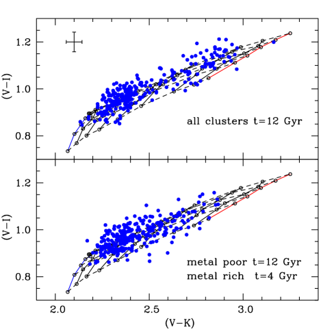
Figure 1: Integrated colours of clusters belonging to one single realization of the synthetic template population discussed in the text (upper panel). The 1$\sigma$ colour error bars are shown in the upper left corner of the panel. Also displayed is the reference grid of analytical integrated colours for selected metallicities and ages. Solid lines are constant [Fe/H] lines, dashed lines are constant age lines. Moving towards increasing $(V-I)$ colours, the reference ages are equal to 2, 4, 6, 9, 12 and 15 Gyr. Moving towards increasing $(V-K)$ colours, the [Fe/H] values are equal to $-$2.62, $-$2.14, $-$1.62, $-$1.31, $-$1.01, $-$0.70, $-$0.29, $-$0.09, 0.05. The lower panel displays one single realization of the bimodal-age population A discussed in the text.

Coming back to Fig. 1, an obvious point is to notice the important effect of the photometric error, even with a 1$\sigma$ error as small as 0.03 mag. Some objects appear younger than 2 Gyr when dated according to their location in the diagram, and many clusters appear older than 15 Gyr. Also the individual metallicities retrieved are obviously affected by the photometric errors, but the effect on the age is the most striking. This shows clearly that age-dating only a handful of objects in an extragalactic GC population can lead to erroneous results about the age distribution of the cluster system. Even when larger samples are observed, it is paramount that their colour-colour distribution is not biased compared to the case for the whole system.

As a second reference sample used in the comparisons that follow in the next section, we have created a synthetic GC system with an intrinsic bimodal-age population (labelled ’population A’). This system has the same properties of the template sample, the only difference being that the metal rich component is 4 Gyr instead of 12 Gyr old. The integrated colour-colour diagram of one realization of this bimodal-age population is displayed in the lower panel of Fig. 1; the analytical colour grid used to create this sample A is obviously the same employed for the template population, and it is also plotted in the diagram. To assess quantitatively the differences in the age distributions retrieved from the colour-colour diagram, we employ the cumulative age distributions – introduced by, e.g., Hempel et al. (hem03 (2003), hem04 (2004)) to establish statistically the existence of young subpopulations – as obtained from the individual cluster colours and the reference grid displayed in Fig. 1. The cumulative age distribution (CAD – number fraction of clusters with age larger than $t_{i}$ as a function of $t_{i}$) for one single realization of a synthetic cluster populations has been computed as follows. We associate to each cluster an age greater than $t_{i}$ when it lies above the line of constant $t_{i}$ (we considered $t_{i}$ values equal to 0, 2, 4, 6, 9, 12 and 15 Gyr) in the $(V-I)-(V-K)$ diagram. Objects below the 2 Gyr line are assigned to the bin corresponding to $t>t_{i}$=0 Gyr. Given the $(V-K)$ of an individual synthetic GC, we determine by linear interpolation within the reference grid the expected $(V-I)$ of the two neighbouring constant age lines at the cluster $(V-K)$. After this, it is straightforward to use the cluster $(V-I)$ to assign the object to the appropriate CAD age intervals. For the very few synthetic clusters – number of the order of unity – that appear in some realization beyond the red and blue $(V-K)$ edges of the theoretical calibration, we extrapolate the constant age reference colours by fitting the last three points of a given $t_{i}$ sequence with a function of the form $(V-I)_{t_{i}}=a+b\ {\rm ln}[(V-K)]$. The individual CAD number counts are then normalized to the total number of objects in each realization. In the Appendix we provide accurate fitting formulae $(V-I)_{t_{i}}=f[(V-K)]$ that can be applied to the whole $(V-K)$ range spanned by our theoretical colours, and allow a fast but still reliable estimate of the age distribution from the measured $(V-K)$ colours, without the need to interpolate within the reference colour grid.

Figures 2 and 3 show the CADs obtained from 30 realizations of, respectively, the template and the bimodal-age samples discussed above. Filled circles represent the mean of the results obtained from the multiple realizations, error bars show the 1$\sigma$ dispersion around these mean values. The size of the error bars associated to the individual points of the CAD is affected – keeping everything else unchanged – by the GC sample size, and increases when the number of synthetic GCs decreases (see also Hempel & Kissler-Patig hem04 (2004)).

Figure 2: CADs for the 12 Gyr template sample. The solid line displays the real age distribution, dotted and dashed lines the CAD retrieved from the colour-colour diagram for the full sample (dashed line) and for only the clusters with $(V-K)>$2.4 (dotted line – see text for details).

Figure 3: As in Fig. 2 but for population A with the bimodal age distribution. The upper panel shows the CADs for the whole sample (real age distribution – solid line; retrieved age distribution – dashed line) whereas the lower panel shows the age distribution only for clusters with $(V-K)>$2.4 (real age distribution – solid line; retrieved age distribution – dashed line).

Figure 2 shows very clearly the large change in the age distribution retrieved from the colour-colour diagram, compared to the input one (solid line). The ages retrieved for the whole sample (dashed line) span a range between 2 Gyr (or less) up to more than 15 Gyr, and the shape of the CAD is greatly changed, displaying a smooth decrease with $t_{i}$, because the synthetic clusters tend to be more evenly distributed over the reference clour grid. If we restrict the sample to the more metal rich objects, with $(V-K)>2.4$ (about half of the total sample falls into this colour interval, that corresponds to retrieved [Fe/H] values larger than $\sim-$ 1.0 to $-$1.3, using the calibration provided by the reference grid) the CAD is very similar, although not exactly identical. This is due to the different sensitivity of the colours to age (and also to metallicity) at different locations on the diagram. The case for the bimodal age distribution is displayed in Fig. 3. Again, the retrieved ages show a CAD very different from the real one; the trend with $t_{i}$ is, as expected, much smoother. Restricting the analysis the sample to objects redder than $(V-K)>2.4$ allows one to study a sample with a higher ratio of old to young objects, because we are mainly sampling the higher metallicity and younger clusters in the synthetic populations.

Figure 4: Comparison between the retrieved CADs for the 12 Gyr template (solid line) and the bimodal-age population A (dashed line). The upper panel displays the comparison for the full synthetic samples, the lower panel the comparison only for objects with $(V-K)>$2.4.

Figure 4 displays a comparison between the retrieved CADs of the two populations, for the full samples (upper panel) and for objects with $(V-K)>$2.4 only (lower panel). The difference between the two CADs is evident, in both the full and restricted samples. Bimodal-age CADs are always below the unimodal ones. This is the basis for the use of CDAs as indicators of age bimodality, as discussed in detail by Hempel & Kissler-Patig (hem04 (2004)). The sample with $(V-K)>$2.4 shows a larger difference between the two CADs, because in this colour range the ratio young/old clusters in the bimodal-age population is about 50%, whereas when the full sample is considered, it is only 25%.

The comparison presented in Fig. 4 summarizes the main results of this discussion about the CAD of our two reference synthetic populations. Bimodal-age (young+old) populations display a CAD systematically lower than the case of unimodal (old) populations. The extent of this difference depends on both the age of the young subpopulation and the number ratio between the two components. Increasing the ratio of young to old clusters – keeping the age distribution fixed – shifts the CAD towards increasingly lower values. The same happens when one decreases the age of the young component – keeping constant the number ratio between the two subpopulations – as we will show explicitely during one of the tests of the next section (analogous conclusions can be found in Hempel & Kissler-Patig hem04 (2004)).

Figures 5 and  6 display the cumulative [Fe/H] distribution (CMeD) from the same multiple realizations of the template and the bimodal-age A sample. As in case of the CAD, filled circles represent the mean of the results obtained from the various realizations, and error bars show the 1$\sigma$ dispersion around these mean values. For each realization we associate to an individual cluster an ${\rm[Fe/H]}>{\rm[Fe/H]}_{i}$ when it lies to the right of the line of constant ${\rm[Fe/H]}_{i}$ predicted by the reference grid. We considered ${\rm[Fe/H]}_{i}$ values equal to $-$2.62, $-$2.14, $-$1.62, $-$1.31, $-$1.01, $-$0.70, $-$0.29, $-$0.09, 0.05, as in Fig. 1. As for objects blueward of the [Fe/H]=$-$2.62 line – number usually of the order of unity – they are included into an additional bin corresponding to [Fe/H]$>{\rm[Fe/H]}_{i}=-4.5$, that is an arbitrary low value. The individual number counts of each CMeD are then normalized to the total number of objects in each realization. Similar to the case of the CAD, we determine the appropriate [Fe/H] bin of the individual objects by linear interpolation among the reference colour grid. For synthetic objects above the highest age of the reference grid, we extrapolate the constant [Fe/H] lines by approximating $(V-K)$ as a linear function of $(V-I)$, fitted to the last three points below the grid boundary, for each reference metallicity. For objects located below the 2 Gyr line we supplement the grid shown in Fig. 1 with the integrated colours of a 1 Gyr old population. If necessary, slightly younger ages are accounted for.

Figure 5: CMeDs for the 12 Gyr template sample. The solid line displays the real [Fe/H] distribution, dashed lines the CMeD retrieved from the colour-colour diagram for the full sample and for only the clusters with $(V-K)>$2.4. Here, as in all following figures displaying CMeDs, we do not show the bin corresponding to ${\rm[Fe/H]}_{i}>-4.5$, that always has a normalized number count equal to 1.

Figure 6: As in Fig. 5 but for population A with a bimodal age distribution. For comparisons we also display – dashed-dotted line – the corresponding CMeDs retrieved in the case of the 12 Gyr template.

The CMeDs plotted in Figs. 5 and  6 demonstrate how the input and retrieved CMeDs show only marginal differences. In the case of both the full sample and the $(V-K)>$ 2.4 one, input and retrieved metallicity distributions are very similar for both age distributions. The largest difference is at ${\rm[Fe/H]}_{i}=-$1.31 for the full samples, where the retrieved CMeDs show counts larger then the intrinsic one. This is due to the fact that the intrinsic [Fe/H] distribution shows a dip between the peaks associated to the two metallicity components, that falls into this [Fe/H] bin; the retrieved [Fe/H] values have however a much less pronounced dip due to the smoothing effect of the photometric error. An important result is that the different age distribution has only a small effect on the derived CMeD. This is clearly illustrated by Fig. 6, where the CMeDs retrieved from the template sample are also displayed.

4 Analysis of systematic effects

In this section we analyze to what extent systematic effects related to the unknown morphology of the horizontal branch in unresolved GCs, their unknown metal distribution, colour statistical fluctuations and the uncertain efficiency of convective core overshooting, are able to change the CAD retrieved using a fixed reference grid of analytical integrated colours. As already mentioned in the introduction, our main goal is to establish whether these effects are able to mimic a bimodal-age distribution in presence of an uniformly old stellar population. We also wish to assess the possible occurrence of biases in the cluster metallicity distribution inferred from the colour-colour diagram, as compared to the intrinsic one.

The general method of analysis is the following. We create synthetic populations with the same $t$, [Fe/H], $M_{t}$, photometric error distributions of a reference system – this latter determined using our reference colour grid displayed in Fig. 1; a reference system could be our template single-age or the bimodal-age population A described in the previous section – but using integrated magnitudes that include the effect of, for example, a different HB morphology. Table 1 summarizes the main properties of all the synthetic GC samples employed in these tests.

We then retrieve the age and [Fe/H] distributions of these new synthetic samples by employing our reference grid (that does not take into account, e.g., the different HB morphology) and compare the results with those obtained for the reference systems.

Table 1: Main properties of the synthetic GC samples discussed in this paper (see text for details).

Label	Mass + [Fe/H]	Age	Mass loss	Convection	Metal mixture	1$\sigma$ phot. error	Colour computation
Template	Milky Way GCs	12 Gyr	$\eta$=0.2	No-oversh.	$\alpha$-enh.	0.03 mag	Analytic
A	Milky Way GCs	12+4 Gyr	$\eta$=0.2	No-oversh.	$\alpha$-enh.	0.03 mag	Analytic
B	Milky Way GCs	12 Gyr	$\eta$=0.4	No-oversh.	$\alpha$-enh.	0.03 mag	Analytic
B2	Milky Way GCs	12 Gyr	bimodal $\eta$=0.2,0.4	No-oversh.	$\alpha$-enh.	0.03 mag	Analytic
C	Milky Way GCs	12 Gyr	$0.2\leq\eta\leq$ 0.4	No-oversh.	$\alpha$-enh.	0.03 mag	Analytic
D	Milky Way GCs	12 Gyr	$\eta$=0.2	No-oversh.	$\alpha$-enh. + scaled solar	0.03 mag	Analytic
E	Milky Way GCs	12 Gyr	$\eta$=0.2	No-oversh.	$\alpha$-enh.	0.03 mag	Monte-Carlo
F	Milky Way GCs	12+4 Gyr	$\eta$=0.2	No-oversh.	$\alpha$-enh.	0.03 mag	Monte-Carlo
G	Milky Way GCs	12+2 Gyr	$\eta$=0.2	No-oversh.	$\alpha$-enh.	0.03 mag	Analytic
H	Milky Way GCs	12+2 Gyr	$\eta$=0.2	Oversh.	$\alpha$-enh.	0.03 mag	Analytic
I	Milky Way GCs	12 Gyr	$\eta$=0.2	No-oversh.	$\alpha$-enh.	0.10 mag	Analytic
J	Milky Way GCs	12 Gyr	$\eta$=0.4	No-oversh.	$\alpha$-enh.	0.10 mag	Analytic

The quantitative results of these comparisons are inevitably dependent on the assumed photometric error, [Fe/H], age and – in some case – $M_{t}$ distribution of the synthetic GCs. With the exception of the photometric error, that when largely increased tends to wash out all other effects, the general trends should be unaffected by the precise choices made about these parameters, and provide useful guidelines to understand the impact of these uncertainties on our interpretation of extragalactic GC systems. We employed throughout our analysis the [Fe/H], $t$ and $M_{t}$ distributions of a real GC system, e.g. the Galactic one, already introduced in the previous section. As for the photometric error, we continue to use a 1$\sigma$=0.03 mag value, that corresponds to accurate photometry of Galactic GCs. The size of our synthetic samples are also large – the same as the template and the bimodal-age ones introduced in the previous section. This combination of – realistic – ’small’ photometric error and large sample size, highlights more clearly the role played by the uncertainties we are going to address. As mentioned previously, the effect of reducing the sample size is purely to increase the error bars attached to the individual points of the retrieved CADs and CMeDs. The effect of increasing photometric errors will be addressed at the end of this section.

4.1 Horizontal Branch morphology

To date, the theory of stellar evolution is unable to predict from first principles the expected morphology of the HB in an old stellar population of fixed age and chemical composition. This arises from the lack of a theory for the stellar mass loss along the RGB phase. Once age and chemical composition are fixed, the HB morphology is completely determined by the amount of mass lost along the RGB phase by the progenitor objects. From synthetic HB modelling we know that stars along the RGB phase have to lose on average $\sim$0.10–0.20$M_{\odot}$ in order to reproduce the typical colour location of the HBs observed in Galactic GCs, and a 1$\sigma$ spread of the order of $\approx$0.02$M_{\odot}$ around this mean mass loss value has to be typically considered to match the observed HB colour extension (see, e.g., Lee, Demarque & Zinn ldz94 (1994)). However, the precise values may differ from cluster to cluster and are in principle unknown for extragalactic unresolved GCs.

Observational determinations of mass loss rates along the RGB are scarce (see, e.g. Origlia et al. of02 (2002)) and have not led yet to a mass loss theory with predicting power. The Reimers (rei75 (1975)) mass loss formula is traditionally used in stellar evolution modelling; it contains a free parameter $\eta$, whose value determines the efficiency of the mass loss process (see also Catelan cat06 (2006) for a summary of alternative, but less used mass loss formulae).

Figure 7: Comparison of the HB evolution in the magnitude-effective temperature plane, for 12 Gyr old isochrones computed with the mass loss parameter $\eta$=0.2 (solid line) and 0.4 (dashed line) respectively, and the two labelled metallicities. The $V$, $I$ and $K$ labels denote the photometric filter used for each of the three pairs of tracks represented in each of the two panels.

A quantitative example of the effect of different RGB mass loss assumptions on the HB magnitudes and colours is shown by Figure 7. Here we display the magnitude-$T_{eff}$ HB sequence for a 12 Gyr $\alpha$-enhanced isochrone and the two labelled [Fe/H] values (that correspond approximately to the mean values for the two metallicity components of our synthetic GC populations) for $\eta=0.2$ (the value adopted in our template GC sample) and 0.4. These two values of $\eta$ produce a total RGB mass loss equal to, respectively, 0.08$M_{\odot}$ and 0.17$M_{\odot}$ at [Fe/H]=$-$1.6; 0.10$M_{\odot}$ and 0.20$M_{\odot}$ at [Fe/H]=$-$0.7. Larger mass loss implies a hotter HB, due to the smaller ratio between total mass and He-core mass; this can be clearly seen in the figure, together with the fact that the effect is much larger at the lower metallicity. The magnitude of the Zero Age HB (ZAHB) location (stars spend most of their HB evolution near the ZAHB location) becomes fainter by a large amount in $I$ (about 0.8 mag) and even more in $K$ (about 1.5 mag) when $\eta$ is doubled and [Fe/H]=$-$1.6. As a general rule and for all metallicities, the size of the magnitude change depends on the photometric filter one considers.

Uncertain predictions of the HB morphology in unresolved GCs lead to uncertainties in the predicted integrated magnitudes and colours, given that the HB phase is bright and relatively long-lived, and accounts for a non-negligible fraction of the cluster integrated flux.

Figure 8: Comparison between the retrieved CADs for the 12 Gyr template (solid line) the $\eta=0.4$ population B (dashed-dotted lines) and the bimodal $\eta$ population B2 (dotted line). The upper panel displays the comparison for the full synthetic samples, the lower panel the comparison only for objects with $(V-K)>$2.4 (the results for population B2 are not displayed in this panel, because they are identical to the case of the template population). The corresponding CADs for the bimodal-age population are also displayed as dashed lines.

To give a quantitative estimate of how a wrong assumption about the unknown HB colour affects the ages derived from the $(V-K)-(V-I)$ plane, we first created a synthetic GC population labelled ’population B’) with exactly the same properties of the 12 Gyr template one, but employing isochrones computed with $\eta$=0.4, i.e., with a bluer HB. We then determined the CAD for 30 realizations of this sample, using the reference grid of our template population (with $\eta$=0.2). The resulting CAD is displayed in Fig. 8, compared to the results for the template population and the bimodal-age population A discussed in the previous section.

When the whole cluster samples are compared, population B shows an age distribution very similar to the bimodal-age population A, whereas if we consider only objects with $(V-K)>$2.4, there is essentially no difference compared to the result for the template population. This is because at [Fe/H]$<-$1.6 the bluer HB morphology affects strongly the integrated colours, that become bluer and mimic a much younger age if the CAD is determined from the reference ($\eta$=0.2) colour grid. This effect is negligible at higher metallicities because the HB colour and magnitude change only slightly when doubling $\eta$ (see Fig. 7). Of course, if the mass loss is so high as to produce a much bluer HB also at [Fe/H]$>-$1.0, then we would retrieve substantially young ages also for the cluster with $(V-K)>$2.4.

Figure 9: As in Fig. 8, but for the comparison with the 12 Gyr old, extended HB population C (dashed-dotted line).

As a second experiment, we tested the influence of having clusters with the same [Fe/H] but different mass loss efficiencies along the RGB. This effectively means that GCs with the same metallicity (and age) can have different HB morphologies (as actually observed in the Galaxy, like in case of the cluster pair M3-M13). To this purpose we created a 12 Gyr GC population (labelled ’population B2’) with the same properties of the template sample, but where 50% of the synthetic clusters with [Fe/H]$<-$1.1 (we saw before that changing $\eta$ from 0.2 to 0.4 does not have an appreciable effect on the retrieved CAD at higher metallicities) is originated from isochrones computed with $\eta$=0.4, and the remaining 50% from isochrones with with $\eta$=0.2 (bimodal $\eta$ distribution). The retrieved CAD is displayed in the upper panel of Fig. 8 for 30 realizations of this sample, using the reference grid of our template population (with $\eta$=0.2). The CAD lies, as expected, above the case of population B ($\eta$=0.4 for all clusters) but it is still very close to the bimodal-age population A for ages above 9 Gyr. Of course, a reduced fraction of clusters with $\eta$=0.4 would move the CAD towards the template case.

As a third quantitative test, we have determined a synthetic population with an HB extended in colour (labelled ’population C’) more similar to the HBs observed in real GCs. The mass distribution along the HB is assumed to have a flat profile between the values corresponding to $\eta$=0.2 and 0.4. Figure 9 compares the retrieved CADs with the template and the bimodal-age population A. Predictably, the effect on the whole sample is smaller, and the CADs is halfway between the template and population A. Clusters with $(V-K)>$2.4 are unaffected. A very similar CAD, slightly closer to the template case, is found from a synthetic GC sample identical to population C, but with an HB morphology obtained employing a mean HB mass obtained from a $\eta$=0.3 mass loss parameter along the RGB, and a 1$\sigma$ dispersion of 0.015$M_{\odot}$ around this mean value . This type of mass distribution produces a relationship between [Fe/H] and the HB morphology parameter $HB_{t}=(B-R)/(B+V+R)$ (where $B$, $V$ and $R$ are in this case the number of HB stars bluer than the RR Lyrae instability strip, within the strip, and redder than the strip, respectively. We employed the relationships by Di Criscienzo, Marconi & Caputo dic04 (2004) for identifying the position of the RR Lyrae instability strip in our simulations) close to the mean relationship for Galactic GCs, as obtained from data in the Harris (har96 (1996)) catalogue.

The main conclusion of all these tests is that the unknown morphology of the HB in an unresolved GC population has the potential to strongly affect the cluster CADs – particularly at low-intermediate metallicities – and mimic an old+young bimodal-age population, even in the case where all clusters are old.

Figure 10: As in Fig. 5 but for the comparison with the 12 Gyr old population B with $\eta$=0.4 mass loss law (see text for details).

Figure 11: As in Fig. 5 but for the 12 Gyr old population C with the extended HB (see text for details).

The retrieved CMeDs for the two blue-HB synthetic populations B and C are displayed in Figs. 10 and 11, compared to the intrinsic ones. Differences with respect to the intrinsic CMeDs are generally small. At lower [Fe/H] below $\sim-$0.7 the retrieved CMeDs display systematically (slightly) lower number fractions compared to the intrinsic values, and it is due to the effect of a larger mass loss, that affects mainly the low-intermediate metallicities, and causes bluer integrated colours. This affects not only the age estimate, but also the retrieved [Fe/H] values. The CMeD for the sample B2 is intermediate between the results for populations B and C.

4.2 Scaled solar vs $\alpha$-enhanced mixtures

The initial metal distribution of extragalactic GCs for which we are able to measure only integrated colours is in principle unknown. One can use as a guideline the fact that the Galactic GC system displays an $\alpha$-enhanced metal mixture (see, e.g., Carney c96 (1996)) but this might not be the case in other GC systems.

Figure 12: Lines of constant age in the $(V-K)-(V-I)$ diagram for scaled solar (solid lines) and $\alpha$-enhanced (dashed lines) metal mixtures, as obtained from the analytical relationships given in the Appendix. Ages are the same as in Fig. 1 and increase from bottom to top.

We display in Fig. 12 lines of constant age in the $(V-K)-(V-I)$ diagram, for both scaled solar and $\alpha$-enhanced metal mixtures, in the $(V-K)$ range spanned by the $\alpha$-enhanced calibration. For ease of interpretation, the smooth constant-age lines have been determined using the analytical relationships given in the Appendix. The scaled solar colours have also been obtained from models in the BaSTI database and are homogeneous with the $\alpha$-enhanced ones. The differences in the two theoretical calibrations are evident. At the bluest end (i.e. at the lowest [Fe/H]) of the theoretical calibration the colour differences are small, but they increase sharply with increasing $(V-K)$, e.g, [Fe/H]. The net effect is to assign too young ages to GCs with scaled solar metal mixtures when an $\alpha$-enhanced calibration is used. Of course the reverse is true when determining ages of $\alpha$-enhanced GCs with a scaled solar calibration.

Figure 13: Comparison between the retrieved CADs for the 12 Gyr template (solid line) and population D (dashed-dotted lines) whose metal rich subpopulation is assumed to be born out of a scaled solar metal distribution. The upper panel displays the comparison for the full synthetic samples, the lower panel the comparison only for objects with $(V-K)>$2.4. The corresponding CADs for the bimodal-age population A are also displayed as dashed lines.

To give more quantitative estimates of this effect we have created a synthetic sample (labelled ’population D’) with the same properties as the 12 Gyr template one, but employing a scaled solar metal mixture for the metal rich component, i.e. the component centred around [Fe/H]=$-$0.55. We then retrieved the CADs and CMeDs of this system with our reference $\alpha$-enhanced colour grid. Figure 13 compares the CADs for this whole new sample and the $(V-K)>$2.4 clusters only, with the corresponding template and bimodal-age population A ones. The “erroneous” metal mixture attributed to the metal rich component simulates a bimodal-age population, albeit with a smaller age difference than our 12+4 Gyr system. The effect is clearly enhanced when the sample is restricted to only the more metal rich clusters with $(V-K)>$2.4.

Figure 14: As in Fig. 5 but for the 12 Gyr old Population D with a scaled solar metal rich subpopulation.

The corresponding CMeDs are compared in Figure 14. The differences with respect to the intrinsic distributions are small, almost identical to the case of the template and bimodal-age samples shown in Figs. 5 and 6. This means that the metal mixture does not influence appreciably the retrieved [Fe/H] distributions, at least for the two specific mixtures used in this test.

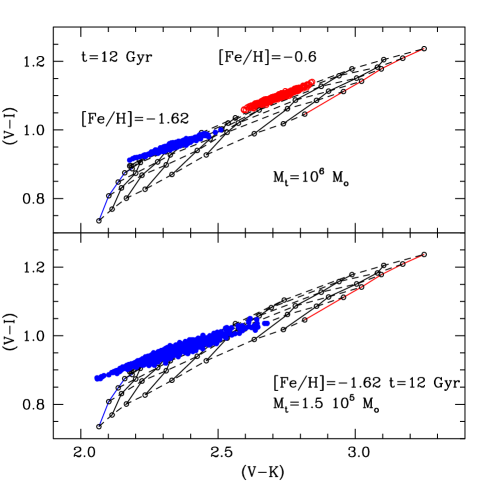
Figure 15: Monte-Carlo integrated colours of 500 realizations of a 12 Gyr old GC populations with the labeled total masses and [Fe/H] (see text for details).

4.3 Statistical fluctuations

In Section 2 we already discussed the fact that when the number of objects harboured by a stellar system is not large enough to sample smoothly all evolutionary phases, statistical fluctuations of its integrated colours do arise, caused by stochastic variations of the number of objects populating the faster evolutionary phases.

The effect on the $(V-I)-(V-K)$ plane is shown by Fig. 15, where we display the integrated colours obtained from 500 realizations of a 12 Gyr old population with [Fe/H]=$-$1.62, and two different values of the total mass $M_{t}$, namely $M_{t}=1.5\ 10^{5}M_{\odot}$ (that is the value corresponding to the peak of the GCLF) and $M_{t}=10^{6}M_{\odot}$. For each realization we have determined the integrated colours using the Monte-Carlo procedure presented in Section 2.

The points are centred around the corresponding analytical values of the integrated colours, with a large scatter. The total $(V-K)$ range is of the order of $\approx$0.6 mag for $M_{t}=1.5\ 10^{5}M_{\odot}$, and $\approx$0.4 mag for $M_{t}=10^{6}M_{\odot}$. The total $(V-I)$ range is $\approx$0.2 mag for $M_{t}=1.5\ 10^{5}M_{\odot}$ and $\approx$0.1 mag for $M_{t}=10^{6}M_{\odot}$. There is a clear correlation between the fluctuations of the two colours. The scatter decreases with increasing cluster mass, due to a better sampling of the faster evolutionary phases when the cluster mass (hence the total number of stars) increases. The $(V-K)$ colour fluctuates more than $(V-I)$, because the integrated flux in the $K$-band is more affected than the $I$-band by the AGB and bright RGB evolutionary stages, that are the fastest ones and more prone to statistical number fluctuations. Due to these fluctuations only (we did not include any photometric error in the simulations displayed in Fig. 15) the [Fe/H] value retrieved for an individual cluster can be wrong by as much as $\approx$1 dex in the low metallicity regime. Retrieved ages can also be biased by several Gyr.

Figure 15 shows also the colour fluctuations associated to a 12 Gyr GC with [Fe/H]=$-$0.6. It is important to notice that in this case the distribution of points is almost parallel to the constant age line. This means that at the upper end of the Galactic GC metallicity distribution, statistical colour fluctuations have a minor effect on the age estimates using the $(V-K)-(V-I)$ diagram.

To study the effect of colour fluctuations on the retrieved age distribution of an entire GC system, instead of a single cluster – including the presence of 0.03 mag 1$\sigma$ photometric errors – we have determined one synthetic population corresponding to the template one, and one corresponding to the bimodal-age (12+4 Gyr) population, but this time the integrated colours of the individual clusters are determined following the Monte-Carlo procedure explained in Section 2 (these two populations are labelled ’population E’ and ’F’, respectively). The analysis of these two samples allows us to check, among others, whether statistical fluctuations can in principle erase the difference between single-age and bimodal-age CADs. We stress that the inclusion of statistical fluctuations is in principle necessary to realistically reproduce the integrated photometry of observed GCs, unless they have a mass distribution shifted towards masses much larger than the Galactic counterpart.

In Figs. 16 and 17 we have compared the CADs retrieved for these two populations E and F, with those obtained for exactly same GC properties but with integrated colours computed analytically.

Figure 16: Comparison between the retrieved CADs for the 12 Gyr template (solid line) and population E, that accounts for statistical fluctuations of the star number counts (dashed-dotted lines). The upper panel displays the comparison for the full synthetic samples, the lower panel the comparison only for objects with $(V-K)>$2.4. The corresponding CADs for the bimodal-age population A with analytical integrated colours are also displayed as dashed lines.

The general trends are clear. When only objects with $(V-K)>$2.4 are considered, the CADs are essentially unchanged compared to the case of analytical colours. This is a consequence of the fact that at high metallicities the colour fluctuations do not significantly affect the individual age estimates (see Fig. 15). Very different is the case when the whole samples are considered. The inclusion of the more metal poor clusters causes a significant change of the CAD, compared to the case of analytical colours. Significant differences start between the 6 Gyr and the 9 Gyr age bin. The CAD that accounts for the statistical fluctuations is above the CAD for the analytical case, with a larger percentage of objects at high ages. This behaviour is very similar for both the single-age (Fig. 16) and bimodal-age (Fig. 17) populations

Figure 17: Comparison between the retrieved CADs for the 12 Gyr template (solid line) and the bimodal age population F, with integrated colours computed via a Monte-Carlo simulation (dashed-dotted lines). The upper panel displays the comparison for the full synthetic samples, the lower panel the comparison only for objects with $(V-K)>$2.4. The corresponding CADs for the bimodal-age population A with computed analytical colours are also displayed, as dashed lines.

To summarize, the effect of statistical colour fluctuations on the retrieved CADs is negligible if only the redder clusters are analyzed. When the full GC samples are considered, a proper inclusion of statistical colour fluctuations tend to shift the retrieved CADs towards higher values – for ages $t_{i}>$6 Gyr – compared to the case when they are neglected. This behaviour is very similar for both the single-age (Fig. 16) and bimodal-age (Fig. 17) populations. As a consequence, relative differences between single-age and bimodal-age CADs are preserved.

As for the [Fe/H] distribution, the retrieved CMeDs that include the effect of colour fluctuations are displayed in Figs. 18 and 19, compared to the intrinsic CMeDs. First, one can immediately notice that, again, the assumed age distribution does not play a significant role in the outcome of this comparison. In general, the number fractions for the full samples (with the exception of the point at [Fe/H]=$-$4.5, that by definition is always equal to unity for both intrinsic and retrieved CMeDs) are typically lower than the intrinsic CMeDs when [Fe/H] is below $\sim-$1.6. This is due to a sizable fraction of metal poor objects with anomalously blue $(V-K)$ colours, that are assigned a [Fe/H]$<-$2.62. At higher metallicities the differences with respect to the intrinsic CMeDs tend to be smaller, and only slightly larger than in case of photometric errors only (see Figs. 5 and 6).

Figure 18: As in Fig. 5 but for the 12 Gyr old population E that accounts for colour statistical fluctuations.

As an interesting detail, one can notice that the intrinsic [Fe/H] (solid lines in Figs. 18 and 19) of objects with $(V-K)>$2.4 can reach values even lower than [Fe/H]=$-$1.62. In fact, the intrinsic CMeD corresponding to ${\rm[Fe/H]}_{i}>-$1.62 displays a value below unity; if all clusters in the sample have an intrinsic [Fe/H] higher than this value, the corresponding CMeD would show a value equal to unity at this point. Why do we find such metal poor clusters in the red subsample? This occurrence is not mainly due to the photometric error employed in the simulation – Figures 5 and 6 display values approximately equal to unity at this [Fe/H] – rather to the colour fluctuations of the most metal poor objects, that can appear at anomalously blue but also anomalously high $(V-K)$ colours (see Fig. 15). As a consequence the intrinsic CMeD of the $(V-K)>$2.4 subsamples will contain anomalously metal poor objects. Another consequence is that the retrieved metallicity of these anomalously red objects is much higher than their intrinsic one, when estimated from their position in the colour-colour plane. This explains why the retrieved CMeD at ${\rm[Fe/H]}_{i}=-$1.62 displays a value much closer to unity, compared to the intrinsic one.

Figure 19: As in Fig. 5 but for the bimodal-age population F that accounts for colour statistical fluctuations.

Before closing this discussion on colour fluctuations, we wish to address a further important point. Observations of distant GC systems usually can acquire sufficiently precise photometry of only the brightest clusters, populating the bright tail of the GCLF. Brightest clusters means the most massive ones, for which the effect of statistical colour fluctuations is smaller. To simulate this effect and check the consequences on CAD and CMeD, we selected from our populations E and F only objects with integrated $M_{V}<-$8.5 that corresponds to $M_{t}$ larger than $\sim 3\ 10^{5}\leavevmode\nobreak\ M_{\odot}$. The resulting samples contain about 60 objects, therefore the error bars on the individual points of the retrieved CADs and CMeDs will be larger than in the previous case.

Figure 20: Retrieved CADs for the 12 Gyr population E (upper panel) and the bimodal-age population F (lower panel), with integrated colours computed via a Monte-Carlo technique. Dashed-dotted lines represent the case of GC subsamples with integrated $M_{V}<-$8.5 (about 60 clusters for each Monte-Carlo realization). Solid lines display the CADs retrieved for the full samples corresponding to the template and population A, with integrated colours computed analytically (see text for details).

Figure 20 compares the retrieved CADs of the single-age population E and bimodal-age population F (that include colour fluctuations) restricted to $M_{V}<-$8.5, with the results for the full template and population A. The effect of statistical fluctuations on the ages is now almost negligible.

The retrieved CMeD of the population E sample ( restricted to $M_{V}<-$8.5) is compared to the intrinsic one in Fig. 21 (analogous result is obtained for the bimodal-age sample) and shows at low [Fe/H] much smaller differences compared to the intrinsic CMeD than the case displayed in Fig. 18, because of the reduced fluctuations.

As a general conclusion of this further test, colour fluctuations do not play a relevant role in the determination of the age and [Fe/H] distributions from the integrated $(V-I)-(V-K)$ diagram, when one restricts the analysis to GCs brighter than $M_{V}=-$8.5.

Figure 21: As in the upper panel of Fig. 19 but for the sample restricted to objects with $M_{V}<-$8.5 (see text for details).

4.4 Core overshooting

There is an ongoing debate about the possibility that in stars with convective cores along the Main Sequence (i.e., with mass larger than $\sim$ 1.1- 1.2$M_{\odot}$) the motion of the convective fluid elements is not halted shortly beyond the boundary with the stable radiative region as determined by the Schwarzschild criterion, but it goes on for an appreciable length within the formally stable surrounding layers (overshooting). The extent of the overshooting region is the focus of many investigations like, among the most recent ones, those by Testa et al. (tfc99 (1999)), Woo & Demarque (wd01 (2001)) and Barmina, Girardi & Chiosi (bgc02 (2002)). The presence of efficient overshooting from Main Sequence convective cores alters both colour and luminosity of the isochrones Turn Off (such that the Turn Off is generally brighter and hotter at fixed age) thus affecting integrated colours of an SSP of fixed age and chemical composition.

This issue is irrelevant for Galactic globular clusters, given that they harbour stars with mass low enough not to experience the onset of convective cores along the Main Sequence phase; however, in presence of bimodal-age populations with a component only a few Gyr old, this phenomenon can play a role.

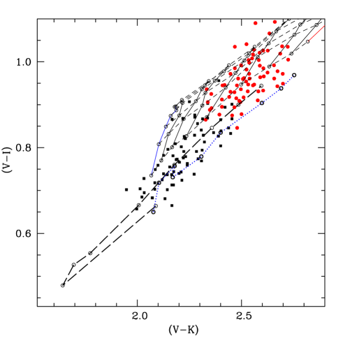
Figure 22: Colour-colour diagram of two 2 Gyr old synthetic GC populations (80 clusters each) with [Fe/H]=$-0.55\pm 0.20$, computed using models with (black filled squares) and without (red filled circles) core overshooting. The reference colour grid of Fig. 1 is also displayed, together with the 2 Gyr constant age line obtained from models that include overshooting (thick dashed line) and the 1 Gyr constant age sequence from models without overshooting (dotted line – see text for details). The [Fe/H] values decrease moving away from the point with the largest $(V-K)$ value, along the constant age line.

Figure 22 displays our reference $\alpha$-enhanced colour grid shown in Fig. 1, obtained from models without overshooting, with the addition of the 1 Gyr old sequence. Colours predicted by $\alpha$-enhanced models including overshooting (calculated from isochrones in the BaSTI database, that employ the overshooting treatment discussed by Pietrinferni et al. pietr04 (2004)) are the same as the reference grid, when the age is equal or larger than 4 Gyr. At younger ages convective overshooting starts to play a role. For the sake of comparison we display in Fig. 1 also the 2 Gyr constant age line obtained from models including overshooting.

Quantitative and qualitative differences between the 2 Gyr lines with and without overshooting are remarkable. On the whole the 2 Gyr overshooting colour-colour sequence lies between the 1 Gyr and 2 Gyr non overshooting ones. More specifically, for a given age and [Fe/H] pair, the $(V-I)$ and $(V-K)$ colours of the 2 Gyr overshooting models are systematically bluer than the values of the reference grid at 2 Gyr; the trend of both colours with [Fe/H] at constant age is non-monotonic in the overshooting case, because of the turn to the red (in both $(V-K)$ and $(V-I)$) occurring between the two lowest metallicity points. The 1 Gyr non-overshooting line shows also signs of a non-monotonic behaviour at low metallicities. These are due to the complex interplay between the variation of Turn Off colours, colour extension of the blue loops during the central He-burning phase and brightness of the RGB phase with changing [Fe/H].

Figure 23: CADs retrieved using the reference non-overshooting color-colour calibration of Fig. 1 for the 12+2 Gyr bimodal-age populations H (dotted line) and G (dashed line). The CAD retrieved for the template (thick solid line) and the bimodal-age population A (thin solid line without symbols) are also displayed. The upper panel displays the CADs for the full samples, the lower panel the case of objects with $(V-K)>$2.4.

To highlight further the effect of convective overshooting on integrated colours, Fig. 22 shows also the colour-colour diagram of two synthetic samples (80 objects each) of 2 Gyr old clusters with [Fe/H]=$-0.55\pm 0.20$ (i.e. the [Fe/H] distribution of the metal rich components of all synthetic populations discussed in this paper) and 1$\sigma$ photometric errors of 0.03 mag, computed from $\alpha$-enhanced $\eta$=0.2 models both with and without convective overshooting during the Main Sequence phase. The inclusion of overshooting, as expected, makes the synthetic clusters bluer on average in both colours. This certainly affects the retrieved CADs and CMeDs, if an inconsistent colour-colour calibration is used.

For a quantitative assessment of this effect we have created a bimodal-age population with the same [Fe/H] distribution as the template sample, a 12 Gyr age for the metal poor component, and a 2 Gyr age for the metal rich one. Photometric errors are as in the template sample. We computed the integrated colours analytically using the $\eta$=0.2 $\alpha$-enhanced isochrones, both with (this population is labelled ’population H’) and without (this population is labelled ’population G’) overshooting for the case of the 2 Gyr clusters.

Figure 23 displays the CADs retrieved using the reference non-overshooting color grid for both populations G and H, compared to the results for the template sample, and for the bimodal (12+4 Gyr) population A.

Figure 24: CMeDs retrieved for populations G and H. Dashed lines and filled symbols correspond to population G, dotted lines and open symbols to population H. Solid lines with filled and open symbols are the input CMeDs for populations G and H, respectively. The top panel shows the comparison for the full samples, the bottom panel the case of objects with $(V-K)>$2.4.

We first discuss the comparison between the two 12+2 Gyr populations H and G, with and without overshooting. When the full samples are considered, the sample that includes overshooting displays a CAD differing from the non-overshooting one only in the youngest bins. This is easy to understand from Fig. 22; the “overshooting” 2 Gyr old population is located almost always below the 2 Gyr line of the reference colour grid, whereas the “non-overshooting” population of the same age is – obviously – more evenly distributed around the 2 Gyr line of the reference grid. This explains the appreciable difference between the two CADs in the bins corresponding to objects with ages larger than 2 and 4 Gyr, respectively. Differences decrease with increasing age because the contribution of the young population decreases sharply, and what dominates is the 12 Gyr old component which is unaffected by overshooting.

When we restrict the comparison to objects redder than $(V-K)$=2.4, the differences are more extreme. In this colour range there are very few 2 Gyr old clusters for population H (see again Fig. 22) so that the large majority of objects belong to the old metal poor 12 Gyr component. The CAD of population G shows predictably much lower number fractions, because of the presence of 2 Gyr old objects in addition to the 12 Gyr old component. Also, the number of clusters in this colour range is only about 25% of the total sample for the overshooting case, whereas the same fraction is about 50% for the non-overshooting sample. This smaller sample size explains the larger error bars attached to population H CAD when compared with population G.

We now compare the CAD of these two 12+2 Gyr populations with our 12 Gyr template sample and the bimodal population A with 12+4 Gyr old subpopulations. As expected, the CADs of both 12+2 Gyr systems have systematically lower values at each age bin than the CADs of both the template and population A. In case of objects redder than $(V-K)$=2.4 the CAD of population H population is now very close to the template one, because it contains essentially only 12 Gyr old objects. This means that an analysis restricted to this colour range would assign to this bimodal population an essentially constant and old age. On the other hand the CAD of the non overshooting population G shows, as expected, lower number fractions than the template and population A, even when the analysis is restricted to the redder clusters.

We can now summarize the effect of Main Sequence convective core overshooting on the retrieved CAD. When a colour grid that does not include core overshooting is used to retrieve ages of a young component where overshooting is efficient, the retrieved CAD is biased towards young ages in the age interval below $\sim$ 4 Gyr. If the analysis is restricted to the redder clusters, the retrieved CAD lacks almost completely the young component. An interesting consequence is that when one restricts the analysis to objects redder than a given $(V-K)$, there is the possibility to overlook the presence of a young component if the treatment of core convection in the models is not adequate.

Turning now to the estimate of the [Fe/H] distributions, the CMeDs retrieved for the two bimodal-age populations G and H are displayed in Fig. 24. The CMeD of population G shows only minor deviations from the input one, whereas in case of population H the most evident difference is the drop between ${\rm[Fe/H]}_{i}=-$1.31 and $-$1.01 when the full sample is considered. This is due to the systematically lower [Fe/H] estimated for the metal rich 2 Gyr component (see Fig. 22) whose retrieved [Fe/H] has in fact a sharp drop around [Fe/H]$\sim-$1. When the analysis is restricted to objects redder than $(V-K)$=2.4, population H is almost completely lacking the young metal rich component, located at bluer colours. Compared to the case of population G, both input and retrieved CMeDs display a large drop between ${\rm[Fe/H]}_{i}=-$1.62 and $-$1.01, because they are sampling essentially the high-metallicity tail of the metal poor old subpopulation.

4.5 Varying the 1$\sigma$ photometric error

For a given $M_{t}$, [Fe/H] and age distribution of the synthetic GC systems, the magnitude of the photometric error can affect the quantitative results of our comparisons (see the discussion in Hempel et al. hem04 (2004)). We briefly investigate here what happens if we consider photometric errors larger than our assumed value of 0.03 mag. We examine the cases of the template 12 Gyr sample, and the 12 Gyr $\eta=0.4$ opopulation B, discussed in Section 4.1. This latter sample is the one whose retrieved CAD appears to be the most discrepant from the template one (see upper panel of Fig. 8), approximately comparable to a bimodal 12+4 Gyr population A with $\eta$=0.2.

Figure 25 displays the CAD retrieved from a population (labelled ’population I’) analogous to the 12 Gyr template, but including a 1$\sigma$ photometric error equal to 0.10 mag. Compared to the template CAD of Fig. 2 one can notice a steeper slope at young ages and a flatter one at older ages. This reflects the much larger dispersion of points in the colour-colour diagram, with sizable numbers of clusters younger than 2 Gyr or older than 15 Gyr.

Figure 25: Comparison between the retrieved CADs for population I and J (see text and Table 1 for details) that include 1$\sigma$ photometric errors equal to 0.10 mag . The upper panel displays the comparison considering the full cluster samples, the lower panel the comparison restricted to clusters with $(V-K)>$2.4.

We have plotted in the same figure also the CADs retrieved by applying our reference grid to a population (labelled ’population J’) analogous to the 12 Gyr GC sample with $\eta$=0.4, but including again a 1$\sigma$ photometric error equal to 0.10 mag. Comparisons with population I show that the retrieved CADs are almost identical when considering both the whole populations or the redder clusters only.

This result shows that 1$\sigma=$0.10 mag photometric errors are sufficient to erase all the systematic effects (the conclusion for the CMeDs is similar) discussed in this paper. Given the similitude between the CADs retrieved for a 12 Gyr old GC sample with $\eta$=0.4 and the bimodal 12+4 Gyr population with $\eta$=0.2 (see Section 4.1) Fig. 25 implies also that bimodal age populations with age differences of up to 8 Gyr go undetected from CAD analyses, in presence of photometric errors of this magnitude.

5 Summary and discussion

In the previous section we have extensively studied the effect of inconsistent HB morphology, metal mixture and treatment of core convection between a synthetic sample of GCs (corresponding to an hypothetical observed system) and the reference colour grid used to retrieve their age and [Fe/H]. We also investigated the role played by statistical colour fluctuations due to the low $M_{t}$ of GCs. For all our tests we have created synthetic GC samples with $M_{t}$ (composite power law with two different slopes) and [Fe/H] (bimodal metal rich + metal poor components) distributions appropriate for the Galactic GC system, and a 1$\sigma$ photometric error typical of the integrated colours of Galactic globulars. The photometric error only is able to transform a constant or bimodal age distribution into an age distribution that covers smoothly a larger age range, as shown already by Hempel & Kissler-Patig (hem04 (2004)) . In addition to this smoothing, due purely to photometric errors, the results of our analysis can be summarized as follows:

• All effects studied in this paper may modify, to various degrees, the GC age distributions obtained from integrated $(V-K)-(V-I)$ diagrams. The retrieved [Fe/H] distributions are overall less affected.

• An HB morphology bluer than the one adopted for the reference colour grid used to estimate the GC ages can simulate a bimodal-age population (old + young components) even if all GCs are coeval. This is true both in case of a bluer morphology for the whole cluster sample, or when a substantial fraction of clusters has a bluer HB than accounted for in the theoretical colour grid. For the mass loss laws employed in our analysis this effect is negligible when only the red clusters are considered (in our case clusters with $(V-K)>$2.4). More extreme amounts of mass lost along the RGB may influence also the ages of red clusters. Biases in the retrieved [Fe/H] distributions compared to the intrinsic ones are small, and restricted mainly to low [Fe/H], with an anomalously high number of objects assigned [Fe/H] values below $\sim-$2.0.

• In the presence of a scaled-solar metal rich GC component (the effect of changing the metal mixture is larger with increasing [Fe/H]) the use of an $\alpha$-enhanced metal mixture in the reference colour grid introduces an age bias, but the retrieved [Fe/H] distribution is unaffected. In our tests the retrieved age distribution tends to simulate a bimodal-age sample – to a lesser degree than the blue HB tests – even if all GCs have the same age. The effect is more pronounced when subsamples containing only the redder (more metal rich) clusters are considered.

• The effect of statistical colour fluctuations, if unaccounted for in the age estimate, does not affect the age distribution of red clusters; it tends overall to increase the number of objects with retrieved ages larger than 6 – 9 Gyr, when also the metal poor clusters are considered. The estimated [Fe/H] distributions are affected to different degrees, whether the whole sample or only red clusters are considered. In the former case the metal poor clusters tend to be assigned an underestimated [Fe/H], whereas in the latter case there is the tendency to overestimate [Fe/H]. When $M_{t}$ is above $\approx 3\ 10^{5}M_{\odot}$ (integrated $M_{V}>-$8.5) the effect of colour fluctuations on the retrieved age (and [Fe/H]) distribution of the synthetic GC samples is almost negligible.

• The effect of Main Sequence core overshooting is relevant only for ages below $\sim$4 Gyr. If a colour grid that does not include core overshooting is used to retrieve ages of an old+young composite population where overshooting is efficient, the resulting age distribution of the young component will be biased towards low ages. Also the retrieved [Fe/H] values will be lower than the true ones (the opposite is of course true if the reference grid includes overshooting but this is not efficient in the stars belonging to the GC population). Subsamples containing only the redder clusters could lack almost completely the young component.

• If the 1$\sigma$ photometric error on the cluster photometry reaches $\sim$0.10 mag, all systematic effects found in our analysis are erased. Photometric errors of this size also prevent the detection of bimodal (old + young) age populations with age differences of $\sim$8 Gyr.

We conclude this section with a few additional considerations on GC age distributions obtained from integrated colour-colour diagrams. One of our conclusions is that 1$\sigma$ photometric errors of the order of 0.1 mag would prevent the identification of bimodal populations with age differences of $\sim$8 Gyr. A way to mitigate this problem is to make use of colours with a wider dynamical range. The $(U-I)-(V-K)$ diagram would greatly improve in this respect (see Hempel & Kissler-Patig hem04b (2004)). To this purpose, in the Appendix we provide accurate fitting formulae $(U-I)_{t_{i}}=f[(V-K)]$ (for the $\eta$=0.2 grid) that allow a fast estimate of the age distribution from this colour-colour diagram.

However, the use of the $(U-I)$ colour instead of $(V-I)$ does not avoid the other systematics discussed in this paper, in particular the thorny problem of the unknown HB morphology in unresolved systems.

Figure 26: Comparison of the SED ($UBVRIJHK$ bands) of three synthetic GCs, determined from $\alpha$-enhanced isochrones with the labelled age, metallicity and $\eta$ values. The integrated magnitudes are normalized in such a way that $M_{V}=-6.5$ (an arbitrary value) for all three cases. No random photometric errors are included.

Making use of both $(U-I)-(V-K)$ and $(V-I)-(V-K)$ diagrams might, under certain conditions, help to detect the presence of an HB population with a different morphology compared to the calibrating colour grid. The reason is explained by Fig. 26. Here we show the SED (integrated broadband magnitudes from $U$ to $K$) for three different synthetic GCs computed with varying ages, [Fe/H] and mass loss parameter $\eta$. After normalization to the same (arbitrary) value of $M_{V}$, one can notice the following. First of of all, all magnitudes between $B$ and $K$ are identical for a 12 Gyr [Fe/H]=$-$1.62 population with $\eta$=0.4, and a 7 Gyr, [Fe/H]=$-$1.84 population with $\eta$=0.2. As a consequence, all colour combinations using filters from $B$ to $K$ (i.e. the $(V-I)-(V-K)$ diagram) show the same degeneracy, and the 12 Gyr $\eta$=0.4 population is assigned a 7 Gyr age from a $(V-I)-(V-K)$ analysis that employs the reference $\eta$=0.2 grid. Moreover, when 0.03 mag 1$\sigma$ random photometric errors employed in our tests are applied to the magnitudes of the 12 Gyr system, the $(V-I)$ and $(V-K)$ colours of the 4 Gyr, $\eta$=0.2 population (and even lower ages) are well within reach. This kind of comparison explains the results displayed in Fig. 8.

The normalized $U$ magnitude is however different between the 12 and the 7 Gyr populations, implying that colours involving the $U$-band (i.e. $(U-I)$) are not coincident. The consequence for the age estimates is that if one employs both $(U-I)-(V-K)$ and $(V-I)-(V-K)$ diagrams, an inconsistent HB morphology between observed population and theoretical grid, could potentially manifest itself through different age distributions obtained from the two colour-colour diagrams. Unfortunately, the difference between the normalized $U$ magnitudes of the 7 Gyr and the 12 Gyr populations is equal to only 0.05 mag (it is of 0.10 mag between the displayed 4 Gyr and 12 Gyr populations). The presence of 1$\sigma$ photometric errors of, e.g. 0.03 mag, tends to smear out this difference and would make the use of the $U$-band probably less helpful. These figures are clearly dependent on the exact morphology of the HB in the unresolved populations. Larger differences – compared to our test – between the HB morphologies of the observed population and the theoretical grid may still make the $(U-I)-(V-K)$ and $(V-I)-(V-K)$ CAD analysis a very useful diagnostic of the presence of blue HB objects unaccounted for in the theoretical analysis.

Appendix A Useful analytical fits for determining Cumulative Age Distributions

The CADs presented in this paper have been computed by associating to each individual cluster an age greater than $t_{i}$, when it lies above the line of constant $t_{i}$ in the $(V-I)-(V-K)$ plane. Lines of constant $t_{i}$ for our reference $\alpha$-enhanced, non-overshooting isochrones with $\eta$=0.2, are well represented – within 0.01 mag in $(V-I)$ and 0.025 mag in $(U-I)$ - by the following analytical relationships (the range of validity of the fits is also given):

$$(V-I)_{2\leavevmode\nobreak\ Gyr}=0.9807\ {\rm ln}[(V-K)]+0.036$$

$$(U-I)_{2\leavevmode\nobreak\ Gyr}=3.1552\ {\rm ln}[(V-K)]-1.097$$

$$2.06<(V-K)<2.82$$

$$(V-I)_{4\leavevmode\nobreak\ Gyr}=0.8963\ {\rm ln}[(V-K)]+0.148$$

$$(U-I)_{4\leavevmode\nobreak\ Gyr}=3.1487\ {\rm ln}[(V-K)]-1.022$$

$$2.10<(V-K)<2.96$$

$$(V-I)_{6\leavevmode\nobreak\ Gyr}=0.8605\ {\rm ln}[(V-K)]+0.198$$

$$(U-I)_{6\leavevmode\nobreak\ Gyr}=3.2728\ {\rm ln}[(V-K)]-1.106$$

$$2.13<(V-K)<3.02$$

$$(V-I)_{9\leavevmode\nobreak\ Gyr}=0.8390\ {\rm ln}[(V-K)]+0.233$$

$$(U-I)_{9\leavevmode\nobreak\ Gyr}=3.3364\ {\rm ln}[(V-K)]-1.132$$

$$2.16<(V-K)<3.10$$

$$(V-I)_{12\leavevmode\nobreak\ Gyr}=0.8572\ {\rm ln}[(V-K)]+0.224$$

$$(U-I)_{12\leavevmode\nobreak\ Gyr}=3.4256\ {\rm ln}[(V-K)]-1.197$$

$$2.18<(V-K)<3.18$$

$$(V-I)_{15\leavevmode\nobreak\ Gyr}=0.8781\ {\rm ln}[(V-K)]+0.210$$

$$(U-I)_{15\leavevmode\nobreak\ Gyr}=3.4613\ {\rm ln}[(V-K)]-1.208$$

$$2.18<(V-K)<3.25$$

When overshooting is included, the 2 Gyr sequences displays a non monotonic behaviour for [Fe/H]$<-$2.14, in both $(V-I)$ and $(U-I)$. When [Fe/H]$\geq-$2.14, the sequences are well reproduced (within 0.015 mag in $(V-I)$ and 0.03 mag in $(U-I)$) by:

$$(V-I)_{2\leavevmode\nobreak\ Gyr,ov}=1.0048\ {\rm ln}[(V-K)]-0.018$$

$$(U-I)_{2\leavevmode\nobreak\ Gyr,ov}=2.5858\ {\rm ln}[(V-K)]-0.611$$

$$1.64<(V-K)<2.60$$

corresponding to [Fe/H] between +0.05 and $-$2.14. The colours at [Fe/H]=$-$2.62 are $(V-K)$=2.09, $(V-I)$=0.66 and $(U-I)$=0.98.

Lines of constant $t_{i}$ for our scaled-solar non-overshooting isochrones with $\eta$=0.2 are well represented (within 0.015 mag in $(V-I)$) by:

$$(V-I)_{2\leavevmode\nobreak\ Gyr}=0.8356\ {\rm ln}[(V-K)]+0.146$$

$$(U-I)_{2\leavevmode\nobreak\ Gyr}=3.0462\ {\rm ln}[(V-K)]-0.999$$

$$2.05<(V-K)<2.91$$

$$(V-I)_{4\leavevmode\nobreak\ Gyr}=0.7958\ {\rm ln}[(V-K)]+0.226$$

$$(U-I)_{4\leavevmode\nobreak\ Gyr}=1.2806\ (V-K)-1.341$$

$$2.11<(V-K)<3.05$$

$$(V-I)_{6\leavevmode\nobreak\ Gyr}=0.7577\ {\rm ln}[(V-K)]+0.283$$

$$(U-I)_{6\leavevmode\nobreak\ Gyr}=1.2893\ (V-K)-1.332$$

$$2.15<(V-K)<3.17$$

$$(V-I)_{9\leavevmode\nobreak\ Gyr}=0.7617\ {\rm ln}[(V-K)]+0.297$$

$$(U-I)_{9\leavevmode\nobreak\ Gyr}=1.3492\ (V-K)-1.455$$

$$2.17<(V-K)<3.26$$

$$(V-I)_{12\leavevmode\nobreak\ Gyr}=0.7734\ {\rm ln}[(V-K)]+0.296$$

$$(U-I)_{12\leavevmode\nobreak\ Gyr}=1.3500\ (V-K)-1.425$$

$$2.18<(V-K)<3.35$$

$$(V-I)_{15\leavevmode\nobreak\ Gyr}=0.8056\ {\rm ln}[(V-K)]+0.269$$

$$(U-I)_{15\leavevmode\nobreak\ Gyr}=1.3617\ (V-K)-1.438$$

$$2.17<(V-K)<3.43$$

The 2 Gyr constant age sequences that include overshooting display the same monotonic behaviour as for the older ages, and are well approximated (within 0.02 mag in $(V-I)$ and 0.035 mag in $(U-I)$) by:

$$(V-I)_{2\leavevmode\nobreak\ Gyr,ov}=0.9194\ {\rm ln}[(V-K)]+0.010$$

$$(U-I)_{2\leavevmode\nobreak\ Gyr,ov}=1.2592\ (V-K)-1.402$$

$$1.59<(V-K)<2.62$$

We conclude this section with some further remarks about our reference $(V-I)-(V-K)$ calibration detailed above. We have compared the [Fe/H]-$(V-I)$ and [Fe/H]-$(V-K)$ empirical relationships obtained by Barmby et al. (bar00 (2000)) from a sample of Galactic GCs, with the theoretical counterpart derived from our template 12 Gyr sample, but with colours computed via a Monte-Carlo procedure, as appropriate when the spectrum of GC masses is considered. We recall that in this synthetic sample we have used a [Fe/H] distribution typical of Galactic GCs, and the photometric errors are consistent with the errors on the colours employed by Barmby et al. (bar00 (2000)). Also the GC mass distribution is consistent with the Galactic GCLF. An age of 12 Gyr is typical of Galactic GC ages, as estimated by Salaris & Weiss (sw02 (2002)).

Barmby et al. (bar00 (2000)) derive from empirical [Fe/H] values and integrated colours the following relationships:

$${\rm[Fe/H]}=(4.22\pm 0.39)\ (V-I)-(5.39\pm 0.35)\ \ {\rm 75\ objects}$$

$${\rm[Fe/H]}=(1.40\pm 0.17)\ (V-K)-(4.62\pm 0.36)\ \ {\rm 35\ objects}$$

We considered 30 realizations of our synthetic GC sample, and determined from each sample slopes and zero points of the [Fe/H]-$(V-I)$ and [Fe/H]-$(V-K)$ relationships. The mean values and 1$\sigma$ spreads around the mean provide:

$${\rm[Fe/H]}=(3.87\pm 0.07)\ (V-I)-(5.14\pm 0.08)$$

$${\rm[Fe/H]}=(1.44\pm 0.03)\ (V-K)-(4.81\pm 0.07)$$

Both relationships are in agreement with the empirical ones within the 1$\sigma$ errors. Analogue relationships obtained from the $\eta$=0.4 isochrones differ by much more than the 1$\sigma$ errors.

References

- (1) Anders, P., Bissantz, N., Fritze-v. Alvensleben, U., & de Grijs, R. 2004, MNRAS, 347, 196
- (2) Ashman, K. M., & Zepf, S. E.1998, Globular cluster systems, New York: Cambridge University Press.
- (3) Barmby, P., Huchra, J. P., Brodie, J. P., Forbes, D. A., Schroder, L. L., & Grillmair, C. J. 2000, AJ, 119, 727
- (4) Barmina, R., Girardi, L., & Chiosi, C. 2002, A&A, 385, 847
- (5) Beasley, M. A., Sharples, R. M., Bridges, T. J., Hanes, D. A., Zepf, S. E., Ashman, K. M., & Geisler, D. 2000, MNRAS, 318, 1249
- (6) Brodie, J. P., & Strader, J. 2006, ARA&A, 44, 193
- (7) Burstein, D., Faber, S. M., Gaskell, C. M., & Krumm, N. 1984, ApJ, 287, 586
- (8) Carney, B. W 1996, PASP, 108, 900
- (9) Cassisi, S., Castellani, V., Ciarcelluti, P., Piotto, G., & Zoccali, M. 2000, MNRAS, 315, 679
- (10) Catelan, M. 2006, in “Resolved Stellar Populations”, ed. D. Valls-Gabaud & M. Chavez, ASP Conf. Series, in press (astro-ph/0507464)
- (11) Cerviño, M., & Valls-Gabaud, D. 2003, MNRAS, 338, 481
- (12) Cerviño, M., & Luridiana, V. 2004, A&A, 413, 145
- (13) Charlot, S., Worthey, G., & Bressan, A. 1996, ApJ, 457, 625
- (14) Chiosi, C., Bertelli, G., & Bressan A. 1988, A&A, 196, 84
- (15) Cordier, D., Pietrinferni, A., Cassisi, S., & Salaris, M. 2006, AJ, in press
- (16) Di Criscienzo, M., Marconi, M., & Caputo, F. 2004, ApJ, 612, 1092
- (17) Fagiolini, M., Raimondo, G., & Degl’Innocenti, S. 2006, A&A, in press (astro-ph/0609162)
- (18) Fan, Z., de Grijs, R., Yang, Y., & Zhou, X. 2006, MNRAS, 371, 1648
- (19) Gebhardt, K. & Kissler-Patig, M. 1999, AJ, 118, 1526
- (20) Girardi, L., & Bica, E. 1993, A&A, 274, 279
- (21) Girardi, L., Bressan, A., Bertelli, G., & Chiosi, C. 2000, A&AS, 141, 371
- (22) de Grijs, R., Anders, P., Lamers, H. J. G. L. M., Bastian, N., Fritze-v. Alvensleben, U., Parmentier, G., Sharina, M. E., & Yi, S. 2005, MNRAS, 359, 874
- (23) Harris, W. E. 1996, AJ, 112, 1487
- (24) Hempel, M., & Kissler-Patig, M. 2004, A&A, 419, 863
- (25) Hempel, M., & Kissler-Patig, M. 2004, A&A, 428, 459
- (26) Hempel, M., Hilker, M., Kissler-Patig, M., Puzia, T. H., Minniti, D., & Goudfrooij, P. 2003, A&A, 405, 487
- (27) Hempel, M., Geisler, D., Hoard, D. W., & Harris, W. E. 2005, A&A, 439, 59
- (28) James, P. A., Salaris, M., Davies, J. I., Phillipps, S., & Cassisi, S. 2006, MNRAS, 367, 339
- (29) Kissler-Patig, M, Forbes, D. A., & Minniti, D. 1998, MNRAS, 298, 1123
- (30) Kroupa, P., Tout, C. A., & Gilmore, G. 1993, MNRAS, 262, 545
- (31) Kuntschner, H., Ziegler, B. L., Sharples, R. M., Worthey, G., & Fricke, K. J. 2002, A&A, 395, 761
- (32) Lamers, H. J. G. L. M., Anders, P., & de Grijs, R. 2006, A&A, 452, 131
- (33) Larsen, S. S., Brodie, J. P., & Strader, J. 2005, A&A, 443, 413
- (34) Larsen, S. S.,Brodie, J. P., Beasley, M. A., Forbes, D. A., Kissler-Patig, M., Kuntschner, H., & Puzia, T. H. 2003, ApJ, 585, 767
- (35) Lee, Y.-W., Demarque, P., & Zinn, R. 1994, ApJ, 423, 248
- (36) McLaughlin, D. E. 1994, PASP, 106, 47
- (37) Origlia, L., Ferraro, F. R., Fusi Pecci, F., & Rood, R. T. 2002, ApJ, 571, 458
- (38) Pietrinferni, A., Cassisi, S., Salaris, M., & Castelli, F. 2004, ApJ, 612, 168
- (39) Pietrinferni, A., Cassisi, S., Salaris, M., & Castelli, F. 2006, ApJ, 642, 797
- (40) Reimers, D. 1975, Memoires of the Societe Royale des Sciences de Liege, 8, 369
- (41) Rejkuba, M. 2001, A&A, 369, 812
- (42) Salaris, M., & Weiss, A. 2002, A&A, 388, 492
- (43) Santos J. F. C., Jr, & Frogel, J. A. 1997, ApJ, 479, 764
- (44) Schweizer, F. 1997, in ASP Conf. Ser. 116: The Nature of Elliptical Galaxies; 2nd Stromlo Symposium, ed. M.Arnaboldi, G. S. Da Costa & P. Saha, 447
- (45) Strader, J., & Brodie, J. P. 2004, AJ, 128, 1671
- (46) Strader, J., Brodie, J. P., Cenarro, A. J., Beasley, M. A., & Forbes, D. A. 2005, AJ, 130, 1315
- (47) Testa, V., Ferraro, F. R., Chieffi, A., Straniero, O., Limongi, M., & Fusi Pecci, F. 1999, AJ, 118, 2839
- (48) Trager, S. C., Worthey, G., Faber, S. M., Burstein, D., & Gonzalez, J. J. 1998, ApJS, 116, 1
- (49) Woo, J.-H., & Demarque, P. 2001, AJ, 122, 1602
- (50) Worthey, G. 1994, ApJS, 95, 107
- (51) Yi, S. K. 2003, ApJ, 582, 202
- (52) Yi, S. K., Peng, E., Ford, H., Kaviraj, S., & Yoon, S.-J. 2004, MNRAS, 349, 1493
- (53) Yoon, S.-J., Yi, S. K., & Lee, Y.-W. 2006, Science, 311, 1129