Cosmological zoo – accelerating models with dark energy

Abstract

Recent observations of type Ia supernovae indicate that the Universe is in an accelerating phase of expansion. The fundamental quest in theoretical cosmology is to identify the origin of this phenomenon. In principle there are two possibilities: 1) the presence of matter which violates the strong energy condition (a substantial form of dark energy), 2) modified Friedmann equations (Cardassian models – a non-substantial form of dark matter). We classify all these models in terms of $2$-dimensional dynamical systems of the Newtonian type. We search for generic properties of the models. It is achieved with the help of Peixoto’s theorem for dynamical system on the Poincaré sphere. We find that the notion of structural stability can be useful to distinguish the generic cases of evolutional paths with acceleration. We find that, while the $\Lambda$CDM models and phantom models are typical accelerating models, the cosmological models with bouncing phase are non-generic in the space of all planar dynamical systems. We derive the universal shape of potential function which gives rise to presently accelerating models. Our results show explicitly the advantages of using a potential function (instead of the equation of state) to probe the origin of the present acceleration. We argue that simplicity and genericity are the best guide in understanding our Universe and its acceleration.

I Introduction

As indicated by observations of distant type Ia supernovae Riess et al. (1998); Perlmutter et al. (1999) and other complementary observations Spergel et al. (2003); Tegmark et al. (2004) our Universe is presently accelerating. The problem of accelerated expansion of the current universe seems to be one of the most fundamental problems of theoretical physics of the XXI century (for a recent review see Padmanabhan (2003); Copeland et al. (2006) and references therein).

There are several propositions of explanation of the observational fact that the Universe is speeding up rather than slowing down. They involve the cosmological constant, time dependent vacuum energy, dynamical scalar field (quintessence) or modified Friedmann equations Freese and Lewis (2002); Godlowski et al. (2004); Nojiri and Odintsov (2006). However, in all truth, we do not know what is causing the effect. While the proposition of the cosmological constant is an attractive idea from both the theoretical and observational point of view, it entails a crucial problem. Why is its value, as measured by distant SNIa observations, so small when compared to the value obtained from the quantum field theory considerations? Neither do we understand why the dark energy density is of the same order of magnitude as the matter density during the present epoch.

Recently some new developments in dark energy studies were proposed. For example non-Abelian Einstein-Born-Infeld dilaton theory was explored Fuzfa and Alimi (2006a, b), as well as cosmology based on its generalization Troisi et al. (2006).

In this work, we start form general relativity cosmological models with Robertson–Walker symmetry rather than Euler’s and Poison’s equations. We adopt the particle–like description of FRW cosmologies Lima et al. (1998) which we extend to a general class of FRW cosmologies with dark energy component parameterized by the scale factor (or redshift). The main advantage of such formulation is that the one dimensional potential function contains the complete information about the dynamics. Finally, we obtain a unified description of a large class of cosmological models in the notion of a particle moving in a one-dimensional potential well. Hence, the evolution of the system can be naturally reduced to a simple $2$-dimensional dynamical system of the Newtonian type.

The problem of structural stability was studied by Lazkoz in the context of cosmic acceleration Aguirregabiria and Lazkoz (2004); Lazkoz (2005). The ideas of rigidity and fragility of solutions are translated from the language of structural stability which was introduced by Andronov and Pontryagin Andronov and Pontryagin (1937). Following Lidsey Lidsey (1993) the concepts of rigidity and fragility should be described through a condition on the functional form of the Hubble function. In this paper we formulate the condition for structural stability in terms of the potential function rather than the Hubble function. However, the simple relation between them makes the equivalence of this approaches.

All attempts at cosmological modelling involve at the very beginning a large number of simplification and theoretical assumption regarding the parameters of the dark energy of unknown form. The question then arises whether such simple models are representing properties of real systems. Usually, for dynamical systems to be viable as models they need to be structurally stable, i.e. their dynamics must preserve its qualitative characteristics under small perturbation Tavakol and Ellis (1988, 1990). Such a point of view resolves the “approximation problem” because our models of reality are, by definition, not precise, but might be very close to it. Moreover, the structural stability framework can be useful from the methodological point of view because a’priori we do not know the functional forms of dynamical systems. Of course there is no objective reason to believe that all dynamical systems should be structurally stable. From the philosophical view of point, it is a presumption of convenience (or economy). According to Occam’s Razor, simple theories are more economical and mostly cases a little improvement of prediction is paid a very large increase in complexity of a model. To discriminate between different dark energy models, we postulate a simplicity principle that among all dynamical laws describing the cosmological evolution, the laws with the smallest complexity are chosen. It is interesting that Occam’s Razor became a cornerstone of modern theory of induction Solomonoff (1964a, b). The notion of structural stability was discussed in the context of Kaluza-Klein theories Deruelle and Madore (1986, 1987). In this class of models it is required the existence of the mechanism of dynamical reduction of extra-dimensions, i.e. the configuration of FRW $\times$ {static internal space} should be an attractor.

In this paper we apply the structural stability notion as the discriminatory among the cosmological models with acceleration phase of expansion. In other words structural stability acting as Occam’s Razor allows us to choose the simplest (the $\Lambda$CDM or phantom CDM) cosmological models with acceleration. From a physical view of point these two are two-phased models with decelerating matter-dominated phase and accelerating dark energy dominated phase.

It is interesting that the strong energy condition $(\rho+3p)\geq 0$ and $(\rho+p)\geq 0$ (SEC) which determines qualitative dynamics of the FRW cosmological models can be translated into the constraint on the potential function Szydlowski and Hrycyna (2006)

$$I_{V}(a)=\frac{d\ln V}{d\ln a}\geq 0\quad\text{and}\quad I_{V}(a)\leq 2$$

where $I_{V}(a)$ is an elasticity coefficient which measures the logarithmic slope of the potential function with respect to the scale factor $a$.

The famous Hawking-Penrose singularity theorems invoke this condition Hawking and Ellis (1973). Note that the null energy condition (NEC) $\rho+p\geq 0$ involving a derivative of the potential function can be formulated in an exact form

$$-\frac{dV}{da}+2\frac{V(a)}{a}>0,\quad V(a)\leq\lambda a^{2},\quad\lambda=\text{const}>0.$$

The violation of the SEC means that $V(a)$ is a decreasing function of the scale factor. The violation of the NEC denotes that in some region the diagram of the potential function is over the diagram of a parabola $V(a)\propto a^{2}$.

The idea of obtaining a Newtonian analogy to the FRW cosmology within the framework of classical mechanics has been considered since the classical papers of Milne and McCrea Milne (1934); McCrea (1951). In their formulation of the cosmological problem the fluid dynamics for a dust filled universe is applied but there arises a crucial difficulty because pressure $p$ does not play a dynamical role like in general relativity theory. As a consequence, there is no classical analogy of a radiation filled universe.

If we assume the validity of the Robertson-Walker symmetry for our universe which is filled with perfect fluid satisfying the general form of the equation of state $p_{\text{eff}}=w_{\text{eff}}(a)\rho_{\text{eff}}$, then $\rho_{\text{eff}}=\rho_{\text{eff}}(a)$ i.e. both the effective energy density $\rho_{\text{eff}}$ and pressure $p_{\text{eff}}$ are parameterized by the scale factor as a consequence of the conservation condition

$$\dot{\rho}_{\text{eff}}=-3H(\rho_{\text{eff}}+p_{\text{eff}}),$$ (1)

where dot denotes differentiation with respect to the cosmological time $t$ and $H=(\ln a)\dot{}$ is the Hubble function.

To unify two main approaches to explaining SNIa data, i.e. 1) dark energy, and 2) modification of FRW equations, we generalize the acceleration equation

$$\frac{\ddot{a}}{a}=-\frac{1}{6}(\rho_{\text{eff}}+3p_{\text{eff}})+\frac{B}{6}a^{m},$$ (2)

where $B$ and $m$ are constants, rather than doing so for the first Friedmann equation like in Freese and Lewis’s approach.

We assume that the Universe is filled with standard dust matter (together with dark matter) and dark energy $X$

$$\begin{array}[]{l}p_{\text{eff}}=0+w_{X}\rho_{X},\\ \rho_{\text{eff}}=\rho_{\text{m}}+\rho_{X},\end{array}$$ (3)

where $w_{X}=w_{X}(a)$ is the coefficient of the equation of state for dark energy parameterized by the scale factor or redshift $z\colon 1+z=a^{-1}$.

One can check that the Raychaudhuri equation (2) can be rewritten to the form analogous to the Newtonian equation

$$\ddot{a}=-\frac{\partial V}{\partial a},$$ (4)

if we choose the following form of the potential function $V(a)$

$$\left\{\begin{array}[]{lll}\displaystyle{-\frac{1}{6}(\rho_{\text{eff}}a^{2}+\frac{B}{m+2}a^{m+2})}&\text{for}&m\neq-2,\\ \displaystyle{-\frac{1}{6}(\rho_{\text{eff}}a^{2}+B\ln{a})}&\text{for}&m=-2,\end{array}\right.$$ (5)

where $\rho_{\text{eff}}$ satisfies the conservation condition (1). As the alternative method to obtain (5) is integration by parts eq. (4) with the help of conservation condition (1).

If we put $B=0$ in formula (5) then we obtain the standard cosmology with dark energy. If we consider $m\neq-2$, $\rho_{\text{eff}}=\rho_{\text{m}}$, then the Cardassian cosmology can be recovered provided that $\rho=\rho(a)$ is assumed. The case of $B\neq 0$ and $m=-2$ represents a new exceptional case which appears as a consequence of the generalized Raychaudhuri equation instead of the Friedmann first integral which assumes the following form

$$\rho_{\text{eff}}-3\frac{\dot{a}^{2}}{a^{2}}=3\frac{k}{a^{2}}-\frac{B}{m+2}a^{m},$$ (6)

or

$$\dot{a}^{2}=-2V$$ (7)

where

$$V=-\frac{\rho_{\text{eff}}a^{2}}{6}+\frac{k}{2}-\frac{Ba^{m+2}}{6(m+2)},\quad m\neq-2.$$ (8)

Equation (7) is the form of the first integral of the Einstein equation with Robertson-Walker symmetry called the Friedmann energy first integral. Formally, curvature effects as well as the Cardassian term can be incorporated into the effective energy density $(\rho_{k}=-\frac{k}{a^{2}},\rho_{\text{Card}}=\frac{B}{m+2}a^{m})$.

The form of equation (4) suggests a possible interpretation of the evolutional paths of cosmological models as the motion of a fictitious particle of unit mass in a one dimensional potential parameterized by the scale factor. Following this interpretation the Universe is accelerating in the domain of configuration space $\{a\colon a\geq 0\}$ in which the potential is a decreasing function of the scale factor. In the opposite case, if the potential is an increasing function of $a$, the Universe is decelerating. The limit case of zero acceleration corresponds to an extremum of the potential function. The energy conditions were also confronted with SNIa observations Santos et al. (2006). It is shown that all energy conditions seem to have been violated in a recent past of evolution of the Universe.

It is useful to represent the evolution of the system in terms of dimensionless density parameters $\Omega_{i}\equiv\rho_{i}/(3H_{0}^{2})$, where $H_{0}$ is the present value of the Hubble function. For this aims it is sufficient to introduce the dimensionless scale factor $x\equiv a/a_{0}$ which measures the value of $a$ in the units of the present value $a_{0}$, and parameterize the cosmological time following the rule $t\mapsto\tau\colon\mathrm{d}t|H_{0}|=\mathrm{d}\tau$. Hence we obtain a $2$-dimensional dynamical system describing the evolution of cosmological models

$$\frac{\mathrm{d}x}{\mathrm{d}\tau} =y,$$ (9a)

$$\frac{\mathrm{d}y}{\mathrm{d}\tau} =-\frac{\partial V}{\partial x},$$ (9b)

and $y^{2}/2+V(x)=0$, $1+z=x^{-1}$. Where

$$V(x)=-\frac{1}{2}\left\{\Omega_{\text{eff}}x^{2}+\Omega_{\text{Card},0}x^{m+2}+\Omega_{k,0}\right\},$$

$$\Omega_{\text{eff}}=\Omega_{\text{m},0}x^{-3}+\Omega_{X,0}x^{-3(1+w_{X})},$$

for dust matter and quintessence matter satisfying the equation of state $p_{X}=w_{X}\rho_{X}$, $w_{X}=\text{const}$.

The form (9) of a dynamical system opens the possibility of adopting the dynamical systems methods in investigations of all possible evolutional scenarios for all possible initial conditions. Theoretical research in this area has obviously shifted from finding and analyzing particular cosmological solution to investigating a space of all admissible solutions and discovering how certain properties (like, for example, acceleration, existence of singularities) are “distributed” in this space.

The system (9) is a Hamiltonian one and adopting the Hamiltonian formalism to the admissible motion analysis seems to be natural. The analysis can then be performed in a manner similar to that of classical mechanics. The cosmology determines uniquely the form of the potential function $V(x)$, which is the central point of the investigations. Different potential functions for different propositions of solving the acceleration problem are presented in Table 1 and Table 2.

Table 1: The potential functions for different dark energy models.

The model	The form of the potential function	Independent parameters
Einstein-de Sitter model
$\Omega_{\text{m},0}=1$, $\Omega_{\Lambda,0}=0$	$V(x)=-\frac{1}{2}\Omega_{\text{m},0}x^{-1}$	$H_{0}$
$\Omega_{k,0}=0$
$\Lambda$CDM model
$\Omega_{\text{m},0}+\Omega_{\Lambda,0}=1$	$V(x)=-\frac{1}{2}\bigg{\{}\Omega_{\text{m},0}x^{-1}+\Omega_{\Lambda,0}x^{2}\bigg{\}}$	$(\Omega_{\text{m},0},H_{0})$
FRW model filled with $n$
noninteracting multi-fluids	$V(x)=-\frac{1}{2}\bigg{\{}\Omega_{\text{m},0}x^{-1}+\Omega_{k,0}+\sum_{i=1}^{N}\Omega_{i,0}x^{-3(1+w_{i})}\bigg{\}}$	$(\Omega_{\text{m},0},\Omega_{\Lambda,0},\Omega_{n,0},H_{0})$
$p=w\rho$ with dust matter
and curvature
FRW quintessence model with
dust and dark matter $X$	$V(x)=-\frac{1}{2}\bigg{\{}\Omega_{\text{m},0}x^{-1}+\Omega_{k,0}+\Omega_{X,0}x^{-1-3w_{X}}\bigg{\}}$	$(\Omega_{\text{m},0},\Omega_{X,0},H_{0})$
$w_{X}<-1$ phantom models		$\Omega_{k,0}=1-\Omega_{\text{m},0}-\Omega_{X,0}$
FRW model with generalized
Chaplygin gas Kamenshchik et al. (2001); Biesiada et al. (2005)	$V(x)=-\frac{1}{2}\bigg{\{}\Omega_{\text{m},0}x^{-1}+\Omega_{k,0}+\Omega_{\text{Chapl},0}(A_{S}+\frac{1-A_{S}}{x^{3(1+\alpha)}})^{\frac{1}{1+\alpha}}\bigg{\}}$	$(\Omega_{\text{m},0},\Omega_{\text{Chapl},0},H_{0})$
$p=-\frac{A}{\rho^{\alpha}}$, $A>0$
FRW models with dynamical
equation of state for dark energy	$V(x)=-\frac{1}{2}\bigg{\{}\Omega_{\text{m},0}x^{-1}+\Omega_{k,0}+\Omega_{X,0}x^{-1}\exp{[\int_{1}^{x}\frac{w_{X}(a)}{a}\mathrm{d}a]}\bigg{\}}$	$(\Omega_{\text{m},0},\Omega_{X,0},H_{0})$
$p_{X}=w_{X}(a)\rho_{X}$ and dust
FRW models with dynamical
equation of state for dark energy	$V(z)=-\frac{1}{2}\left\{\Omega_{\text{m},0}(1+z)+\Omega_{X,0}(1+z)^{1+3(w_{0}-w_{1})}e^{3w_{1}z}+\Omega_{k,0}\right\}$	$(\Omega_{X,0},w_{0},w_{1},H_{0})$
coefficient equation of state
$w_{X}=w_{0}+w_{1}z$

Table 2: The potential functions for different cosmological models which offer the possibility of explanation of acceleration in terms of modified FRW equations.

The model	The form of the potential function	Independent parameters
Non-flat Cardassian models
filled by dust matter Freese and Lewis (2002); Godlowski et al. (2004)	$V(x)=-\frac{1}{2}\left\{\Omega_{\text{m},0}x^{-1}+\Omega_{k,0}+\Omega_{\text{Card},0}x^{m+2}\right\}$	$(H_{0},\Omega_{\text{m},0},\Omega_{\text{Card},0})$
Bouncing cosmological models
$(H/H_{0})^{2}=\Omega_{\text{m},0}x^{-m}-\Omega_{n,0}x^{-n}$,	$V(x)=-\frac{1}{2}\left\{\Omega_{\text{m},0}x^{-m+2}-\Omega_{n,0}x^{-n+2}\right\}$	$(H_{0},\Omega_{\text{m},0},\Omega_{n,0},m,n)$
$n>m$ Szydlowski et al. (2005)
Randall-Sundrum brane
models with dust on the brane	$V(x)=-\frac{1}{2}\left\{\Omega_{\text{m},0}x^{-1}+\Omega_{\lambda,0}x^{-6}+\Omega_{k,0}+\Omega_{d,0}x^{-4}\right\}$	$(H_{0},\Omega_{\text{m},0},\Omega_{\lambda,0})$
and dark radiation Randall and Sundrum (1999)
Cosmology with spin
and dust	$V(x)=-\frac{1}{2}\left\{\Omega_{\text{m},0}x^{-1}+\Omega_{s,0}x^{-6}+\Omega_{k,0}\right\}$	$(H_{0},\Omega_{s,0},\Omega_{k,0})$
(MAG cosmology) Krawiec et al. (2005)
Dvali, Deffayet, Gabadadze
brane models	$V(x)=-\frac{1}{2}\left\{\sqrt{\Omega_{\text{m},0}x^{-1}+\Omega_{rc,0}}+\sqrt{\Omega_{rc,0}}\right\}^{2}$	$(H_{0},\Omega_{\text{m},0})$
(DDG) Deffayet et al. (2002)
Sahni, Shtanov
brane models Shtanov (2000); Sahni and Shtanov (2003)	$V(x)=-\frac{1}{2}\bigg{\{}\Omega_{\text{m},0}x^{-1}+\Omega_{\sigma,0}+2\Omega_{l,0}$	$(H_{0},\Omega_{\text{m},0},\Omega_{\sigma,0},\Omega_{l,0},\Omega_{\Lambda_{b},0})$
	$\pm 2\sqrt{\Omega_{l,0}}\sqrt{\Omega_{\text{m},0}x^{-1}+\Omega_{\sigma,0}+\Omega_{l,0}+\Omega_{\Lambda_{b},0}}\bigg{\}}$
FRW cosmological models
of nonlinear gravity $\mathcal{L}\propto R^{n}$	$V(x)=-\frac{1}{2}\left\{\frac{2n}{3-n}\Omega_{\text{m},0}x^{-1}+\frac{4n(2-n)}{(n-3)^{2}}\Omega_{r,0}x^{-2}\right\}\Omega_{\text{nonl},0}x^{\frac{3(n-1)}{n}}$	$(H_{0},\Omega_{\text{m},0},\Omega_{\text{nonl},0})$
with matter and radiation Allemandi et al. (2004); Capozziello et al. (2006)
$\Lambda$DGP model Deffayet (2001); Lue and Starkman (2004)
screened cosmological	$V(x)=-\frac{1}{8}x^{2}\left\{-\frac{1}{r_{0}H_{0}}+\sqrt{(2+\frac{1}{r_{0}H_{0}})^{2}+4\Omega_{\text{m},0}(x^{-3}-1)}\right\}$	$(r_{0}H_{0},H_{0})$
constant model

The key problem of this paper is to investigate the geometrical and topological properties of the multiverse of models of accelerating universes which we define in the following way

Definition 1

By multiverse of models of accelerating Universes we understand the space of all $2$-dimensional systems of the Newtonian type $\dot{x}=y$, $\dot{y}=-\partial V/\partial x$ with suitably defined potential function of the scale factor, which characterize the physical model of the dark energy or modification of the FRW equation.

The organization of the text is the following. In section II we investigate the property of structural stability of different subsets of multiverse. Section III is devoted to investigation of the inverse problem of accelerating cosmology – reconstruction of potential function from SNIa data and estimation of the value of transition redshift and Hubble function at the moment of changing decelerating phase into accelerating one. In section IV we distinguish generic accelerating models of the multiverse with the help of Peixoto’s theorem which characterize the structurally table systems on the compact two-dimensional phase plane defined on a two-dimensional Poincaré sphere. In section V we formulate the conclusions and examine the significance of the obtained results for the philosophical discussion over McMullin’s indifference principle, and the fine-tuning principle in the modern cosmological context.

II Structural stability issues

Einstein’s field equations constitute, in general, a very complicated system of nonlinear, partial differential equations, but what is made use of in cosmology are the solutions with prior symmetry assumptions postulated at the very beginning. In this case, the Einstein field equations can be reduced to a system of ordinary differential equation, i.e. a dynamical system. Hence, in cosmology the dynamical systems methods can be applied in a natural way. The applications of these methods allow to reveal some stability properties of particular solutions, visualized geometrically as trajectories in the phase space. Hence, one can see how large the class of the solutions leading to the desired property is, by means of attractors and the inset of limit set (an attractor is a limit set with an open inset – all the initial conditions that end up in some equilibrium state). The attractors are the most prominent experimentally, because of the probability for an initial state of the experiment to evolve asymptotically to the limit set being proportional to the volume of the inset.

The idea, now called structural stability, emerged in the history of dynamical investigations in the 1930’s with the writings of Andronov, Leontovich and Pontryagin in Russia (the authors do not use the name structural stability but rather the name “roughly systems”). This idea is based on the observation that actual state of the system can never be specified exactly and application of dynamical systems might be useful anyway if it can describe features of the phase portrait that persist when state of the system is allowed to move around (see Ref. (Abraham and Shaw, 1992, p. 363) for more comments).

Among all dynamicists there is a shared prejudice that

1. there is a class of phase portraits that are far simpler than arbitrary ones which can explain why a considerable portion of the mathematical physics has been dominated by the search for the generic properties. The exceptional cases should not arise very often in application and they de facto interrupt discussion (classification) (Abraham and Shaw, 1992, p. 349);

2. the physically realistic models of the world should posses some kind of structural stability because to have many dramatically different models all agreeing with observations would be fatal for the empirical methods of science Thom (1977); Szydlowski et al. (1984); Biesiada (2003); Golda et al. (1987); Tavakol and Ellis (1988); Farina-Busto and Tavakol (1990); Tavakol (1991); Coley and Tavakol (1992).

In cosmology a property (for example acceleration) is believed to be physically realistic if it can be attributed to generic subset of the models within a space of all admissible solutions or if it possesses a certain stability, i.e. if it is shared by a “epsilon perturbed model”. For example G. F. R. Ellis formulates the so called probability principle “The universe model should be the one that is a probable model” within the set of all universe models and a stability assumption which states that “the universe should be stable to perturbations” Szydlowski et al. (1984).

The problem is how to define

1. a space of states and their equivalence,

2. a perturbation of the system.

The dynamical system is called structurally stable if all its $\delta$-perturbations (sufficiently small) have an epsilon equivalent phase portrait. Therefore for the conception of structural stability we consider a $\delta$ perturbation of the vector field determined by right hand sides of the system which is small (measured by delta). We also need a conception of epsilon equivalence. This has the form of topological equivalence – a homeomorphism of the state space preserving the arrow of time on each trajectory. In the definition of structural stability consider only deformation of the “rubber sheet” type stretches or slides of the phase space by a small amount measured by epsilon.

Fig. 1 illustrates the property of structural stability of a single spiral attractor (focus) and saddle point, and the structural instability of center. The addition of a delta perturbation pointing outward (no matter how week) results in a point repellor. We call such a system structurally unstable because phase portrait of the center and focus are not topologically equivalent (note that all phase curves around the center are closed in contrast to the focus). Hence one can claim that the pendulum system (without friction) is structurally unstable.

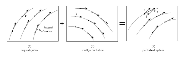
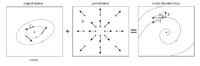
a) b) c)

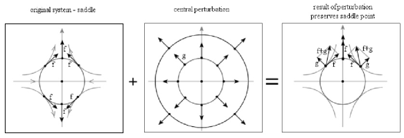
Figure 1: Illustration of the structural instability of center and (b) structural stability of saddle point. A perturbation of the original vector field $\boldsymbol{f}$ means the addition of a small vector $\boldsymbol{g}$. The effect of perturbation modifies it at every point in the state space (see (a)). The effect of adding a global perturbation to the original system disturbs a center point (see (b)) and preserves a saddle point as illustrated with figure (c).

The idea of structural stability attempts to define the notion of stability of differential deterministic models of physical processes.

For planar dynamical systems (as is the case for the models under consideration) Peixoto’s theorem Peixoto (1962) states that structurally stable dynamical systems form open and dense subsets in the space of all dynamical systems defined on the compact manifold. This theorem is a basic characterization of the structurally stable dynamical systems on the plane which offers the possibility of an exact definition of generic (typical) and non-generic (exceptional) cases (properties) employing the notion of structural stability. Unfortunately, there are no counterparts of this theorem in more dimensional cases when structurally unstable systems can also form open and dense subsets. For our aims it is important that Peixoto’s theorem can characterize generic cosmological models in terms of the potential function.

While there is no counterpart of Peixoto’s Theorem in higher dimensions, it is easy to test whether a planar polynomial system has a structurally stable global phase portrait. In particular, a vector field on the Poincaré sphere will be structurally unstable if there is a non-hyperbolic critical point at infinity or if there is a trajectory connecting saddles on the equator of the Poincaré sphere $S^{2}$. In opposite case if additionally the number of critical points and limit cycles is finite, $\boldsymbol{f}$ is structurally stable on $S^{2}$ (see (Perko, 1991, p. 322)). Following Peixoto’s theorem the structural stability is a generic property of the $C^{1}$ vector fields on a compact two-dimensional differentiable manifold $\mathcal{M}$.

Let us introduce the following definition

Definition 2

If the set of all vector fields $\boldsymbol{f}\in C^{r}(\mathcal{M})$ ($r\geq 1$) having a certain property contains an open dense subset of $C^{r}(\mathcal{M})$, then the property is called generic.

From the physical point of view it is interesting to known whether a certain subset $V$ of $C^{r}(\mathcal{M})$ (representing the class of cosmological accelerating models in our case) contains a dense subset because it means that this property (acceleration) is typical in $V$ (see Fig. 1).

It is not difficult to establish some simple relation between the geometry of the potential function and localization of the critical points and its character for the case of dynamical systems of the Newtonian type:

1. The critical points of the systems under consideration $\dot{x}=y$, $y=-\frac{\partial V}{\partial x}$ lie always on the $x$ axis, i.e. they represent static universes $y_{0}=0$, $x=x_{0}$;

2. The point $(x_{0},0)$ is a critical point of the Newtonian system iff it is a critical point of the potential function $V(x)$, i.e. $V(x)=E$ ($E$ is the total energy of the system $E=y^{2}/2+V(x)$; $E=0$ for the case of flat models and $E=-k/2$ in general);

3. If $(x_{0},0)$ is a strict local maximum of $V(x)$, it is a saddle type critical point;

4. If $(x_{0},0)$ is a strict local minimum of the analytic function $V(x)$, it is a center;

5. If $(x_{0},0)$ is a horizontal inflection point of the $V(x)$, it is a cusp;

6. The phase portraits of the Newtonian type systems have reflectional symmetry with respect to the $y$ axis, i.e. $x\to x$, $y\to-y$.

All these properties are simple consequences of the Hartman-Grobman theorem which states that near the non-degenerate critical points (hyperbolic) the original dynamical system is equivalent to its linear part. Therefore the character of a critical point is determined by the eigenvalues of the linearization matrix given by a simple equation $\lambda^{2}+\det{A}=0$, where

$$A=\left[\begin{array}[]{cc}0&1\\ -\frac{\partial^{2}V}{\partial x^{2}}&0\end{array}\right]_{(x_{0},0)}$$

is the linearization matrix. Hence, in the case of a maximum we obtain a saddle with $\lambda_{1}$, $\lambda_{2}$ real of opposite signs, and if the potential function assumes a minimum at the critical point we have a center with $\lambda_{1,2}$ purely imaginary of mutually conjugate. Therefore, among all distinguished cases, only if the potential function admits a local maximum at the critical point we have a structurally stable global phase portrait. Because $V\leq 0$ and $\partial V/\partial a=\frac{1}{6}(\rho+3p)(a)$ the Universe is decelerating if the strong energy condition is satisfied and accelerating if the strong energy condition is violated. Hence, among all simple scenarios, the one in which deceleration is followed by acceleration is the only structurally stable one (see Fig. 2).

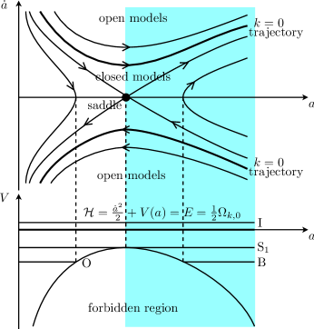
Figure 2: The model of an accelerating universe given in terms of the potential function and its phase portrait. The domain of acceleration is represented by shaded area. Note that only in this case with a single maximum of the potential function there are two phases of the universe evolution where the acceleration phase follows the deceleration phase. Note also, that the order of appearing of acceleration epochs is important and only in this case we obtain a structurally stable phase portrait. Therefore, from Peixoto’s theorem we obtain the generic phase portrait for the accelerating universe. It is equivalent to the $\Lambda$CDM model scenario.

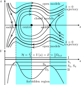
Figure 3: The model of an accelerating universe given in terms of the potential function and its phase portrait. The domain of acceleration is represented by shaded area. In this case the existence of two maxima induces the appearance of minima of the potential function whose presence gives rise to structural instability. Therefore, from Peixoto’s theorem we obtain the non-generic phase portrait for the universe accelerating in two domains.

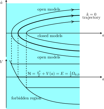
Figure 4: The model of an accelerating universe given in terms of the potential function and its phase portrait. The domain of acceleration is represented by shaded area. In this case the universe is accelerating for all trajectories. In the phase portrait there is no critical point in the finite domain. The potential function is decreasing function of the scale factor. While this system is structurally stable there is no matter dominating phase in the model. And from physical view of point is not interesting.

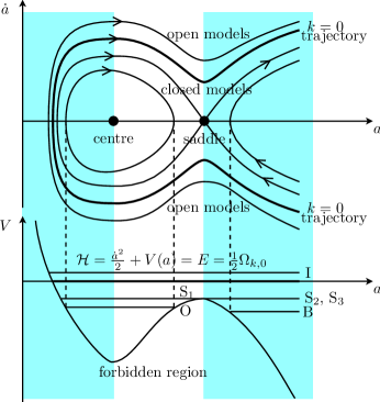
Figure 5: The model of an accelerating universe given in terms of the potential function and its phase portrait. The domain of acceleration is represented by shaded area. The phase portrait of extended bouncing models with the cosmological constant. While the early evolution is dominated by matter terms, for late times the cosmological term is dominating. There are three characteristic types of evolution: I – inflectional, O – oscillating, B – bouncing. The model is structurally unstable because of the presence of a non-hyperbolic critical point (center) on the phase portrait.

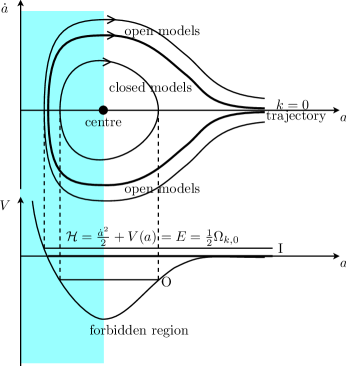
Figure 6: The model of an accelerating universe given in terms of the potential function and its phase portrait. The domain of acceleration is represented by shaded area. The phase portrait as well as the diagram of the corresponding potential for bouncing models $H^{2}/H_{0}^{2}=\Omega_{\text{m},0}x^{-m}-\Omega_{n,0}x^{-n}$, $n>m$, $m,n=\text{const}$. All trajectories represent cosmological models in which the phase of expansion is proceeded by the phase of contraction. They are closed for oscillating (O) models appearing for positive curvature, or open, representing bouncing flat and open cosmologies with a single bounce phase. On the phase portrait we find a single critical point of the center type. Because the presence of a critical point of non-hyperbolic type, the system is structurally unstable. The motion of the system is determined in the domain of the configuration space $V(a)<0$, i.e. for $a\geq a_{\text{min}}$ in the case presented on the figure. Note that for oscillating models there is an infinite number of transitions from acceleration to deceleration epoch. For flat and open cosmologies there is only one such transition.

Let us consider two types of scenarios of cosmological models with matter dominated and dark energy dominated phases

1. the $\Lambda$CDM scenario, where the early stage of evolution is dominated by both baryonic and dark matter, and late stages are described by the cosmological constant effects.

2. the bounce instead initial singularity squeezed into a cosmological scenario; one can distinguish cosmological models early bouncing phase of evolution (caused by the quantum bounce) Singh et al. (2006) from the classical bouncing models at which the expansion phase follows the contraction phase. In this paper by bouncing models we understand the models in the former sense (the modern one).

For the first class of models we obtain a global phase portrait equivalent to that which is demonstrated in Fig. 2. The eigenvalues of this system are real of opposite signs and this point is a saddle. It describes a stationary but unstable universe which is quite similar to the static Einstein Universe filled with both dust matter and with cosmological constant. There are, in principle, three representative scenarios of evolution. The trajectories moving in the region $B$ confined by the separatrices correspond to the closed universes contracting from the unstable de Sitter node towards the stable de Sitter node. They are sometimes called bouncing models (it is not the sense of bouncing models in the sense used by us in this paper – see Tables 1 and 2 for comparison). All trajectories on the phase plane are divided by a parabolic curve (representing the trajectory of the flat model) into two disjoint classes of closed and open models. The trajectory situated in the region $I$ confined by the upper branch of the trajectory $k=0$ and by the separatrices (coming out and approaching the saddle) of the saddle point, correspond to the closed universes expanding from the initial singularity ($x=0$, $\dot{x}=\infty$) to the stable deS₊ attractor. Quite similarly, the trajectories located in the symmetric region $x\to x$ and $y\to-y$ correspond to the closed contraction universes ($y<0$) from the unstable de Sitter node towards the singularity. The region $O$, whose boundaries are the separatrices coming out from the saddle and going to the saddle in the region $x\geq 0$, is covered by the trajectories of closed models which begins its expansion from the initial singularity, reach a maximal size and then recollapse to the final singularity. The trajectories situated over the upper branch of the trajectory of the flat model $k=0$ describe the open models expanding towards stable de Sitter universe from the initial singularity. They are called oscillating cosmological models.

The second class of models, described the cosmological models with a squeezing bounce phase in the cosmological scenario, is present in Fig. 3. Its phase portrait contains a center – non-hyperbolic critical point whose presence makes the system structurally unstable. Both phase portraits in Fig. 2 and 3 are topologically non-equivalent in the sense of existence of homeomorphism. In Fig. 4 we present a phase portraits of cosmological models with acceleration in all time; however there is no matter dominating phase during its evolution. In Fig. 5 it is presented a sub-case which starts with accelerating phase. This model is similar to the models considered in loop quantum cosmology which started with acceleration at very beginning.

In the simplest case we obtain a phase portrait equivalent to that presented on Fig. 6. Notice that all trajectories are bouncing and trajectories around the center are oscillating. The accelerating region is situated left of the critical point. In Fig. 5 the qualitative behaviour of the universes whose late time evolution is dominated by the cosmological constant term is presented. In this case we have two disjoint acceleration areas corresponding to that domain of configuration space at which the potential is a decreasing function of the scale factor.

One can imagine different evolutional scenarios in terms of the potential function (see Fig. 2-6). Because of the existence of a bouncing phase which always gives rise to the presence of a non-hyperbolic critical point on the phase portrait one can conclude

• the bounce is not a generic property of the evolutional scenario,

• structural stability prefers the simplest evolutional scenario in which the deceleration epoch is followed by the acceleration phase.

The dynamical systems with the property of such switching rate of expansion, following the single-well potential are generic in the class of all dynamical systems on the plane.

The presented approach to describe dynamics can be extended to the case of cosmological models with scalar field. They play an important role in the quintessence conception. To illustrate this let us consider a homogeneous, minimally coupled scalar field on the FRW background. The dynamical effects of this scalar field are equivalent to the effects of a perfect fluid with energy density and pressure given in the form

$$\begin{array}[]{l}\rho_{\phi}=\frac{1}{2}\varepsilon\dot{\phi}^{2}+U(\phi),\\ p_{\phi}=\frac{1}{2}\varepsilon\dot{\phi}^{2}-U(\phi),\end{array}$$

where $\varepsilon=+1$ for standard scalar field and $\varepsilon=-1$ for phantom scalar field, $U(\phi)$ is the potential of a scalar field.

A construction analogous to the presented above is to use the expression for the effective energy density. Let us consider for example a universe filled with perfect fluid with pressure $p=w\rho$, $w=\text{const}$ and a minimally coupled scalar field. Then, we can adopt the standard formula $V=-\frac{\rho_{\text{eff}}a^{2}}{6}$ (if we use conformal time $\mathrm{d}\eta=\mathrm{d}t/a$ then $V=-\frac{\rho_{\text{eff}}a^{4}}{6}$) and we obtain

$$V=-\frac{1}{6}\rho_{w,0}a^{-1-3w}-\frac{1}{6}\rho_{\phi}a^{2}.$$

After substituting $\rho_{\phi}$ into the above formula and the shifted kinetic term $-\frac{\varepsilon}{12}\phi^{2}$ into the kinetic energy of the system (remember that the division into the kinetic and potential parts has a purely conventional character), we obtain a $2$-dimensional Hamiltonian system in the form

$$\mathcal{H}=\frac{1}{2}\left(\frac{\mathrm{d}a}{\mathrm{d}t}\right)^{2}-\frac{1}{2}\varepsilon a^{2}\left(\frac{\mathrm{d}\phi}{\mathrm{d}t}\right)^{2}+\psi(a,\phi)\equiv-\frac{k}{2},$$ (10)

where in above formula we use units in which $8\pi G=c=1$ (some authors put $4\pi G/3=c=1$, then $V\equiv-\rho_{\text{eff}}a^{2}$), $\phi$ is a rescaled function $\phi\to\phi/\sqrt{6}$ and

$$\psi(a,\phi)=a^{2}U(\phi)+\frac{1}{6}\rho_{w,0}a^{1-3w}.$$

In the special case of the radiation filled universe ($w=1/3$) we obtain Hamiltonian system defined on the zero energy level

$$E\equiv-\frac{k}{2}+\frac{1}{6}\rho_{r,0}=\text{const}.$$

Therefore, in the case of potential $U(\phi)=\frac{1}{2}m^{2}\phi^{2}+\lambda\phi^{4}$ we obtain the $2$-dimensional potential function $\psi(a,\phi)$ which identify quintessence model. The same approach can be adopted to the case of conformally coupled scalar field a well as for complex scalar fields.

It is interesting to investigate what a class of quintessence models which reduces the dynamics of the universe with minimally coupled scalar field $\Phi$ (evolving in the potential $U(\Phi)$) to the dynamical system of a Newtonian type with the potential parameterized by the scale factor $V(a)$. The quintessence model is determined completely once the potential function $U$ of the scalar field is given. Thus energy density and pressure is given by

$$\rho_{\text{eff}}=-6\frac{V(a)}{a^{2}}.$$

On the other hand the dynamical system of a Newtonian type is specified completely once the potential $V(a)$ is fixed. Therefore if we assume that $\Phi=\Phi(a(t))$ then

$$\rho_{\Phi} =\frac{1}{2}\Phi^{\prime}(a)^{2}a^{2}H^{2}(a)+U(\Phi(a))$$

$$p_{\Phi} =\frac{1}{2}\Phi^{\prime}(a)^{2}a^{2}H^{2}(a)-U(\Phi(a))$$

and

$$w_{X}(a)=\frac{\Phi^{\prime}(a)^{2}a^{2}H^{2}(a)-2U(\Phi(a))}{\Phi^{\prime}(a)^{2}a^{2}H^{2}(a)+2U(\Phi(a))}$$

where $a^{2}H^{2}(a)=-2V(a)$.

Hence the particle-like approach can be extended naturally on the class of phenomenological quintessence models with the parameterized equation of state by redshift (or the scale factor equivalently) Linder (2003); Seljak et al. (2005). In this approach it is assumed the equation of state $p_{X}=w_{X}(a)\rho_{X}$ and $w_{X}=w_{X}(a)$ such that

$$\rho_{X}=\rho_{X,0}a^{-3(1+\bar{w}_{X}(a))}=\rho_{X,0}a^{-3}e^{\ln a^{-3\bar{w}_{X}(a)}}=\rho_{X,0}a^{-3}e^{-3\int_{1}^{a}w_{X}a^{-1}da}$$

where $\bar{w}_{X}(a)$ is the mean of the equation of state in the logarithmic scale, i.e.

$$\bar{w}_{X}(a)=\frac{\int w_{X}(a)d(\ln a)}{\int d\ln a}$$

The main motivation of the above assumption is the explanation of cosmic coincidence problem: why do all the contributions from the vacuum energy density (the cosmological constant) are comparable with energy density of matter? To remove the fine-tuning problem it was proposed a simple power law relation $\bar{w}_{X}(a)=w_{0}a^{\alpha}$, $w_{0},\alpha=\text{const}$ (scalling fluid) Rahvar and Movahed (2006). If we consider a scalar field parameterized by the scale factor, the class of possible quintessence paths is restricted from definition. Note that cosmography measures only average properties of matter expressed in kinematics of $H(z)$ and from (1) we obtain Guo et al. (2005)

$$\left(\frac{d\Phi}{dt}\right)^{2} =\rho_{X}(1+w_{X})$$ (11)

$$U(\Phi) =\frac{1}{2}\rho_{X}(1-w_{X})$$ (12)

where it is assumed that both the scalar field $\Phi$ and its potential $V(\Phi)$ depends on time through the scale factor, i.e. $\Phi(t)=\Phi(a(t))$, $U(\Phi(t))=U(\Phi(a))$. Then equation (11) can be rewritten to the new form

$$\left(\frac{d\Phi}{da}\right)^{2}=\frac{1}{a^{2}H^{2}}\rho_{X}(a)[1+w_{X}(a)]$$ (13)

or in terms of redshift $z$

$$\left(\frac{d\Phi}{dz}\right)^{2}=-\frac{\rho_{X}(z)[1+w_{X}]}{H^{2}(z)[1+z]^{2}}\quad\Longrightarrow\quad\Phi=\Phi(z)$$ (14)

where we use the standard relation $1+z=a^{-1}$ and $a_{0}=1$ is the value of the scale factor at present epoch. The potential $V$ in the dynamical system under consideration and the potential of the scalar field can be written as

$$V(a(z))=-\frac{a^{2}}{6}\left[\rho_{\text{m},0}a^{-3}+\rho_{X,0}a^{-3(1+\bar{w}_{X})}\right]$$ (15)

or

$$V(a(z))=-\frac{1}{6}\left[\rho_{\text{m},0}a^{-3}+\rho_{X,0}a^{-3}e^{-3\int_{1}^{a}w_{X}(a)d(\ln a)}\right]a^{2}$$ (16)

and

$$U(a)=\rho_{X,0}a^{-3}e^{-3\int_{1}^{a}w_{X}(a)d(\ln a)}(1-w_{X})$$ (17)

Hence

$$V(a)=-\frac{1}{6}\left[\rho_{\text{m},0}a^{-3}+(1-w_{X})^{-1}U(a)\right]a^{2}.$$ (18)

Let us return to the general Hamiltonian (10) then after substitution (13) to the potential $V=-\rho_{\text{eff}}a^{2}/6$, $\rho_{\text{eff}}=\rho_{\Phi}+\rho_{\text{m}}$

$$V =-\frac{1}{6}a^{2}\left[\frac{\rho_{X}(a)(1+w_{X}(a))}{2}+U(a)\right]-\frac{1}{6}\rho_{\text{m},0}a^{-1}=-\frac{1}{6}a^{2}\left[\frac{\rho_{X}(a)(1+w_{X}(a))}{2}+\frac{1}{2}\rho_{X}(1-w_{X})\right]-\frac{1}{6}\rho_{\text{m},0}a^{-1}$$

$$=-\frac{1}{6}\rho_{X}(a)a^{2}-\frac{1}{6}\rho_{\text{m},0}a^{-1}\equiv-\frac{1}{6}\rho_{\text{eff}}a^{2}$$ (19)

This means that after parameterization by the scale factor the scalar field quintessence model has the potential in the form just prescribed in the particle like description of quintessential models in which the phase space is two-dimensional instead of 4-dimensional ($\Phi,\dot{\Phi},a,\dot{a}$) Szydlowski and Czaja (2004a, b). Let us note that in this case the potential reconstruction performed by Rahvar and Mohaved is equivalent to the reconstruction of the corresponding potential function of the dynamical system $V(a)$. All dynamics is now squeezed to the plane $(a,\dot{a})$.

III The value of transition redshift and the Hubble parameter at the transition epoch

Due to the existence of a simple relation between the luminosity distance $d_{L}(z)$ as a function of redshift $z$ and the Hubble function

$$H(z)=\left[\frac{\mathrm{d}}{\mathrm{d}z}\left(\frac{d_{L}(z)}{1+z}\right)\right]^{-1},$$ (20)

it is possible to reconstruct the potential function $V(a)$. Note that even if the luminosity distance i obtained accurately the potential cannot be determined uniquely as it depends on $\Omega_{k,0}$ – an additional curvature parameter.

If we assume that the model is flat, then the trajectories of the corresponding Hamiltonian system lies on the zero energy level and

$$V(z)=-\frac{1}{2}\left\{(1+z)\frac{\mathrm{d}}{\mathrm{d}z}\left(\frac{d_{L}(z)}{1+z}\right)\right\}^{-2}.$$ (21)

The result of this reconstruction from the Riess sample is shown in Fig. 7. From this figure we obtain the shape of the potential function like the one of the $\Lambda$CDM model. Hence the corresponding phase portrait contains a single maximum. The value of redshift at this point we call the transition redshift and denote $z_{T}$. It is possible to obtain not only the qualitative shape of the potential function (an inverted single-well potential) but also some quantitative attributes of the model. Especially it is well to know when the switch from the deceleration to the acceleration epoch occurs in different cosmological scenarios. The result of fitting of the Newtonian type system with the simple potential function given in the simple polynomial form is presented in Table 2. From this estimation we obtain $z_{T}\simeq 0.5$ which can be interpreted as the value of redshift $z_{T}$ at which the switch between deceleration and acceleration epochs takes place.

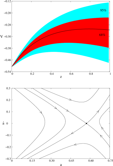
Figure 7: The potential function of the system reconstructed from SNIa data (the Riess et al. sample).

In Fig. 7 one can see that the universe is accelerating in the redshift interval in which the potential function decreases in respect to $z$. On the other hand the acceleration takes place in the region where the strong energy condition is violated. The idea of testing of energy condition through the measurement of distant SNIa was done by Santos et al. Santos et al. (2006).

Due to the particle like description dynamics of accelerating models one can also estimate the value of the Hubble function at the moment of the transition redshift, namely

$$H^{2}(z_{T})=-2(1+z_{T})^{2}H_{0}^{2}V(z_{T}).$$ (22)

From equation (22) we obtain that

$$H(z_{T})\simeq 0.9H_{0}.$$ (23)

There arises a basic problem in connection with the above coincidence: Why the value of $H(z_{T})$ and the present value of the Hubble function $H_{0}$ are of the same order of magnitude? The nature of this problem is similar to the cosmic coincidence conundrum Gorini et al. (2004).

From the definition of the potential function we can obtain a simple interpretation of acceleration of the Universe. For example, the deceleration parameter at the present epoch is the slope of the potential ($q_{0}=(\partial V/\partial a)_{a=1}$), jerk $j=\dddot{a}a^{2}/\dot{a}^{3}$ is related to the convexity of $V(x)\colon j_{0}=-(\partial V/\partial a^{2})_{a=1}$. Our results Szydlowski (2005); Szydlowski and Czaja (2005) also show the advantage of using $V(x)$ instead of the coefficient of the equation of state $w_{X}(z)$ to probe the variation of dark energy.

It have been recently shown the advantages of using $\rho_{X}(z)$ and $H(z)$, instead of the coefficient of equation of state Wang and Freese (2006); Wei and Zhang (2006). Note that both potential approaches are useful to differentiate between different dark energy propositions.

The potential function in the neighbourhood of its maximum can be approximated by

$$V(a)=V(a_{T})+\left(\frac{\mathrm{d}^{2}V}{\mathrm{d}a^{2}}\right)_{a_{T}}\frac{(a-a_{T})^{2}}{2}.$$

Hence we can calculate the energy density near the transition epoch $a=a_{T}$

$$\rho(a)=-\frac{6}{a^{2}}(a_{T}^{2}+V(a))\left(\frac{\mathrm{d}^{2}V}{\mathrm{d}a^{2}}\right)_{a_{T}}-3\left(\frac{\mathrm{d}^{2}V}{\mathrm{d}a^{2}}\right)_{a_{T}}+6\frac{a_{T}}{a}\left(\frac{\mathrm{d}^{2}V}{\mathrm{d}a^{2}}\right)_{a_{T}},$$

where $\left(\frac{\mathrm{d}^{2}V}{\mathrm{d}a^{2}}\right)_{a=a_{T}}=\frac{1}{6}a_{T}\frac{\mathrm{d}}{\mathrm{d}a}|_{a_{T}}(\rho+3p)$. The first and second terms are positive and correspond to $1$-dimensional topological defects and positive cosmological constant terms. The third term is negative and scales like $2$-dimensional topological defects.

It is useful to define space time metric of the non flat universe in the new variables

$$\mathrm{d}s^{2}=a^{2}\left\{\left[\frac{\mathrm{d}(\ln{a})}{\sqrt{-2V}}\right]^{2}-\mathrm{d}\Omega^{2}_{3}\right\}$$

or

$$\mathrm{d}s^{2}=a^{2}\left\{\mathrm{d}\tau^{2}-\mathrm{d}\Omega^{2}_{3}\right\},$$

where $\mathrm{d}\tau=\frac{\mathrm{d}(\ln{a})}{\sqrt{-2V}}$. Therefore, the only nontrivial metric function in a FRW cosmology is the function of $V(a)$ and the value of curvature which is encoded in the spatial part of the line element. Hence one can conclude any kind of observation based on geometry (cosmography) will allow us to determine a single potential function (for comparison see Padmanabhan (2003)). As argued by Padmanabhan, this function is insufficient to describe matter content of the universe and some additional input is still required.

Let us consider now the general properties of dark energy dynamics in terms of the potential. Due to particle-like description of cosmology with dark energy, the methods of qualitative analysis of differential equations can be naturally adopted. The main advantage of this method is the possibility of investigating all admissible evolutional paths for all initial conditions in the geometrical way – on the phase plane. The structure of the phase space is organized by singular solutions of the system which are represented by critical points (points of the phase plane for which right hand sides of the system vanishes) and phase curves connecting them. Following the Hartman-Grobman theorem the behaviour of the trajectories near the critical points is equivalent to the trajectories of linearized system at this point. Therefore for constructing of the picture of global dynamic called a phase portrait it is necessary to investigate all critical points and their type (determine the stability). The critical points $(x_{0},0)$ correspond to $y_{0}=0$ and $(\partial V/\partial x)_{x_{0}}=0$. They are saddle point if $V_{xx}(x_{0})<0$ and then eigenvalues of the linearization matrix $\lambda_{1,2}=\pm\sqrt{-V_{xx}(x_{0})}$ are real of opposite signs or centres if $V_{xx}(x_{0})>0$ and then eigenvalues are purely imaginary $\lambda_{1,2}=\pm i\sqrt{V_{xx}(x_{0})}$. The exceptional case of $V_{xx}(x_{0})=0$ is degenerate. Because only static critical point are admissible due to the constraint condition (Friedmann first integral) we obtain that $V(x_{0})=\frac{1}{2}\Omega_{k,0}$. Therefore, because $V(x)\leq 0$, the critical points are admissible for $\Omega_{k,0}\leq 0$, i.e. for the closed model only.

The system linearized around the critical point $x_{0}$ has the form

$$(x-x_{0})\dot{} =(y-0),$$ (24)

$$(y-y_{0})\dot{} =\left(-\frac{\partial^{2}V}{\partial x^{2}}\right)_{x=x_{0}}(x-x_{0}),$$ (25)

which is equivalent to a single differential equation of the second order

$$(x-x_{0})\ddot{}=\left(-\frac{\partial^{2}V}{\partial x^{2}}\right)_{x=x_{0}}(x-x_{0}).$$

The solution of the above linear system which approximates the behaviour of the trajectories near the critical point is

$$x-x_{0}=\frac{\dot{x}_{0}}{\sqrt{-(\partial^{2}V/\partial x^{2})_{x_{0}}}}\sinh{\sqrt{\left(-\frac{\partial^{2}V}{\partial x^{2}}\right)_{x_{0}}}(t-t_{0})},$$

where $x_{0}=x(t_{0})$ and $\dot{x}_{0}$ can be determined from the Friedmann first integral $\dot{x}_{0}=\sqrt{-2V(a_{0})}x_{0}$. The special choice $t_{0}=\pm\infty$ corresponds to the separatrices in and out-going from the static critical point.

Let us consider now the case of a saddle point. Then the angle of slopes of the separatrices at this point

$$\tan^{2}{\frac{\alpha}{2}}=-\left(\frac{\partial^{2}V}{\partial x^{2}}\right)_{x_{0}},$$

where $\alpha$ is the angle between eigenvectors at the critical point of the saddle type.

On the other hand from the reconstructed form of the potential function one can determine the dynamics on the phase plane without any information about the value of $\Omega_{k,0}$. Hence, we can establish the angle $\alpha$. It is strictly related to the value of jerk because of the relation $j_{0}=-(\partial^{2}V/\partial x^{2})_{x_{0}}$. Finally we obtain

$$\alpha=2\arctan{j_{0}}.$$

The universe is accelerating in such a domain of the configuration space in which $V(x)$ is a decreasing function of its argument. One can calculate the average value of time which trajectories spend during the loitering epoch ($\dot{a}$ close to zero)

$$\Delta t=\frac{1}{2x_{0}}\int^{x_{0}+\Delta x}_{x_{0}-\Delta x}\frac{x\mathrm{d}x}{\sqrt{-2V(X)}}=\frac{1}{2x_{0}}\int^{x_{0}+\Delta x}_{x_{0}-\Delta x}\frac{\mathrm{d}x}{H(x)},$$

where $x_{0}$ is the value of the scale factor at the transition epoch expressed in the units of its present value.

Hence the time which the model spends in the loitering epoch depends on the transition epoch ($z_{\text{tr}}$) and the preassumed value of $\Delta x$ – which measures deviation from this stage. For the FRW model with the $\Lambda$ term one can find exact forms of function $\Delta t(x_{0},\Delta x)$ in terms of the Jacobi elliptic functions.

IV The generic and non-generic global evolutional paths in the Multiverse of accelerating models

The analysis of full dynamical behaviour of trajectories requires the study of the behaviour of trajectories at infinity. It can be performed by means of the Poincaré sphere construction. In this approach we project the trajectories from center of the unit sphere $S^{2}=\{(X,Y,Z)\in\mathbf{R}^{3}\colon X^{2}+Y^{2}+Z^{2}=1\}$ onto the $(x,y)$ plane tangent to $S^{2}$ at either the north or south pole (see (Perko, 1991, p. 265)). Due to this central projection (introduced by Poincaré) the critical points at infinity are spread out along the equator. Therefore if we project the upper hemisphere $S^{2}$ onto the $(x,y)$ plane of dynamical system of the Newtonian type, then

$$x=\frac{X}{Z}\quad,\quad y=\frac{Y}{Z},$$ (26)

or

$$X=\frac{x}{\sqrt{1+x^{2}+\left(\frac{\partial V}{\partial x}\right)^{2}}},\quad Y=\frac{y}{\sqrt{1+x^{2}+\left(\frac{\partial V}{\partial x}\right)^{2}}},\quad Z=\frac{1}{\sqrt{1+x^{2}+\left(\frac{\partial V}{\partial x}\right)^{2}}}.$$ (27)

There is a simple way to introduce the metric in the space of all dynamical systems on the compactified plane.

If $\boldsymbol{f}\in C^{1}(\mathcal{M})$ where $\mathcal{M}$ is an open subset of $\mathbf{R}^{n}$, then the $C^{1}$ norm of $\boldsymbol{f}$ can be introduced in a standard way

$$\|\boldsymbol{f}\|_{1}=\sup_{x\in E}|\boldsymbol{f}(x)|+\sup_{x\in E}\|D\boldsymbol{f}(x)\|,$$ (28)

where $|\dots|$ and $\|\dots\|$ denotes the Euclidean norm in $\mathbf{R}^{n}$ and the usual norm of the Jacobi matrix $D\boldsymbol{f}(x)$, respectively.

It is well known that the set of vectors field bounded in the $C^{1}$ norm forms a Banach space (see (Perko, 1991, p. 312)).

It is natural to use the defined norm to measure the distance between any two dynamical systems of the multiverse. If we consider some compact subset $\mathcal{K}$ of $\mathcal{M}$ then the $C^{1}$ norm of vector field $\boldsymbol{f}$ on $\mathcal{K}$ can be defined as

$$\|\boldsymbol{f}\|_{1}=\max_{x\in\mathcal{K}}|\boldsymbol{f}(x)|+\max_{x\in\mathcal{K}}\|D\boldsymbol{f}(x)\|<\infty.$$ (29)

Let $E=\mathbf{R}^{n}$ then the $\varepsilon$-perturbation of $\boldsymbol{f}$ is the function $\boldsymbol{g}\in C^{1}(\mathcal{M})$ form which $\|\boldsymbol{f}-\boldsymbol{g}\|<\varepsilon$.

The introduced language is suitable to reformulate the idea of structural stability given by Andronov and Pontryagin. The intuition is that $\boldsymbol{f}$ should be structurally stable vector field if for any vector field $\boldsymbol{g}$ near $\boldsymbol{f}$, the vector fields $\boldsymbol{f}$ and $\boldsymbol{g}$ are topologically equivalent. A vector field $\boldsymbol{f}\in C^{1}(\mathcal{M})$ is said to be structurally stable if there is an $\varepsilon>0$ such that for all $\boldsymbol{g}\in C^{1}(\mathcal{M})$ with $\|\boldsymbol{f}-\boldsymbol{g}\|_{1}<\varepsilon$, $\boldsymbol{f}$ and $\boldsymbol{g}$ are topologically equivalent on open subsets of $\mathbf{R}^{n}$ called $\mathcal{M}$. Note that to show that system is not structurally stable on $\mathbf{R}^{n}$ it is sufficient to show that $\boldsymbol{f}$ is not structurally stable on some compact $\mathcal{K}$ with nonempty interior.

It was originally a wide spread opinion that structural stability was a typical attribute of any dynamical system modelling adequately a physical situation. The $2$-dimensional case is distinguished by the fact that Peixoto’s theorem gives the complete characterization of the structurally stable systems on any compact $2$-dimensional space and asserts that they form an open and dense subsets in the space of all dynamical systems on the plane.

Let us apply this framework to the multiverse of accelerating models represented in terms of a $2$-dimensional dynamical system of the Newtonian type on the Poincaré sphere $S^{2}$. Let the potential function be given in the polynomial form. If we assume that the coefficient of the equation of state can be expanded around the present epoch ($a=1$ or $z=0$) in the Taylor series, i.e.

$$\begin{array}[]{l}p_{X}=w_{X}(a)\rho_{X},\\ w_{X}(a)=\sum_{i=0}^{N}w_{i}(1-a)^{i},\end{array}$$ (30)

then we obtain from the conservation condition relation

$$\rho_{X}=\rho_{X,0}a^{-3(1+\sum_{i=0}^{N}(-1)^{i}w_{i})}\exp{\{3\sum_{k=0}^{N}(-1)^{k}\frac{(1-a)^{k}}{k}\sum_{i=k}^{N}(-1)^{i-k}w_{i}\}}.$$ (31)

Hence if we expand $\exp{\{\dots\}}$ in formula (31) then we obtain $\rho_{X}$ as well as $V(a)$ in the polynomial form

$$\rho_{X}=\rho_{X,0}a^{-3(1+\sum_{i=0}^{N}(-1)^{i}w_{i})}\left\{1+3\sum_{k=0}^{N}(-1)^{k}\frac{(1-a)^{k}}{k}\sum_{i=k}^{N}(-1)^{i-k}w_{i}+\frac{1}{2}\left[3\sum_{k=0}^{N}(-1)^{k}\frac{(1-a)^{k}}{k}\sum_{i=k}^{N}(-1)^{i-k}w_{i}\right]^{2}\right\}$$ (32)

and

$$V(a)=-\frac{\rho_{\text{m}}a^{2}}{6}-\frac{\rho_{X}a^{2}}{6}.$$ (33)

In the simplest case of $w(a)$ linearized around $a=1$ ($w=w_{0}+(1-a)w_{1}$), we obtain the density of dark energy

$$\rho_{X}=\rho_{X,0}a^{-3(1+w_{0}-w_{1})}\exp{[3w_{1}(a-1)]}=\rho_{X,0}a^{-3(1+w_{0}-w_{1})}\left\{1+3w_{1}(a-1)+9w_{1}^{2}(a-1)^{2}+\cdots\right\},$$ (34)

where $a^{-1}=1+z$, $x=a$, $a_{0}=1$.

If we consider some subclass of dark energy models described by the vector field $[y,-(\partial V/\partial x)]^{T}$ on the Poincaré sphere, then the right hand sides of the corresponding dynamical systems are of the polynomial form of degree $m$. Then $\boldsymbol{f}$ is structurally stable iff (i) the number of critical points and limit cycles is finite and each critical point is hyperbolic – therefore a saddle point in finite domain, (ii) there are no trajectories connecting saddle points. It is important that if the polynomial vector field $\boldsymbol{f}$ is structurally stable on the Poincaré sphere $S^{2}$ then the corresponding polynomial vector field $[y,-(\partial V/\partial x)]^{T}$ is structurally stable on $\mathbf{R}^{2}$ ((Perko, 1991, p. 322)). Following Peixoto’s theorem the structural stability is a generic property of $C^{1}$ vector fields on a compact two-dimensional differentiable manifold $\mathcal{M}$. If a vector field $\boldsymbol{f}\in C^{1}(\mathcal{M})$ is not structurally stable it belongs to the bifurcation set $C^{1}(\mathcal{M})$. For such systems their global phase portrait changes as vector field passes through a point in the bifurcation set.

Therefore, in the class of dynamical systems on the compact manifold, the structurally stable systems are typical (generic) whereas structurally unstable are rather exceptional. In science modelling, both types of systems are used. While the structurally stable models describe “stable configuration” structurally unstable model can describe fragile physical situation which require fine tuning Tavakol and Ellis (1988).

In Figs. 8, 9, 10 we show the phase portraits of different evolutional scenarios offered by different propositions of solving the cosmological problem. Among different models only the $\Lambda$CDM model (Fig. 8) (or phantom cosmology) and bouncing cosmology in Fig. 10a give rise to structurally stable evolutional paths.

The case of the phantom cosmology requires the additional comment. Let us consider the phantom cosmology with $w_{X}=4/3$ and dust matter. At the finite domain of the phase plane the system is described by

$$\dot{x} =y$$ (35a)

$$\dot{y} =-\frac{1}{2}\Omega_{\text{m},0}x^{-2}+\frac{3}{2}\Omega_{\text{ph},0}x^{2}$$ (35b)

and possesses the first integral in the form

$$\frac{1}{2}y^{2}+V(x)=\frac{1}{2}\Omega_{k,0}$$

where

$$V(x)=-\frac{1}{2}\Omega_{\text{m},0}x^{-1}-\frac{1}{2}\Omega_{\text{ph},0}x^{3}.$$

To investigate the behaviour of trajectories at infinity (i.e., on the circle at infinity $x^{2}+y^{2}=\infty^{2}$) it is useful to introduce the projective coordinates on the plane. There are two maps which cover the circle at infinity. Let us consider one of them

$$(x,y)\mapsto(v,w)\colon v=\frac{1}{y},w=\frac{x}{y}$$

Then the circle at infinity is covered by $y=0$, $-\infty<w<+\infty$ (for full investigation of the system the second map $(x,y)\mapsto(z,u)\colon z=\frac{1}{x},u=\frac{y}{x}$ should be studied and both coordinate systems are equivalent if $v\neq 0$ and $u\neq 0$).

In the coordinates $(v,w)$ system (35) assumes the form

$$\frac{dv}{d\eta} =\frac{1}{2}\left(\Omega_{\text{m},0}v^{5}-\Omega_{\text{ph},0}w^{4}v\right)$$ (36a)

$$\frac{dw}{d\eta} =\frac{1}{2}\Omega_{\text{m},0}v^{4}w-\frac{3}{2}w^{5}+vw^{2}$$ (36b)

where $dt/d\eta=vw^{2}$. Hence there is one (double) degenerated critical point situated at $x=0$, $y=\infty$.

The naïve thinking about the system gives rise to the supposition that the system is structurally unstable because of the existence of degenerated critical point in infinity. The objections are the following. All solutions of dynamical system $x(t,x_{0})$ can be divided on two categories – singular and non-singular. The former are represented by critical points in the phase space. The latter are visualized by trajectories joining them. While the trajectories at the finite domain of the phase space represent the physical evolution of the evolution, the trajectories at infinity are added to the model by the Poincaré sphere construction and they cannot represent the physical solution.

If we go along the trajectories in the future then at some moment of time, say $t=t_{\text{final}}$ become to tangent to the circle at infinity. This state is called the big-rip singularity. On the circle at infinity we can find a trajectory joining the big-rip singularity with the degenerate critical point $(x,y)=(0,+\infty)$. Note that this trajectory has no physical interpretation.

In the definition of structural stability itself it appears the assumption that the boundary of the domain at which the system is considered is a “cycle without contact”, i.e. there is a simple smooth curve $C$ which does not intersect the boundary. Although this assumption bounds a class of systems it makes this sense of notion of structural stability to be simpler Bautin and Leontovich (1976).

The parameterization of time, applied for establishing the qualitative equivalence of phantom model with the $\Lambda$CDM model, is not of course a diffeomorphism. However, the phantom system in the new parameterization can be treated as the model of physical reality. In this case the big-rip singularity is reached for infinity time due to reparametrization of time (see Fig. 9). In this case there is no non-physical trajectory lying on the circle in the infinity. This transformation prolongs incomplete trajectories to infinity and the big-rip singularity is a global attractor. From the physical point of view this parameterization of the phantom cosmology seems to be more adequate. Therefore, we claim that the phantom cosmology is structural stable. However, we must remember that the existence of topological equivalence of trajectories of the phantom and $\Lambda$CDM models does not mean their physical equivalence. It is manifested by the non-diffeomorphic reparameterization of time. It is an example that the scientific modelling we can use both the fragile and structurally stable models. But some of them seems to be more adequate of description of physical processes.

Figure 8: The phase portrait of the $\Lambda$CDM model on the projective phase plane $\mathbf{R}P^{2}$. Using the Poincaré sphere construction we represent the dynamics of $\Lambda$CDM models on the compactified plane with the circle at infinity. Note that critical points (hyperbolic) at infinity are structurally stable.

Figure 9: The phase portrait for phantom ($w_{X}<-1$) cosmology. The critical point at the circle $x=0$, $\dot{x}=\infty$ is degenerate but after redefinition of the positional variable $x\mapsto\bar{x}=x^{3/2}$ ($x\mapsto\bar{x}=x^{-(1+3w_{X})/2}$ in general) and then reparametrization of time following the rule $\tau\mapsto\eta\colon\frac{3}{2}\bar{x}^{1/3}\mathrm{d}\tau=\mathrm{d}\eta$, we obtain a “regularized” system for phantom cosmology which is topologically equivalent to that in Fig. 8. It is important for our aims that this physically equivalent dynamical system is typical in the multiverse.

a) b)

Figure 10: Extended bouncing model on the Poincaré sphere. It is structurally unstable because of the presence of the center (left figure) or structurally stable if this center disappear in the physically admissible domain (right figure).

The cosmological models with dynamics as presented in Fig. 10a describe for example models in which instead of the initial singularity there is a characteristic bouncing phase. There are different situations which realize this type of evolution: the cosmological models with spinning fluid Szydlowski and Krawiec (2004) or the metric affine gravity (MAG) inspired model Krawiec et al. (2005); Puetzfeld et al. (2005). All trajectories in Fig. 10a represent bouncing models.

The qualitative behaviour of extended bouncing models (see Table 1) with the cosmological constant is illustrated in Fig. 10b. Because of the presence of an additional center on the phase portrait the models lost the property of structural stability which is the attribute of the models in Fig. 10a. Therefore, they are non-generic in the multiverse. An analogous type of evolution appeared as a phenomenological implication of discreteness in Loop Quantum Cosmology Singh and Vandersloot (2005). In general, if we consider a squeezing bounce phase in an evolutional scenario, we obtain a fragile model which is structurally unstable.

Recently Ashtekhar (Loops’05 Conference presentation) suggested that quantum gravity (geometry) can serve as a bridge between vast space time regions which are classically unrelated, i.e. in Loop Quantum Gravity, singularity is a transitional phenomenon. Therefore, the resolution of the singularity problem of general relativity is replaced by approach to singularity with a bounce generated by quantum effects.

From our point of view such types of evolutional scenarios are not typical in the space of all evolutional paths on the plane.

Moreover, brane world models allow for a transient acceleration of the Universe which is preceded and followed by matter domination epoch (deceleration epoch). They admit so-called “quiescent” cosmological singularities Shtanov and Sahni (2002), at which the density, pressure and Hubble parameter remain finite, while all invariants of the Riemann tensor diverge to infinity within a finite interval of cosmic time. From our consideration such models are exceptional, i.e. while time-like extra dimension can avoid cosmological singularity by bounce this proposition is not generic in the multiverse.

The Sobolev metric introduced in the multiverse of dark energy models can be used to measure how far different cosmological model with dark energy are to the canonical $\Lambda$CDM model. For this aim let us consider a different dark energy models with dust matter and dark energy. We also for simplicity of presentation assume for all models have the same value of $\Omega_{\text{m},0}$ parameters which can be obtained, for example, from independent extragalactic measurements. Then, the distance between any two cosmological model, say model “1” and model “2” is

$$d(1,2)=\max_{x\in C}\{|V_{1x}-V_{2x}|,|V_{1xx}-V_{2xx}|\},$$

where we assumed the same value of the $H_{0}$ parameter measured at the present epoch for all cosmological models which we compare, $V_{1}$ and $V_{2}$ and their derivatives are only the parts of the potentials without the matter term.

Because $(V_{1}-V_{2})_{x}$ measures the difference of slopes at any $x$, the distance $d$ in general becomes a function of $x$. However, for fitting or constraining a model’s parameters we use actual observational data obtained at $x=1$ epoch. Therefore, a closed region $C$ on which we compare predictions of different theoretical models can be chosen such that $C=\{1\}\times\{y\colon 0<y\leq\sqrt{-2V(1)},V(1)=-1/2\}$. Of course, it is a closed domain. From the definition of the metric $d$, two models are close if the slopes of tangents at the present epoch are close. This metric can also be expressed in dimensionless parameters, then we simply obtain the deceleration parameter instead of slopes. Also, instead of $C^{1}$ metric $C^{r}$ metric can be defined. Then $C^{r}$ metric measures the distance between any two models more precisely by comparing their additional acceleration indicators like jerk, snap, crackle or higher derivatives of potential functions. In general, the metric is a function of the model’s parameters. Therefore with estimating the values of parameters, one can immediately determine the distance between any two models – elements of an ensemble of dark energy models. Because at present we can only measure the second derivative of scale factor as an acceleration indicator, $C^{1}$ metric seems to be sufficient to order variety of dark energy models for answering how far the model is from the $\Lambda$CDM one and any other. In this way we obtain a ranking of cosmological models from the point of view of closeness to the concordance $\Lambda$CDM model. Different models belong to the open ball at the center of which the $\Lambda$CDM model is located. One can show the existence of the following inclusion relation Szydlowski and Kurek (2006a); Szydlowski and Krawiec (2006)

$$S_{\Lambda\text{CDM}}\subset S^{(w_{X}\text{fitted})}_{\text{phantom}}\subset S^{w_{X}=-4/3}_{\text{phantom}}\subset S_{\text{Cardassian}}\cdots$$

It is interesting that the above ordering is correlated with one obtained from the Bayesian information criterion Szydlowski and Kurek (2006b); Szydlowski et al. (2006).

V Conclusions

The main goal of this paper was to investigate the structure of the space of all FRW models which offer the possibility of explaining SN Ia data. To this aim we presented a unified language of dynamical systems of the Newtonian type in which the potential function determines all properties of the system. We defined the space of all dynamical systems, called the multiverse, of accelerating models. This space can be naturally equipped with the structure of Banach space which measures the distance between two models. This metric can be used to measure how far different model are from the concordance $\Lambda$CDM model.

The complexity of different models can be defined in terms of the potential function. This function determines the domains of the configuration space in which the Universe accelerates or decelerates. The concept of structural stability was used to distinguish generic models in the multiverse. Following Peixoto’s theorem we called them typical in the multiverse because they form open and dense subsets. The structurally unstable models are exceptional and form sets of zero measure in the multiverse. Our main result is that the structural stability property uniquely determines the shape of the potential. It is shown that genericity favours inverted single-well shape of the potential function.

On the other hand, this function could be reconstructed (modulo curvature) from distant type Ia supernovae data and the obtained function is equivalent to the potential function for the $\Lambda$CDM model. The evolutional scenario in which the acceleration epoch is proceeded by deceleration is uniquely distinguished. Therefore, while different theoretically allowed evolutional scenarios have been proposed and formulated in terms of the potential function, the simplicity of the evolutional scenario is the best guide to our Universe – the inverted single-well potential function is preferred. In other words, our Universe shows evidence of complexity and at the same time great simplicity which allows us to probe its properties with the help of simple models.

In explanation and understanding of the observational data we use the models (an idea of cosmological models). However, between the physical subjects and theoretical notions there is a 1–1 correspondence preserving some relations (isomorphism).

If we require the property of structural stability of the model we implicitly apply what McMullin called cosmogonic indifference principle McMullin (1993). While the anthropic like principles concentrated on explaining some properties of the Universe by the specially chosen model parameter, initial conditions or laws of physics, the indifference type of explanation concentrate on searching upon very generic initial conditions and laws of physics which act to produce the special configuration (see (Stoeger et al., 2004, p. 18)). Stoeger, Ellis and Kirchner argue that indifference principle is more interesting from the physical point of view relative to anthropic type of explanation which is more useful in philosophy. The authors claim that the problem of choosing between two principles: special or generic model has a rather philosophical (or epistemological) character to which the interpretation of our results is strictly related.

Therefore if we concentrate on searching for a very generic class of dark energy models or modification of the FRW equation that produce the special configuration we now enjoy – an accelerating Universe, then the postulate of structural stability naturally gives rise to such a situation.

A natural question is whether the inverted single-well potential is favoured over other more complex models with double, triple etc. accelerating phases. This can be addressed by using the Bayesian information criteria (BIC) of model selection. Our analysis confirms that there is no strong reason for inclusion of extra complexity (more accelerating epochs) and the model with a single acceleration epoch is favoured over the others by supernovae data Godlowski and Szydlowski (2005); Szydlowski et al. (2005).

Different conclusions can be made from our analysis but the answer to the question put in the title seems to be especially tempting. We are living in an accelerating Universe because simplicity is the best guide to our Universe. Moreover, because our Universe is typical (generic) and its model can be discovered by using the approximation method starting from a simple (possibly naive) model – the $\Lambda$CDM (or phantoms).