Evidence for the importance of resonance scattering in X-ray emission line profiles of the O star $\zeta$ Puppis

Abstract

We fit the Doppler profiles of the He-like triplet complexes of O VII and N VI in the X-ray spectrum of the O star $\zeta$ Pup, using XMM-Newton  RGS data collected over $\sim 400$ ks of exposure. We find that they cannot be well fit if the resonance and intercombination lines are constrained to have the same profile shape. However, a significantly better fit is achieved with a model incorporating the effects of resonance scattering, which causes the resonance line to become more symmetric than the intercombination line for a given characteristic continuum optical depth $\tau_{*}$. We discuss the plausibility of this hypothesis, as well as its significance for our understanding of Doppler profiles of X-ray emission lines in O stars.

1 Introduction

High resolution X-ray spectra obtained with diffraction grating spectrometers on the Chandra and XMM-Newton  X-ray observatories have revolutionized our understanding of the X-ray emission of O stars in the last five years. In the canonical picture, the X-rays are emitted in plasmas heated by shocks distributed throughout the wind (Cassinelli & Swank, 1983; Corcoran et al., 1993, 1994; Hillier et al., 1993); the shocks are created by instabilities in the radiative driving force (e.g. Lucy & White, 1980; Owocki et al., 1988; Cooper, 1994; Feldmeier et al., 1997). Although some stars show anomalous X-ray emission that can be explained by a hybrid mechanism involving winds channelled by magnetic fields (e.g. $\tau$ Sco and $\theta^{1}$ Ori C, Donati et al., 2002, 2006; Cohen et al., 2003; Gagné et al., 2005), a number of “normal” O stars have X-ray spectra that are mostly consistent with the wind-shock paradigm (e.g. $\zeta$ Pup, $\zeta$ Ori, and $\delta$ Ori). The papers describing the first few high resolution spectra of normal O stars obtained reported some inconsistencies with expectations (Waldron & Cassinelli, 2001; Kahn et al., 2001; Cassinelli et al., 2001; Miller et al., 2002; Waldron et al., 2004), but more recent quantitative work based on the simple empirical Doppler profile model of Owocki & Cohen (2001, hereafter OC01) has resolved many of these problems (Kramer et al. 2003; Cohen et al. 2006; Leutenegger et al. 2006). The main outstanding problem is the relative lack of asymmetry in emission line Doppler profiles, which, if taken at face value, would imply reductions in the literature mass-loss rates of an order of magnitude (Kramer et al., 2003; Cohen et al., 2006; Owocki & Cohen, 2006).

Although there is mounting evidence from other lines of inquiry suggesting that the literature mass-loss rates may be systematically too high (Massa et al. 2003; Hillier et al. 2003; Bouret et al. 2005; Fullerton et al. 2006), there are also subtle radiative transfer effects that could cause emission line profiles to be more symmetric than one might naively expect. Two effects that have been investigated in the literature are porosity (Feldmeier et al., 2003; Oskinova et al., 2004, 2006; Owocki & Cohen, 2006) and resonance scattering (Ignace & Gayley, 2002, hereafter IG02). Porosity could lower the effective opacity of the wind to X-rays, thus symmetrizing emission lines. However, Oskinova et al. (2006) and Owocki & Cohen (2006) have found that the characteristic separation scale of clumps must be very large to show an appreciable effect on line profile shapes, which makes it difficult to achieve a significant porosity effect. Resonance scattering can symmetrize Doppler profiles by favoring lateral over radial escape of photons; it is an intriguing possibility, but to date it has not been tested experimentally.

In this paper, we present evidence for the importance of resonance scattering in some of the X-ray emission lines in the spectrum of the O star $\zeta$ Pup. We show that the blend of resonance and intercombination lines of two helium-like triplets in the very high signal-to-noise ratio XMM-Newton  Reflection Grating Spectrometer (RGS) spectrum of $\zeta$ Pup cannot be well fit by assuming that both lines have the same profile but can be much better fit by assuming the profile of the resonance line is symmetrized by resonance scattering.

This paper is organized as follows: in § 2 we discuss the reduction of over 400 ks of XMM-Newton  RGS exposure on $\zeta$ Pup; in § 3 we briefly recapitulate the results of OC01 and Leutenegger et al. (2006) for Doppler profile modelling (§ 3.1), and we show that the He-like OC01 profile model does not give a good fit to the O VII and N VI triplets of $\zeta$ Pup (§ 3.2); in § 4 we generalize the results of OC01 to include the effects of resonance scattering as derived in IG02 (§ 4.1), and we fit this model to the data (§ 4.2); in § 5 we discuss our results; and in § 6 we give our conclusions.

2 Data reduction

The data were acquired in 11 separate pointings. The first two observations were performance verification, while the rest were calibration; they are all available in the public archive. The ODFs were processed with SAS version 7.0.0 using standard procedures; periods of high background were filtered out. Only RGS (den Herder et al., 2001) data were used in this paper, but EPIC data are available for most of the observations. Processing resulted in a co-added total of 415 ks of exposure in RGS1 and 412 ks in RGS2. The observation IDs used and net exposure times are given in Table 1.

RGS has random systematic wavelength scale errors with a $1\sigma$ value of $\pm 7$ mÅ (den Herder et al., 2001). A 7 mÅ shift could lead to significant systematic errors in the model parameters measured from a line profile. Because of this, we co-add all observations using the SAS task rgscombine. Assuming the systematic shifts are randomly distributed, co-adding the data will result in a spectrum that is almost unshifted (depending on the particular distribution of shifts of the individual observations), but that is broadened by 7 mÅ; this effect is much easier to account for in our analysis. We have assumed that the data do not vary intrinsically. We have not formally verified that the data show no significant intrinsic variation, but upon visual inspection the data do not appear to vary more than expected from statistical fluctuations combined with the aforementioned random systematic errors in the wavelength scale.

Spectral fitting was done with XSPEC version 12.2.1; the line profile models are implemented as local models. The $C$ statistic (Cash, 1979) is used instead of $\chi^{2}$ because of the low number of counts per bin in the wings of the profiles.

Because of the failed CCD on RGS2, we only have RGS1 data for O VII He$\alpha$. We only fit RGS2 data for N VI He$\alpha$ because the complex falls on a chip gap for RGS1.

For each complex we fit, we first measured a local continuum strength from a nearby part of the spectrum uncontaminated by spectral features. We modeled this continuum as a power law with an index of 2, which is flat when plotted against wavelength. When fitting a line profile, we fit a combination of the local continuum (fixed to the measured value) plus the line profile model to the data.

For the N VI He$\alpha$ complex, we also included emission from C VI Ly$\beta$ at 28.4656 Å, since the red wing of this line overlaps the blue wing of the resonance line of N VI He$\alpha$. The model parameters for C VI Ly$\beta$ are assumed to be the same as for N VI, and it is assumed to be optically thin to resonance scattering.

Emission lines and complexes were fit over a wavelength range of $\lambda_{-}<\lambda<\lambda_{+}$. Here $\lambda_{\pm}=\lambda_{0}(1\pm v_{\infty}/c)\pm\Delta\lambda$, where $\Delta\lambda$ is the resolution of RGS at that wavelength. $\lambda_{0}$ is the shortest wavelength in the complex for $\lambda_{-}$ and the longest wavelength for $\lambda_{+}$.

3 Best fit He-like profile model

3.1 The profile model

In this section we briefly recapitulate the results of OC01 for the Doppler profile of an X-ray emission line from an O star wind and the extension of these results to a He-like triplet complex by Leutenegger et al. (2006).

In the physical picture of the OC01 model, the wind is a two-component fluid; the bulk of the wind is relatively cool material of the order of the photospheric temperature, while a small fraction of the wind is at temperatures of order 1–5 MK, so that it emits X-rays. The cool part of the wind has some continuum opacity to X-rays and can absorb them as they leave the wind.

The OC01 formalism casts the line profile in terms of a volume integral over the emissivity, attenuated by continuum absorption:

$$L_{\lambda}=4\pi\int dV\eta_{\lambda}(\mu,r)e^{-\tau_{c}(\mu,r)}$$ (1)

where $\eta_{\lambda}(\mu,r)$ is the emissivity at the observed wavelength $\lambda$ and $\tau_{c}(\mu,r)$ is the continuum optical depth to X-rays of the wind.

The line profile can be expressed in terms of the scaled wavelength $x\equiv(\lambda/\lambda_{0}-1)c/v_{\infty}=-v_{z}/v_{\infty}$; this gives the shift from line center in the observer’s frame in units of the wind terminal velocity. The sign convention is such that positive $x$ corresponds to a redshift.

OC01 derive an expression for the line profile in terms of an integral over the inverse radial coordinate $u=R_{*}/r$ [cf. their eqn. (9)]:

$$L_{x}=L_{0}\int_{0}^{u_{x}}\,du\,\left.\frac{f_{X}(u)}{w^{3}(u)}e^{-\tau(\mu,u)}\right|_{\mu=-x/w(u)}.$$ (2)

In this equation we have used the following expressions: $w(u)\equiv v(u)/v_{\infty}=(1-u)^{\beta}$ is the scaled velocity, $\tau(x,u)$ is the (continuum) optical depth to X-rays emitted along a ray to the observer, $f_{X}(u)\propto u^{q}$ is the filling factor of X-ray emitting plasma, and $u_{x}\equiv\min(u_{0},1-|x|^{1/\beta})$ is the upper limit to the integral; $u_{0}=R_{*}/R_{0}$ is the inverse of the minimum radius of X-ray emission $R_{0}$, and $1-|x|^{1/\beta}$ is a geometrical cutoff for the minimum radius that emits for a given value of $x$. The integral for $L_{x}$ can be evaluated numerically.

The optical depth in this expression is derived in OC01. It is written as the product of the characteristic optical depth $\tau_{*}=\kappa\dot{M}/4\pi R_{*}v_{\infty}$ times a dimensionless integral containing only terms depending on the geometry. It can be evaluated analytically for integer values of $\beta$. For non-integer values of $\beta$, the optical depth must be evaluated numerically, which is computationally costly, and thus not convenient in conjunction with the radial integral of the line profile. Because of this we assume $\beta=1$ throughout this paper, which is a good approximation for $\zeta$ Pup, as well as for O stars in general.

The interesting free parameters of this model are the exponent of the radial dependence of the X-ray filling factor, $q$; the characteristic optical depth to X-rays of the cold plasma, $\tau_{*}$; and the minimum radius for the onset of X-ray emission $R_{0}$.

Leutenegger et al. (2006) extend this analysis to a He-like triplet complex. The only difference is that the forbidden-to-intercombination line ratio has a radial dependence due to photoexcitation of the metastable upper level of the forbidden line:

$${\cal R}\equiv\frac{f}{i}={\cal R}_{0}\frac{1}{1+\phi/\phi_{c}}={\cal R}_{0}\frac{1}{1+2PW(r)}.$$ (3)

Here $\phi$ is the photoexcitation rate from the upper level of the forbidden line; it depends on the photospheric UV flux and scales with the geometrical dilution $W(r)$; $\phi_{*}$ is the photoexcitation rate near the photosphere, so that $\phi=2\phi_{*}W(r)$; $\phi_{c}$ is the critical photoexcitation rate, which is a parameter of the ion; and $P=\phi_{*}/\phi_{c}$ is a convenient dimensionless parameter that gives the relative strength of photoexcitation and decay to ground near the star such that ${\cal R}(R_{*})={\cal R}_{0}/(1+P)$. In this paper, we use values of $P$ calculated from TLUSTY stellar atmosphere models (Lanz & Hubeny, 2003) as described in Leutenegger et al. (2006). Values of ${\cal R}_{0}$ are taken from Porquet et al. (2001).

To modify the expressions for the forbidden and intercombination line profiles to account for this effect, the emissivity is multiplied by the normalized line ratio:

$$\eta_{f}(r)=\eta(r)\frac{{\cal R}(r)}{1+{\cal R}(r)}$$ (4)

$$\eta_{i}(r)=\eta(r)\frac{1}{1+{\cal R}(r)}.$$ (5)

3.2 Best fit model

In this section we model the Doppler profiles of the O VII and N VI He-like triplets with the He-like profile of Leutenegger et al. (2006) described in § 3.1. The forbidden line is very weak for these two ions, and the intercombination line profile predicted by the model is not very different from the resonance line profile. The main difference in the profile of the resonance and intercombination lines is that the extremes of the wings are somewhat weaker. This is because the $f/i$ ratio reverts to the low UV flux limit at very large radii ($>100R_{*}$ for O VIII for $\zeta$ Pup), so the intercombination line strength is reduced by a factor of a few. However, this has only a small effect on the profile shape.

Although it is weak, the predicted strength of the forbidden line is a good check on the consistency of the profile model. The value of the characteristic optical depth $\tau_{*}$ can have a strong effect on the observed $f/i$ ratio by setting the value of $R_{1}$, the radius of optical depth unity. However, this effect is degenerate with the value of $q$, the exponent of the radial dependence of the X-ray filling factor.

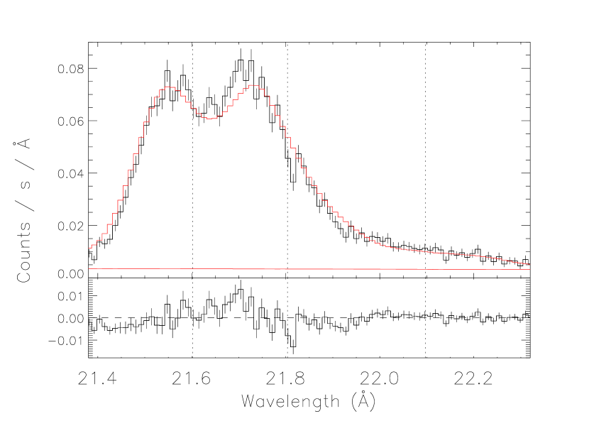
Figure 1: O VII triplet with best-fit OC01 He-like triplet model (not including the effects of resonance scattering). The top panel shows the data in black with error bars and the model in red. The flat red line shows the assumed continuum strength. The bottom panel shows the fit residuals.

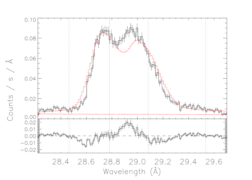
Figure 2: Same as Fig. 1, but for the N VI triplet. The C VI Ly$\alpha$ line at 28.4656 Å is also included in the fit, as well as the other fits to the N VI triplet.

In Figures 1 and 2, we show the Doppler profiles of the O VII and N VI He-like triplets, together with the best-fit models. The best-fit parameters are given in Tables 2 and 3. There are significant residuals in both fits. The N VI triplet shows stronger residuals than O VII. The residuals have a systematic shape: the model predicts a greater flux than the data on the blue wing of the resonance line and the red wing of the intercombination line, while it underpredicts the data in the center of the blend.

The systematic nature of the residuals shows that the shapes of the Doppler profiles of the resonance and intercombination lines are different. The residuals are consistent with the model resonance line being too blue and therefore too asymmetric, and the model intercombination line being too red and therefore too symmetric.

Resonance scattering has been proposed by IG02 as an explanation for the properties of O star X-ray emission line Doppler profiles. If it is important, it can cause significant symmetrization of profiles of strong resonance lines. Because this is in qualitative agreement with our observations, we explore this idea further.

4 Best-fit model including the effects of resonance scattering

4.1 Incorporating resonance scattering into OC01

The wind structure that gives rise to X-ray emission is likely to be extremely complex, with a highly nonmonotonic velocity field coupled to strong density variations in all three dimensions. Nonetheless, even in such a medium, the overall flow pattern, to first approximation, should still be largely dominated by the radial acceleration of a mostly radial, supersonic outflow. In such a medium, the radiative transfer of line emission can be well modelled in terms of localized escape methods first developed by Sobolev (1960), so we use this as our basis for investigating the possible role of resonance scattering in X-ray emission lines. Our approach here generally follows that taken by IG02, with two modest generalizations: (1) Instead of assuming a fully optically thick line, we allow the line optical depth to be a free parameter that can range from the optically thin to thick limits; and (2) instead of assuming a constant-speed expansion, we allow for a nonzero radial acceleration.

For a purely spherical expansion with radial velocity $v$ and radial velocity gradient $dv/dr$, let us first define an expansion anisotropy factor,

$$\sigma\equiv\frac{r}{v}\frac{\partial v}{\partial r}-1\,.$$ (6)

The Sobolev optical depth along a direction $\cos\,\mu$ can then be written in the form

$$\tau_{\mu}=\frac{\tau_{0}}{1+\sigma\mu^{2}}\,,$$ (7)

where $\tau_{0}$ is a characteristic optical depth in the lateral ($\mu=0$) direction [as defined further in eqn. (14) below]. The angle-dependent Sobolev escape probability is then given by

$$p(\mu)=\frac{1-e^{-\tau_{\mu}}}{\tau_{\mu}}\,.$$ (8)

For line photons trapped within a local Sobolev resonance layer, this represents the probability of escape per scattering. When normalized by the angle-averaged escape probability,

$$\left<p\right>\equiv\frac{1}{2}\int_{-1}^{1}p(\mu)\,d\mu\,,$$ (9)

then $p(\mu)/\left<p\right>$ gives the relative angle distribution of net line emission from a localized site of thermal photon creation.

To include the effects of resonance scattering on X-ray line emission, we can thus generalize the basic OC01 formalism, developed for the purely optically thin emission, by simply multiplying the local emissivity [cf. eqn. (2) or OC01 eqn. (9)] by this normalized angle distribution:

$$L_{x}=L_{0}\int^{u_{x}}_{0}du\frac{f_{X}(u)}{w^{3}(u)}\left[e^{-\tau_{c}(\mu,u)}\frac{p(\mu)}{\left<p\right>}\right]_{\mu=-x/w(u)}\,.$$ (10)

For optically thin lines ($\tau_{\mu}\ll 1$), the angle emission correction recovers the simple isotropic scaling $p(\mu)/\left<p\right>=1$, while for optically thick lines ($\tau_{\mu}\gg 1$), it takes the form

$$\frac{p(\mu)}{\left<p\right>}=\frac{1+\sigma\mu^{2}}{1+\sigma/3}\,.$$ (11)

The analysis by IG02 examines this case of optically thick line emission in a constant speed expansion, for which $dv/dr=0$ implies $\sigma=-1$ and thus

$$\frac{p(\mu)}{\left<p\right>}=\frac{3}{2}\,(1-\mu^{2})\,.$$ (12)

To allow for a non zero radial velocity gradient, let us use here a similar $\beta$-law velocity form to compute the anisotropy factor defined in eqn. (6),

$$\sigma=\frac{\beta_{\mathrm{Sob}}u}{1-u}-1\,.$$ (13)

Note that this is independent of the wind terminal speed and for a given radius depends only on the velocity index $\beta_{\mathrm{Sob}}$. Taking $\beta_{\mathrm{Sob}}=0$ recovers the constant expansion case $\sigma=-1$, while $\beta_{\mathrm{Sob}}>0$ gives $\sigma>-1$ at the lower radii ($u>0$), where the wind is still accelerating. Overall, the parameter $\beta_{\mathrm{Sob}}$ thus provides a convenient proxy for varying the relative importance of flow acceleration (compared to spherical divergence) in the local Sobolev escape scalings of the X-ray emission.

Our introduction here of a separate symbol, $\beta_{\mathrm{Sob}}$, for the velocity index relevant for Sobolev escape reflects the notion that in such a complex flow the local regions of X-ray emission need not always rigorously follow the global velocity of the bulk wind outflow. In particular, since the X-ray emitting material is generally too highly ionized to be directly driven by line-opacity, it might feasibly be better modeled as having a locally flat velocity gradient, $dv/dr=0$, which would then be represented by a velocity index $\beta_{\mathrm{Sob}}=0$ instead of the $\beta\approx 1$ used to model the overall wind outflow. On the other hand, it might also be that the X-ray emitting gas is hydrodynamically so tightly coupled to the mean wind that even on a local scale of resonance trapping, it too exhibits a similarly positive acceleration that is best represented by taking $\beta_{\mathrm{Sob}}=\beta=1$. In the line-fitting analysis below, we thus consider both these options.

Instead of the IG02 assumption of optically thick lines, our analysis also allows general parameterization of the line optical thickness, as set by the overall factor $\tau_{0}$ that gives the Sobolev optical depth in the lateral direction $\mu=0$. In terms of fundamental atomic parameters, this is given by

$$\tau_{0}=\frac{3}{8}\,\frac{\lambda}{r_{e}}\,\frac{c}{v}\,f_{i}\,n_{i}\,\sigma_{T}\,r.$$ (14)

Here $r_{e}$ is the classical electron radius, $\sigma_{T}$ is the Thomson cross section, $f_{i}$ is the oscillator strength of the transition, and $n_{i}$ is the ion density. Using the steady state mass loss rate $\dot{M}=4\pi\rho r^{2}v$ within the assumed $\beta$ velocity law, this can be recast in a form explicitly showing the dependence on inverse radius $u$,

$$\tau_{0}=\tau_{0,*}\frac{u}{w^{2}(u)}\,,$$ (15)

where we have defined a characteristic Sobolev optical depth,

$$\tau_{0,*}=\frac{\lambda r_{e}c\dot{M}}{4R_{*}v^{2}_{\infty}}\left(f_{i}\frac{n_{i}}{\rho}\right)\,.$$ (16)

The factor

$$\frac{n_{i}}{\rho}=\frac{n_{i}}{n_{e}}\,\frac{n_{e}}{\rho}=\frac{A_{i}\,q_{i}\,f_{X}}{\mu_{N}\,m_{p}}$$ (17)

gives the ratio of the ion number density to the mass density. Here $A_{i}$ is the abundance of the element relative to hydrogen, $q_{i}$ is the ion fraction, $f_{X}$ is the filling factor of X-ray emitting plasma, and $\mu_{N}m_{p}$ is the mean mass per particle. We take this ratio to be a constant with radius, although in principle the ion fraction and filling factor could vary.

In this paper, we take $\tau_{0,*}$ as a free parameter. For general values of the optical depth, the angle-averaged escape probability cannot be evaluated analytically. Fortunately, Castor (2004, pp.128–129) gives a computationally efficient approximation (attributed to G. Rybicki) that is accurate to $\sim 1.5\%$, so we use this approximation to calculate $\left<p\right>$ for finite values of $\tau_{0,*}$.

We have implemented this X-ray emission formalism as a local model in XSPEC. The Sobolev optical depth has angular and radial dependence as given by eqn. (7) and (15). The additional parameters added to the OC01 model are a switch to turn on or off completely optically thick scattering; the characteristic Sobolev optical depth $\tau_{0,*}$ (used when the completely optically thick switch is off); and the value of the velocity law exponent used in calculating $\sigma$, $\beta_{\mathrm{Sob}}$.

Figures 3 and 4 compare sample results for X-ray line profiles assuming various values of $\tau_{0,*}$ and $\beta_{\mathrm{Sob}}$. The overall trend is for higher values of $\tau_{0,*}$ and lower values of $\beta_{\mathrm{Sob}}$ to give more symmetric profiles. The trend of lower values of $\beta_{\mathrm{Sob}}$ to give more symmetric profiles is what one would expect; lowering $\beta_{\mathrm{Sob}}$ suppresses the effect of the flow acceleration in promoting radial photon escape, thus enhancing lateral escape an symmetrizing the profile.

4.2 Best-fit model including resonance scattering

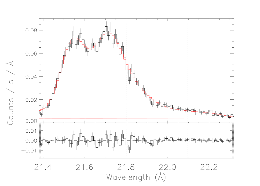
Figure 5: O VII triplet with best-fit model assuming resonance scattering with $\beta_{\mathrm{Sob}}=1$. Scheme is as in Fig. 1.

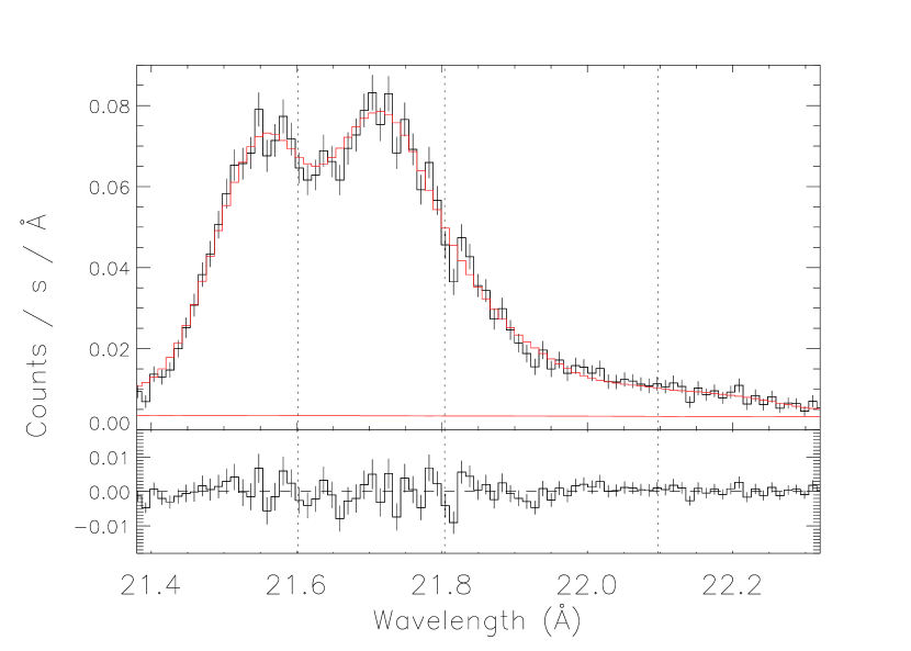
Figure 6: O VII triplet with best-fit model assuming resonance scattering with $\beta_{\mathrm{Sob}}=0$. Scheme is as in Fig. 1.

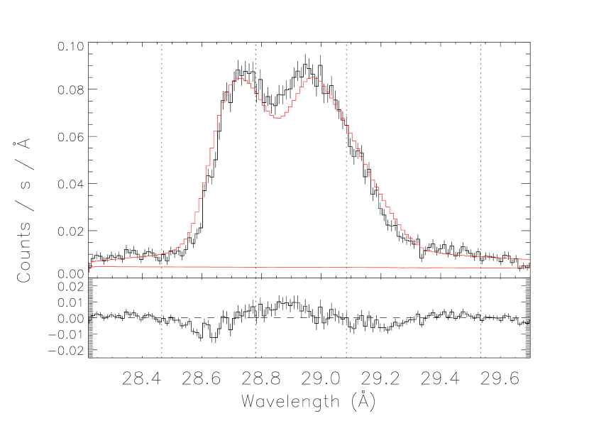
Figure 7: N VI triplet with best-fit model assuming resonance scattering with $\beta_{\mathrm{Sob}}=1$. Scheme is as in Fig. 1.

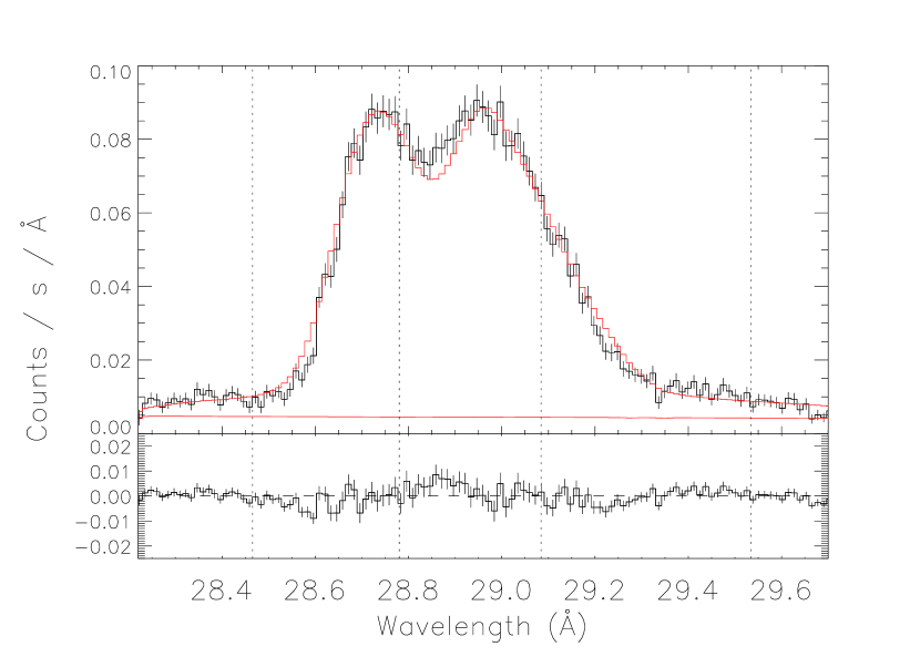
Figure 8: N VI triplet with best-fit model assuming resonance scattering with $\beta_{\mathrm{Sob}}=0$. Scheme is as in Fig. 1.

In this section we fit He-like profile models including resonance scattering to the O VII and N VI complexes. We fit each complex twice: once assuming $\beta_{\mathrm{Sob}}=1$ and once assuming $\beta_{\mathrm{Sob}}=0$. The best-fit models are shown in Figures 5, 6, 7, and 8. The best-fit parameters are given in Tables 2 and 3.

The O VII profile is well fit by either value of $\beta_{\mathrm{Sob}}$. We tested goodness of fit by comparing the fit statistic of 1000 Monte Carlo realizations of the model to the fit statistic of the data; both models are formally acceptable. The fit with $\beta_{\mathrm{Sob}}=1$ is better than that with $\beta_{\mathrm{Sob}}=0$ , but only by $\Delta C=3.8$, which is about $2\sigma$ for one interesting parameter. The fit with $\beta_{\mathrm{Sob}}=0$ has a significantly smaller value of $\tau_{0,*}$ than the fit with $\beta_{\mathrm{Sob}}=1$, as would be expected. The fit with $\beta_{\mathrm{Sob}}=1$ is statistically consistent with the approximation that the Sobolev optical depth becomes infinite.

The N VI profile is much better fit by either model including resonance scattering than it is by the original model. Furthermore, the model with $\beta_{\mathrm{Sob}}=0$ gives a significantly better fit than the model with $\beta_{\mathrm{Sob}}=1$. However, neither model is formally acceptable, and even the $\beta_{\mathrm{Sob}}=0$ model shows residuals of the same qualitative form as the original model, albeit of a much lower strength. For both models including resonance scattering, the optically thick approximation gives a better fit than a profile with finite Sobolev optical depth.

To test the significance of profile broadening introduced by co-adding data with random systematic errors in the wavelength scale, we have also fit each best-fit model with an additional 7 mÅ Gaussian broadening. In all cases, the best-fit parameters did not change significantly and the fit statistics were not significantly worse. Thus we conclude that our analysis is not strongly affected by this broadening.

5 Discussion

5.1 Comparison of results

The profile fits presented in § 3.2 clearly show that the O VII and N VI He-like triplet complexes in $\zeta$ Pup cannot be fit by models that assume the same profile shapes for the resonance and intercombination lines. The profile fits presented in § 4.2 show that these complexes can be much better fit by a model including the effects of resonance scattering.

However, although the O VII complex is well fit by a model including the effects of resonance scattering, the N VI complex shows differences in profile shape between the resonance and intercombination line that are greater than our model can reproduce, even under the most generous conditions ($\tau_{0,*}\rightarrow\infty,\beta_{\mathrm{Sob}}=0$). Furthermore, one would expect the two complexes to show relatively similar parameters; for example, since the elemental abundance of nitrogen appears to be roughly twice that of oxygen, one would expect the parameter $\tau_{0,*}$ to be about twice as large for the fit to N VI as it is for O VII. But a fit to the N VI profile with $\beta_{\mathrm{Sob}}=0$ and $\tau_{0,*}\approx 10$ (roughly twice the value measured for O VII) would give a substantially worse fit than a model with infinite Sobolev optical depth, which itself has significant residuals.

The fact that the apparent discrepancy between the shapes of the resonance and intercombination line profiles is much greater for N VI than for O VII implies that whatever the symmetrizing mechanism for the resonance line is, it is significantly stronger for N VI. There is no obvious explanation for this in the resonance scattering paradigm.

5.2 Plausibility of the importance of resonance scattering

It is worth revisiting the plausibility arguments of IG02 to confirm that one would expect resonance scattering to be important for these ions in the wind of $\zeta$ Pup. The relevant quantities to estimate are the Sobolev optical depth and the ratio of the Sobolev length to the cooling length.

The Sobolev length is given by (e.g. Gayley, 1995)

$$L_{\mu}=\frac{1+\sigma}{1+\sigma\mu^{2}}\frac{v_{\mathrm{th}}}{dv/dr}=\frac{v_{\mathrm{th}}}{v/r}\frac{1}{1+\sigma\mu^{2}}\,.$$ (18)

The cooling length is given by

$$\frac{5}{2}\frac{k\Delta T}{n_{e}\lambda}v,$$ (19)

as derived in IG02.

Taking the ratio,

$$\frac{L_{c}}{L_{\mu}} = \frac{5}{2}\frac{k\Delta T}{n_{e}\Lambda}\frac{v}{v_{th}}\frac{v}{r}(1+\sigma\mu^{2})$$ (20)

$$= \frac{5}{2}\frac{k\Delta T}{\Lambda}\frac{4\pi\mu_{N}m_{p}}{\dot{M}}\frac{v_{\infty}}{v_{th}}v_{\infty}^{2}R_{*}\frac{w^{3}(u)f_{X}}{u}(1+\sigma\mu^{2})$$ (21)

where we have used $\dot{M}=4\pi\mu_{N}m_{p}n_{e}r^{2}v$ for a smooth wind, and added a filling factor $f_{X}$ to correct for the ratio of the density of the X-ray emitting plasma to the mean density expected for a smooth wind.

Putting in some representative numbers appropriate to $\zeta$ Pup, we have

$$\frac{L_{c}}{L_{\mu}}=10\,(1+\sigma\mu^{2})\,\frac{w^{3}(u)f_{X}}{u}\,\frac{1}{\dot{M}_{6}}$$ (22)

where $\dot{M}_{6}$ is the mass-loss rate in units of $10^{-6}\,\mathrm{M_{\odot}\,yr^{-1}}$. We have used $\Lambda=6\times 10^{23}\,\mathrm{ergs\,s^{-1}\,cm^{3}}$, $\Delta T=2\mathrm{MK}$, $\mu_{N}=0.6$, $v_{th}=50\,\mathrm{km\,s^{-1}}$, $v_{\infty}=2500\,\mathrm{km\,s^{-1}}$, and $R_{*}=1.4\times 10^{12}\,\mathrm{cm}$.

This expression is greater than unity for lateral escape except at small radii ($r<2R_{*}$) if the filling factor is of order unity. However, if the filling factor is significantly less than unity, the Sobolev approximation may not be valid.

We now consider the expected values of the characteristic Sobolev optical depth,

$$\tau_{0,*}=\frac{\lambda\,r_{e}\,c\,\dot{M}}{4R_{*}\,v^{2}_{\infty}}\left(f_{i}\frac{n_{i}}{\rho}\right)=\frac{\lambda\,r_{e}\,c\,\dot{M}}{4\mu_{N}\,m_{p}\,R_{*}\,v^{2}_{\infty}}f_{i}\,A_{i}\,q_{i}\,f_{X}.$$ (23)

Putting in appropriate values, we get

$$\tau_{0,*}=120\,\left(f_{i}\,\frac{A_{i}}{10^{-3}}\frac{\lambda}{20\,\mbox{\AA}}\right)\,q_{i}\,f_{X}\,\dot{M}_{6}$$ (24)

We give calculations of $\tau_{0,*}/q_{i}f_{X}$ for important lines in O star spectra in Table 4. We have assumed solar abundances for all elements except C, N, and O (Anders & Grevesse, 1989). We assumed that the sum of CNO is equal to the solar value, with carbon being negligible and with nitrogen having twice the abundance of oxygen; this is an estimate based on the observed X-ray emission line strengths. Note that the Sobolev optical depth scales with the wavelength of the transition; this means that the Sobolev optical depths are significantly smaller for an X-ray transition than they are for a comparable UV transition. It also means that the longer wavelength K-shell transitions of N and O will be more strongly affected by resonance scattering than the shorter wavelength K-shell transitions of Ne, Mg, and Si, and L-shell transitions of Fe, a trend that is reinforced by the high elemental abundances of N and O.

Again, if the X-ray filling factors are of order unity, the characteristic Sobolev optical depths for the resonance lines of N VI and O VII are large, but X-ray filling factors of order $10^{-3}$ or less are sufficient to cause the lines to become optically thin. However, the requirement that the Sobolev length in the lateral direction be smaller than the cooling length is about as stringent, so if resonance scattering is important for strong lines, the Sobolev approximation should also be valid.

The high filling factors required are at odds with the simple two-component fluid picture of the OC01 model, since the X-ray filling factors are known to be very low. However, if we take the wind to be resolved into the two components on scales of the order of the Sobolev length, the filling factor would just be ratio of the local density to the mean density at that radius. This filling factor would still likely be less than unity for the X-ray emitting plasma, but not as low as the X-ray filling factor for the whole wind. This conjecture is a significantly stronger assumption than is made in OC01.

5.3 Impact of resonance scattering on Doppler profile model parameters

If resonance scattering is important in Doppler profile formation in the X-ray spectra of O stars, it may lead to a partial reconciliation with the literature mass-loss rates. The best-fit models for O VII have $\tau_{*}=4.1$, and the best-fit model for N VI has $\tau_{*}=3.0$. If we speculate that somehow the resonance line of N VI is even further symmetrized than predicted by our model, as the residuals in our best-fit model imply, the value of $\tau_{*}$ demanded by the intercombination line profile residuals should be somewhat higher; a reasonable guess would be $\tau_{*}\sim 4-5$.

These characteristic optical depths are higher than those measured by Kramer et al. (2003) for $\zeta$ Pup by applying the model of OC01 to Doppler profiles observed with the Chandra HETGS; the lines studied in that paper were mostly resonance lines as well. They are still somewhat lower than one would expect given the literature mass-loss rates; however, a detailed comparison with opacity calculations and mass-loss rates remains to be done. Furthermore, new, sophisticated analyses of UV absorption line profiles indicate that the published mass-loss rates of O star winds are too high (Massa et al., 2003; Hillier et al., 2003; Bouret et al., 2005); the most recent systematic analysis of Galactic O stars finds that for at least some spectral types, the published mass-loss rates must be at least an order of magnitude too great (Fullerton et al., 2006), but even the more conservative revisions lower the mass-loss rates by a factor of a few.

The fact that our measurements have $q\sim 0$ for both O VII and N VI is an important additional constraint. In cases in which one would like to fit a single emission line, it is desirable to have as few free parameters as possible. If we can assume $q=0$, we reduce the fitting of the profile shape to two free parameters for a line with no resonance scattering ($R_{0}$ and $\tau_{*}$) and three free parameters for a line with resonance scattering (the previous parameters in addition to $\tau_{0,*}$). Furthermore, for lines where $\tau_{*}$ is large enough to obscure the inner part of the wind, $R_{0}$ is effectively removed as a free parameter, further reducing the number of free parameters to one and two for non-resonance and resonance lines, respectively. Thus, high signal-to-noise ratio Doppler profiles with significant continuum absorption and no resonance scattering may provide robust measurements of the mass-loss rates of O stars. A good candidate for this is the 16.78 Å line of Fe XVII, which is likely not to be optically thick, and which is not blended with other lines.

5.4 Future work

Here we give a list of issues raised by this analysis that should be addressed in future work.

1. The discrepancies in the fits in this paper must be resolved. The fact that we cannot fit the N VI profile well is unsatisfactory. The difference between the appearance of the N VI complex and the O VII complex requires explanation.

2. The effect of resonance scattering on other resonance lines in the X-ray spectrum should be considered. Furthermore, unless we can make concrete predictions for the importance of resonance scattering for these lines, there may be significant fitting degeneracies between resonance scattering and low characteristic continuum optical depths.

3. The effect of multiple lines on resonance scattering should be explored. Of special importance is the calculation of the profile of a close doublet, such as Ly$\alpha$. In that case, the splitting between the two lines is of the order of the thermal velocity of the ions.

6 Conclusions

We have fit Doppler profile models based on the parametrized model of OC01 to the He-like triplet complexes of O VII and N VI in the high signal-to-noise ratio XMM-Newton  RGS X-ray spectrum of $\zeta$ Pup. We find that the complexes cannot be well fit by models assuming the same shape for the resonance and intercombination lines; the predicted resonance lines are too blue and the predicted intercombination lines are too red. This effect is what is predicted qualitatively if resonance scattering is important.

We find that models including the effects of resonance scattering give significantly better fits. However, there is significant disagreement between the O VII and N VI profiles in the degree of resonance line symmetrization that is difficult to understand in the framework of the resonance scattering model. Nevertheless, the general trend of the resonance scattering model to give more symmetrized profiles provides an interesting alternative (or supplement) to models that assume reduced wind attenuation due to reduced mass-loss rates and/or porosity.

Table 1: List of observations with net exposure times

	$t_{\mathrm{exp,RGS1}}$	$t_{\mathrm{exp,RGS2}}$
ObsID	(ks)	(ks)
0095810301	30.6	29.8
0095810401	39.7	38.3
0157160401	41.5	40.2
0157160501	32.8	32.8
0157160901	43.4	43.4
0157161101	27.0	27.0
0159360101	59.2	59.2
0159360301	22.0	22.0
0159360501	31.5	31.5
0159360901	46.6	46.6
0159361101	41.1	41.0

Table 2: Model fit parameters for O VII

Resonance
Scattering	$\beta_{\mathrm{Sob}}$	$q$	$\tau_{*}$	$u_{0}$	$\tau_{0,*}$	$G$	$n$	$C$	MC
No	$\cdots$	-0.21	1.6	0.62	$\cdots$	0.91	6.91	152.2	$\cdots$
Yes	1	$0.15^{+0.06}_{-0.07}$	$4.1^{+0.3}_{-0.4}$	$>0.68$	$>50$	$1.11^{+0.03}_{-0.04}$	$6.88\pm 0.07$	85.3	0.578
	0	$0.15\pm 0.07$	$4.1\pm 0.4$	$>0.63$	$5.9^{+3.2}_{-1.8}$	$1.02^{+0.04}_{-0.03}$	$6.88\pm 0.07$	89.1	0.730

Note. — The first row gives the best fit for a model not including resonance scattering (i.e. the model of OC01 and Leutenegger et al.). The second row gives the best fit for a model including resonance scattering with $\beta_{\mathrm{Sob}}=1$, and the last row has $\beta_{\mathrm{Sob}}=0$. We used a value of $P=1.67\times 10^{4}$ for all O VII profile models (Leutenegger et al., 2006).

Table 3: Model fit parameters for N VI

Resonance
Scattering	$\beta_{\mathrm{Sob}}$	$q$	$\tau_{*}$	$u_{0}$	$\tau_{0,*}$	$G$	$n$	$n_{\beta}$	$C$
No	$\cdots$	-0.34	0.5	0.58	$\cdots$	0.87	1.562	0	510.5
Yes	1	-0.09	2.1	0.50	thick	1.10	1.559	0.87	292.2
	0	0.06	3.0	0.48	thick	1.15	1.552	1.25	188.4

Note. — The first row gives the best fit for a model not including resonance scattering (i.e. the model of OC01 and Leutenegger et al.). The second row gives the best fit for a model including resonance scattering with $\beta_{\mathrm{Sob}}=1$, and the last row has $\beta_{\mathrm{Sob}}=0$. The C VI Ly$\beta$ line is assumed to have the same values of $q$, $\tau_{*}$, and $u_{0}$ as the N VI triplet, and is assumed not to be affected by resonance scattering. We used a value of $P=1.01\times 10^{5}$ for all N VI profile models (Leutenegger et al., 2006).

Table 4: Expected characteristic Sobolev optical depth

		$\lambda$	$f_{i}$	$A_{i}$	$\tau_{0,*}/q_{i}\,f_{X}$
Ion	Transition	(Å)		($10^{-3}$)
N VI	r	28.78	0.6599	0.9	103
	$\beta$	24.90	0.1478		20
N VII	Ly$\alpha$	24.78	0.1387, 0.2775		19, 37
O VII	r	21.60	0.6798	0.45	40
	$\beta$	18.63	0.1461		7
O VIII	Ly$\alpha$	18.97	0.1387, 0.2775		7, 14
Fe XVII		15.01	2.517	0.047	11
		15.26	0.5970		2.5
		16.78	0.1064		0.5
		17.05	0.1229		0.6
Ne IX	r	13.45	0.7210	0.12	7.0
	$\beta$	11.55	0.1490		1.2
Ne X	Ly$\alpha$	12.13	0.1382, 0.2761		1.2, 2.4
Mg XI	r	9.17	0.7450	0.038	1.6
Mg XII	Ly$\alpha$	8.42	0.1386, 0.2776		0.27, 0.53
Si XIII	r	6.65	0.7422	0.036	1.1
Si XIV	Ly$\alpha$	6.18	0.1386, 0.2776		0.19, 0.37

Figure 3: Comparison of the influence of different values of $\beta_{\mathrm{Sob}}$ on Doppler profile shape. All models have $q=0$, $u_{0}=\frac{2}{3}$, and $\tau_{*}=5$. The most asymmetric model is optically thin. Both of the other models use the approximation that $\tau_{0,*}$ is infinite; the more asymmetric of the two has $\beta_{\mathrm{Sob}}=1$, while the least asymmetric has $\beta_{\mathrm{Sob}}=0$.

Figure 4: Comparison of the influence of various values of the characteristic Sobolev optical depth $\tau_{0,*}$ on Doppler profile shape. All models have $q=0$, $u_{0}=\frac{2}{3}$, $\tau_{*}=5$, and $\beta_{\mathrm{Sob}}=0$. In order from most asymmetric to least, the models have $\tau_{0,*}=0,1,10,$ and $\infty$.

References

- Anders & Grevesse (1989) Anders, E. & Grevesse, N. 1989, Geochim. Cosmochim. Acta, 53, 197
- Bouret et al. (2005) Bouret, J.-C., Lanz, T., & Hillier, D. J. 2005, A&A, 438, 301
- Cash (1979) Cash, W. 1979, ApJ, 228, 939
- Cassinelli et al. (2001) Cassinelli, J. P., Miller, N. A., Waldron, W. L., MacFarlane, J. J., & Cohen, D. H. 2001, ApJ, 554, L55
- Cassinelli & Swank (1983) Cassinelli, J. P. & Swank, J. H. 1983, ApJ, 271, 681
- Castor (2004) Castor, J. I. 2004, Radiation Hydrodynamics (Radiation Hydrodynamics, by John I. Castor, pp. 368. ISBN 0521833094. Cambridge, UK: Cambridge University Press, November 2004.)
- Cohen et al. (2003) Cohen, D. H., de Messières, G. E., MacFarlane, J. J., Miller, N. A., Cassinelli, J. P., Owocki, S. P., & Liedahl, D. A. 2003, ApJ, 586, 495
- Cohen et al. (2006) Cohen, D. H., Leutenegger, M. A., Grizzard, K. T., Reed, C. L., Kramer, R. H., & Owocki, S. P. 2006, MNRAS, 368, 1905
- Cooper (1994) Cooper, R. G. 1994, Ph.D. Thesis
- Corcoran et al. (1993) Corcoran, M. F., Swank, J. H., Serlemitsos, P. J., Boldt, E., Petre, R., Marshall, F. E., Jahoda, K., Mushotzky, R., Szymkowiak, A., Arnaud, K., Smale, A. P., Weaver, K., & Holt, S. S. 1993, ApJ, 412, 792
- Corcoran et al. (1994) Corcoran, M. F., Waldron, W. L., Macfarlane, J. J., Chen, W., Pollock, A. M. T., Torii, K., Kitamoto, S., Miura, N., Egoshi, M., & Ohno, Y. 1994, ApJ, 436, L95
- den Herder et al. (2001) den Herder, J. W., Brinkman, A. C., Kahn, S. M., Branduardi-Raymont, G., Thomsen, K., Aarts, H., Audard, M., Bixler, J. V., den Boggende, A. J., Cottam, J., Decker, T., Dubbeldam, L., Erd, C., Goulooze, H., Güdel, M., Guttridge, P., Hailey, C. J., Janabi, K. A., Kaastra, J. S., de Korte, P. A. J., van Leeuwen, B. J., Mauche, C., McCalden, A. J., Mewe, R., Naber, A., Paerels, F. B., Peterson, J. R., Rasmussen, A. P., Rees, K., Sakelliou, I., Sako, M., Spodek, J., Stern, M., Tamura, T., Tandy, J., de Vries, C. P., Welch, S., & Zehnder, A. 2001, A&A, 365, L7
- Dere et al. (1997) Dere, K. P., Landi, E., Mason, H. E., Monsignori Fossi, B. C., & Young, P. R. 1997, A&AS, 125, 149
- Donati et al. (2002) Donati, J.-F., Babel, J., Harries, T. J., Howarth, I. D., Petit, P., & Semel, M. 2002, MNRAS, 333, 55
- Donati et al. (2006) Donati, J.-F., Howarth, I. D., Jardine, M. M., Petit, P., Catala, C., Landstreet, J. D., Bouret, J.-C., Alecian, E., Barnes, J. R., Forveille, T., Paletou, F., & Manset, N. 2006, MNRAS, 370, 629
- Feldmeier et al. (2003) Feldmeier, A., Oskinova, L., & Hamann, W.-R. 2003, A&A, 403, 217
- Feldmeier et al. (1997) Feldmeier, A., Puls, J., & Pauldrach, A. W. A. 1997, A&A, 322, 878
- Fullerton et al. (2006) Fullerton, A. W., Massa, D. L., & Prinja, R. K. 2006, ApJ, 637, 1025
- Gagné et al. (2005) Gagné, M., Oksala, M. E., Cohen, D. H., Tonnesen, S. K., ud-Doula, A., Owocki, S. P., Townsend, R. H. D., & MacFarlane, J. J. 2005, ApJ, 628, 986
- Gayley (1995) Gayley, K. G. 1995, ApJ, 454, 410
- Hillier et al. (1993) Hillier, D. J., Kudritzki, R. P., Pauldrach, A. W., Baade, D., Cassinelli, J. P., Puls, J., & Schmitt, J. H. M. M. 1993, A&A, 276, 117
- Hillier et al. (2003) Hillier, D. J., Lanz, T., Heap, S. R., Hubeny, I., Smith, L. J., Evans, C. J., Lennon, D. J., & Bouret, J. C. 2003, ApJ, 588, 1039
- Ignace & Gayley (2002) Ignace, R. & Gayley, K. G. 2002, ApJ, 568, 954
- Kahn et al. (2001) Kahn, S. M., Leutenegger, M. A., Cottam, J., Rauw, G., Vreux, J.-M., den Boggende, A. J. F., Mewe, R., & Güdel, M. 2001, A&A, 365, L312
- Kramer et al. (2003) Kramer, R. H., Cohen, D. H., & Owocki, S. P. 2003, ApJ, 592, 532
- Landi et al. (2006) Landi, E., Del Zanna, G., Young, P. R., Dere, K. P., Mason, H. E., & Landini, M. 2006, ApJS, 162, 261
- Lanz & Hubeny (2003) Lanz, T. & Hubeny, I. 2003, ApJS, 146, 417
- Leutenegger et al. (2006) Leutenegger, M. A., Paerels, F. B. S., Kahn, S. M., & Cohen, D. H. 2006, ApJ, in press
- Lucy & White (1980) Lucy, L. B. & White, R. L. 1980, ApJ, 241, 300
- Massa et al. (2003) Massa, D., Fullerton, A. W., Sonneborn, G., & Hutchings, J. B. 2003, ApJ, 586, 996
- Miller et al. (2002) Miller, N. A., Cassinelli, J. P., Waldron, W. L., MacFarlane, J. J., & Cohen, D. H. 2002, ApJ, 577, 951
- Oskinova et al. (2004) Oskinova, L. M., Feldmeier, A., & Hamann, W.-R. 2004, A&A, 422, 675
- Oskinova et al. (2006) —. 2006, MNRAS, submitted
- Owocki et al. (1988) Owocki, S. P., Castor, J. I., & Rybicki, G. B. 1988, ApJ, 335, 914
- Owocki & Cohen (2001) Owocki, S. P. & Cohen, D. H. 2001, ApJ, 559, 1108
- Owocki & Cohen (2006) —. 2006, ApJ, in press
- Porquet et al. (2001) Porquet, D., Mewe, R., Dubau, J., Raassen, A. J. J., & Kaastra, J. S. 2001, A&A, 376, 1113
- Sobolev (1960) Sobolev, V. V. 1960, Moving envelopes of stars (Cambridge: Harvard University Press, 1960)
- Waldron & Cassinelli (2001) Waldron, W. L. & Cassinelli, J. P. 2001, ApJ, 548, L45
- Waldron et al. (2004) Waldron, W. L., Cassinelli, J. P., Miller, N. A., MacFarlane, J. J., & Reiter, J. C. 2004, ApJ, 616, 542