Evolution of characteristic quantities for dark matter halo density profiles

Abstract

We have investigated the effect of an assembly history on the evolution of galactic dark matter (DM) halos of $10^{12}h^{-1}M_{\odot}$ using Constrained Realizations of random Gaussian fields. Five different realizations of a DM halo with distinct merging histories were constructed and have been evolved using collisionless high-resolution $N$-body simulations. Our main results are: A halo evolves via a sequence of quiescent phases of a slow mass accretion intermitted by violent episodes of major mergers. In the quiescent phases, the density is well fitted by an NFW profile, the inner scale radius $R_{\rm s}$ and the mass enclosed within it remain constant, and the virial radius ($R_{\rm vir}$) grows linearly with the expansion parameter $a$. Within each quiescent phase the concentration parameter ($c$) scales as $a$, and the mass accretion history ($M_{\rm vir}$) is well described by the Tasitsiomi et al. fitting formula. In the violent phases the halos are not in a virial dynamical equilibrium and both $R_{\rm s}$ and $R_{\rm vir}$ grow discontinuously. The violent episodes drive the halos from one NFW dynamical equilibrium to another. The final structure of a halo, including $c$, depends on the degree of violence of the major mergers and the number of violent events. Next, we find a distinct difference between the behavior of various NFW parameters taken as averages over an ensemble of halos and those of individual halos. Moreover, the simple scaling relations $c-$$M_{\rm vir}$ do not apply to the entire evolution of individual halos, and so is the common notion that late forming halos are less concentrated than early forming ones. The entire evolution of the halo cannot be fitted by single analytical expressions.

1. Introduction

The hierarchical buildup of cold dark matter (CDM) halos is a strongly nonlinear process. It is associated with the buildup of a unique density profile — one of the most fundamental characteristics of the DM halos. Based on $N$-body simulations, Navarro et al. (1997, hereafter NFW) found that the CDM halos can be universally fitted by a two-parameter functional form:

$$\rho(r)=\frac{4\rho_{\rm s}}{(r/R_{\rm s})(1+r/R_{\rm s})^{2}}\,,$$ (1)

where $R_{\rm s}$ is a characteristic “inner” radius at which the logarithmic density slope is $-2$ and $\rho_{\rm s}$ is the density at $R_{\rm s}$. The cosmological evolution of the NFW parameters, therefore, is an issue of a broad interest and is addressed in this work.

A useful alternative parameter to describe the shape of the profile is the so-called halo concentration parameter defined as $c=R_{\rm vir}/R_{\rm s}$, where $R_{\rm vir}$ is the halo virial radius. Although such a profile has been confirmed by numerous $N$-body simulations, the exact value of the inner slope parameter is uncertain. Several authors have found that halos have density cusps steeper (e.g., Fukushige & Makino, 1997, 2003; Moore et al., 1999; Ghigna et al., 2000) or shallower (e.g., Subramanian et al., 2000; Taylor & Navarro, 2001) than $-1$, the NFW value. The NFW profile and its modifications are specific cases of a three-parameter profile family proposed by Hernquist (1990), and further developed by Zhao (1996). On the other hand, (Jing & Suto, 2000, 2002), Klypin et al. (2001) and Ricotti (2003) found that the CDM halos do not maintain the universal density profiles, and the inner slope changes from galaxy-size halos to cluster-size halos (see also Tasitsiomi et al., 2004).

These numerical results appear in conflict with the observational evidence — rotation curves of low surface brightness galaxies yield density profiles with nearly constant density cores (e.g., Flores & Primack, 1994; Salucci & Burkert, 2000). Studies of brighter galaxies imply similar problems (Salucci & Burkert, 2000; de Blok & Bosma, 2002; Gentile et al., 2004). While some studies of the weak lensing seem to support the NFW density profile (e.g., Hoekstra et al., 2004), in a specific case of the cluster A1689, the required concentration parameter is dramatically larger than the typical value obtained in the simulation of a cluster-size object (Broadhurst et al., 2005).

In principle, one can list three different options to resolve the above difficulties. First, the inner few-kpc rotation curves of disk galaxies can be contaminated with the (unresolved) non-circular motions triggered e.g., by stellar bars (e.g., Blais-Ouellette et al., 2001; Bolatto et al., 2002; Simon et al., 2003; Weldrake et al., 2003; Simon et al., 2005). Second, the NFW approach is to neglect the triaxial nature of DM halos by “sphericalizing” while analyzing them. Furthermore, the issue of the “cusps” might be related to the effective resolution in $N$-body simulations or other numerical effects (e.g., Moore et al., 1998).

Finally, the difference between the collisionless simulations and observations can underscore a physical effect, like the absence of dissipation in the pure DM models and the presence of dissipative baryons in the real galaxies. This apparent discrepancy can be reconciled within the context of the CDM model by considering the effect of clumpy baryons erasing the cusps on relevant spatial scales, from galactic halos to clusters of galaxies (El-Zant et al., 2001, 2004). Alternatively, it has been suggested that the stellar bars facilitate the destruction of DM cusps (Weinberg & Katz, 2002), but this has been disputed by Dehnen (2005).

There has been no “natural” explanation for the origin and “universality” of the NFW profile. While analytical models necessarily invoke spherical symmetry, numerical simulations emphasize the background asymmetry. Gunn & Gott (1972) proposed an analytical model which invokes the collapse of uniform spherical perturbations of collisionless DM in an expanding universe. This model explains some of the global properties of virialized halos (e.g., mean density and size), but does not account for the density profile. A more rigorous and exact analytical solution relevant to the problem is that of a single scale free spherical density perturbation in a Friedmann universe, the so-called secondary infall model (Gunn, 1977; Fillmore & Goldreich, 1984; Bertschinger, 1985) and its application to cosmological models (Hoffman & Shaham, 1985; Ryden & Gunn, 1987; Zaroubi & Hoffman, 1993; Łokas & Hoffman, 2000). An orthogonal approach has been suggested to explain the emergence of the NFW density profile as the outcome of mergers between substructures and progenitors of halos (Syer & White, 1998; Nusser & Sheth, 1999; Subramanian et al., 2000). El-Zant (2005) has shown that the NFW density profiles remain invariant under interactions with the subhalos — a necessary step toward the universality of this mass distribution.

Several authors (e.g., Nusser, 2001; Ascasibar et al., 2004; Hiotelis, 2002) extended the secondary infall model by allowing for non-radial orbits. They have shown that by properly tuning the anisotropy of the orbits the model yields a cuspy density profile, quite similar to the NFW one – a task performed by major mergers (Lu et al., 2006).

At least in spherically-symmetric models, it was argued that the halo concentration $c$ increases with lower mass because they form early, when the universe density is higher. This leads to higher $\rho_{\rm s}$ (e.g., Eke et al., 2001). On the other hand, within the hierarchical structure formation, halos of a particular mass might form at different times, so their mass is not a unique function of their formation time, but can depend on their environment. Hence, the central densities do not necessarily reflect the properties of the universe at specific times (Avila-Reese et al., 2005; Wechsler et al., 2005), but the significance of this effect is not clear yet.

Wechsler et al. (2002, hereafter, W02) and others have provided simple analytical fits to the evolution of various quantities which characterize the halos, e.g., $c$, halo formation time, its mass, $R_{\rm s}$, etc. Yet, the scatter around these fits is considerable and its origin is unclear. This has led us to embark on a series of numerical experiments carefully designed to investigate the evolution of the basic halo parameters. By using constrained realizations (CRs; (Hoffman & Ribak, 1991)) of the initial density field we can ‘design’ the merging history of a single galactic halo.

Most of the studies of the cosmological evolution of DM halos have focused analyzing large ensembles of simulated halos and studying their ensemble averaged properties (e.g., W02, Lemson & Kauffmann, 1999; Bullock et al., 2001a, b; Peirani et al., 2004; Avila-Reese et al., 2005; Reed et al., 2005b; Shaw et al., 2005). Closer inspection of individual halos shows that their evolution is not smooth and monotonic but goes through a number of discontinuities. The question that arises is whether this erratic behavior has a numerical origin (e.g., numerical resolution and coarse time sampling) or is a consequence of the underlying physics. In the latter case, this implies that the smooth fitting formulae do not provide a good approximation to the dynamics and evolution of individual halos. This issue is addressed here.

In a previous work (Romano-Díaz et al. (2006), hereafter Paper I), we have used the CRs of a single galactic halo to show that its evolution can be described by a series of step functions. By changing the merging history in the initial conditions of the same single galactic halo, we have found that the inner structure (i.e.,  within $R_{\rm s}$) remains unchanged in the slow accretion phase and it evolves violently in the fast accretion phase.

In the present paper, we extend and elaborate our previous results from Paper I and analyze additional physical quantities such as the shape, angular momentum, mass, kinetic and potential energies of halos. Our results are developed in the context of the Open Cold Dark Matter (OCDM) scenario. However, our main conclusions are independent of the exact cosmological model under consideration. Since we are interested in the relative differences between the various simulated halos, we shall assume here that the NFW density profile is a good enough approximation to a simulated halo density profile.

The present paper is structured as following. The numerical experiments are described in § 2. The mass accretion history of the primary halo is presented in §  3 and our analysis of the resulting halos is described in §  4.3. Additional analysis of the structure of the DM halos is presented in § 4 and a general discussion in § 5.

2. Numerical experiments

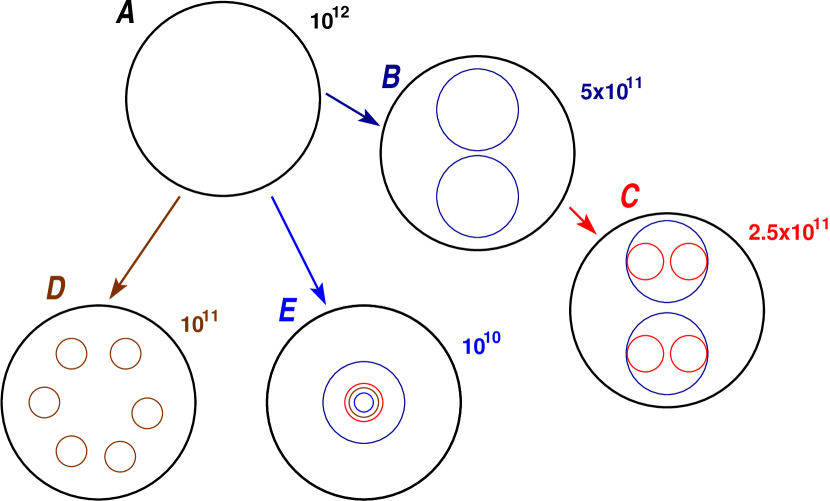
Figure 1.— Model configurations. Schematic representation of our five models and their corresponding constraints. The top right labels indicate the mass of the constraint. The color of the labels indicate the constraint level within each circle.

The common approach to study the evolution of single halos with high numerical resolution and from a cosmological point of view consists of two steps. First, halos of interest are identified in a large cosmological $N$-body simulation. Second, the particles which make up these halos are traced back to the initial conditions. The region enclosing these particles is then re-simulated with a higher resolution. An alternative approach is to find a way of producing the requested structures in agreement with the cosmological model imposed. This can be done by setting up the initial density fields by CRs of Gaussian random fields, following the prescription of Hoffman & Ribak (1991).

The use of CRs to set up the initial conditions as an input for the cosmological simulations has been applied to study several aspects of a structure formation. The CRs are also instrumental in using the data to set up the cosmological simulations. This has been done for studies related to the matter distribution in the nearby universe (e.g.,, Bistolas & Hoffman, 1998; Kravtsov et al., 2002; Romano-Díaz, 2004). However, none of these studies have focused on the evolution of single galactic halos. Below we describe the main characteristics of our CRs, while a mathematical description of the CR formalism is exposed in Appendix A.

2.0.1 The models

We have designed a set of five different models, i.e.,  experiments, to probe different merging histories of a few times $10^{12}h^{-1}M_{\odot}$ halo in an OCDM cosmology. The halo is constrained to have various substructure on different mass scales and locations, designed to collapse at different times. The spherical top-hat model is used here to set the numerical value of the constraints. The model provides the collapse time of the substructures as a function of the initial density. This is used only as a general and rough guide because the substructures are neither spherical nor isolated and hence their collapsing time might vary. Furthermore, the constraints used here do not control the experiments fully. The nonlinear dynamics can, in principle, affect the evolution in a way not fully anticipated from the initial conditions. Even more important is the role of the random component in the CRs. Thus depending on the nature of the constraints and the power spectrum assumed, the random component can form other significant substructures at different locations and mass scales. This can be handled by adding more constraints and varying their numerical values. The price to pay is that the modeled entity will be more “synthetic.”

Model	Constraints ($h^{-1}M_{\odot}$)					$z_{\rm coll}$
	$10^{12}$	$5\times 10^{11}$	$2.5\times 10^{11}$	$10^{11}$	$10^{10}$
A	1					2.1
B	1	2				3.7
C	1	2	4			5.7
D	1			6		7.0
E	1	1	1	1	1	8.9

Note. — Characteristics of the CR models: the first column indicates the model labels. The second, third — sixth columns indicate the level of the mass constraints expressed in $h^{-1}\mathrm{Mpc}$. The given numbers represent the number of constraints imposed at each level for each model. The last column indicates the collapse redshift ($z_{\rm coll}$) of the smallest (in mass) constraint imposed on each model.

Table 2.0.1 presents the main characteristics of our five models. The first column indicates the label of the model. The second-to-sixth columns show the masses of the different constraints (expressed in $h^{-1}M_{\odot}$). The last column states the collapse redshift of the last/smallest constraint in each configuration. All five models are embedded in a region corresponding to a mass of $\sim 10^{13}h^{-1}M_{\odot}$ in which the over-density is constrained to be zero — a region of an unperturbed Friedmann universe. This spatial scale is larger by about a factor of three (in mass) than the size of the computational sphere. Therefore, this constraint cannot be exactly fulfilled, yet it constrains the large scale modes of the realizations to obey it. Model A — our benchmark model, is based only on one constraint of $10^{12}h^{-1}M_{\odot}$. All other models have substructures imposed onto this constraint as illustrated in Figure 1. Each imposed constraint level is indicated by a different color and by its mass at the top right part of model. The position of the constraints is schematic and only serves to get a visual impression of the models. The small-scale constraints imposed over our benchmark model are aimed to modify the merging history of the benchmark model. They change the collapse time as well as the number of major mergers that each model will pass through. In the hypothetical case, when the random part of the CR method does not contribute to the major merger history of the models, model B will experience only one major merger, while model C will have two, and model D can have more than three major mergers. Model E is aimed to mimic a radial collapse by imposing concentric (nested) constraints.

All models have been constructed with the same random seed. This guarantees that the linear external matter distribution and the random component will be the same for all models (Hoffman & Ribak, 1991; van de Weygaert & Bertschinger, 1996). All the density constraints constitute $(2.5-3.5)\sigma$ perturbations, where $\sigma^{2}$ is the variance of the appropriately smoothed field. The constraints were imposed on a box size of $4~{}h^{-1}\mathrm{Mpc}$. In order to avoid the edge effects with the smoothing procedure, the constrained box has been immersed in a $8~{}h^{-1}\mathrm{Mpc}$ box on a cubic grid with 256 grid cells per dimension. The constrained inner box was carved out and resulted in a box size of $4~{}h^{-1}\mathrm{Mpc}$ and 128 grid cells per dimension.

2.1. N-body simulations

Once the constrained initial conditions have been generated, we have applied the Zel’dovich formalism (Zel’dovich, 1970) in order to obtain the initial positions and velocity displacements at redshift $z=120$, using physical rather than comoving coordinates. A sphere of $2~{}h^{-1}\mathrm{Mpc}$ (comoving) radius was carved out from the Zel’dovich evolved fields. All our constraints are totally embedded within this maximum radius sphere. The total number of particles selected within this volume is $\sim 1.3\times 10^{6}$, resulting in a mass resolution of $3.6\times 10^{6}M_{\odot}$. The gravitational softening is 500 pc.

We have evolved each linear density field into the non-linear regime, until $z=0$ (present time), using the updated FTM-4.4 version of our hybrid code (Heller & Shlosman, 1994; Heller, 1995) with the falcON routine (Dehnen, 2002). The code is about ten times faster than the optimally coded Barnes & Hut (1986) tree code. The equations of motion in the FTM-4.4 include the term describing the expansion of the universe. The code has been successfully tested against the Santa Barbara Cluster model (Frenk et al., 1999) (see Appendix B).

Because we are interested in following the merging history of our models as close as possible, we have sampled the dynamical evolution of the systems with 165 time outputs spaced linearly with the expansion parameter $a$. Each halo is resolved at $z=0$ with around $1.1\times 10^{6}$ particles within the virial radius.

3. Mass Accretion Histories

Halos grow according to a hierarchical formation scenario, in which they are assembled via merging of different mass and size halos, together with a more gentle accretion. Several studies have found that the mass accretion history of halos (MAH) may affect the various halo parameters, including $R_{\rm s}$, while maintaining their NFW density profiles (Navarro et al., 1997; Bullock et al., 2001b; Zhao et al., 2003; Tasitsiomi et al., 2004, W02). Therefore, it is important to analyze the MAHs of our five models.

W02 proposed to fit the MAHs of halos by an exponential function in the form:

$$M(a)=M_{0}~{}e^{-\alpha(1/a-1)}$$ (2)

where $a$ is the expansion factor and $M_{0}$ is the final virial halo mass. van den Bosch (2002) arrived to a very similar expression with a two-parameter function using the extended Press-Schechter formalism. Tasitsiomi et al. (2004) found that in many cases Eq. 2 represents a poor fit to the individual MAHs halos, in particular when halos experience an intense and violent activity, up to the present time. Tasitsiomi et al. proposed a more general MAH fit of the form:

$$M(a)=a^{p}~{}M_{0}~{}e^{-\alpha(1/a-1)}$$ (3)

where $p=0$ reduces to the W02 model. Despite the improvement, such a smooth fitting function cannot reproduce all the features in the halo evolution, especially the major mergers.

3.1. Halo identification

Groups and subgroups identification is not a trivial task. Several methods have been proposed which use different “bounding” criteria, e.g., Friends of Friends (Davis et al., 1985), DENMAX (Gelb & Bertschinger, 1994), HOP (Eisenstein & Hut, 1998), SUBFIND (Springel et al., 2001), etc. Different methods are used in order to isolate the halos and subhalos within the halos. We are interested in following the evolution of the main halo through the major branch along its merging tree (see §  4.2). For these purposes we use the publically available code HOP (Eisenstein & Hut, 1998) which computes groups based on the isodensity criteria. Next, we identify the halo centers with the densest particle within the particular halo. Once the centers are found, we grow the halos by adding thin spherical shells and computing the total density until it reaches the value of $\Delta_{\rm c}$ times the mean density of the universe. Therefore, a halo within the virial radius will be specified as a function of redshift as:

$$M_{\rm vir}(z)=\frac{4\pi}{3}\Delta_{\rm c}(z)\ \rho_{\rm b}(z)\ R_{\rm vir}(z)\,,$$ (4)

where $\Delta_{\rm c}$ is the critical density and it is computed using the top-hat model, $\rho_{\rm b}$ is the universe density and $R_{\rm vir}$ is the virial radius of the halo.

4. Results

4.1. Model evolution

A halo of $\sim 10^{12}M_{\odot}$ has formed by $z=0$ in all of our models, except in model B. At the present time, this model harbors two halos of $\sim 5\times 10^{11}M_{\odot}$ which are on their way to merge. The final collapse time (i.e., the time of the last major merger) of the halos is as follows: B, E, A, D and C, from the earliest to the latest. Defining the halo formation as the time when half of the mass is in place, results in the same order as above. In comparison, the top-hat model predicts a different order of collapse times. This is expected because the random component of the CR method can introduce other structures of the same level as the constraints. As a result, the merging history and the collapse time imposed by these constraints will be modified (Section 2.0.1; see also van de Weygaert & Bertschinger, 1996). Since we have warranted that our five models have the same random component, all of them will be affected in the same way.

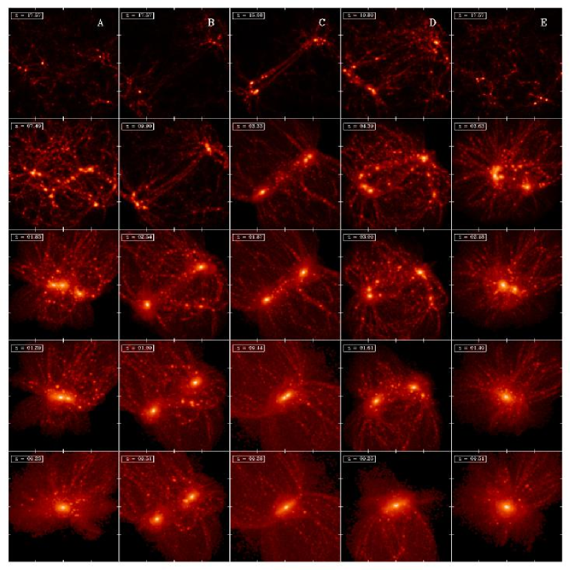
Figure 2.— Time evolution snapshots for the five models. Models are arranged from left to right columns: A, B, C, D and E. Each frame represents the logarithmic density field weighted by the mean density at the given time. The top left labels in each frame indicate the redshift of a given snapshot.

The evolution of the models can be observed in their density projections (Fig. 2) and the respective merging trees (Fig. 3). The effect of different constraints imposed on the halos can be noticed from their evolution on these diagrams. Figure 3 is a schematic representation of the halo growth and the merging history of the models. The size of the circles is proportional to the mass (left column numbers) of the depicted halos (see Section 4.2). This representation underscores the effect of the CRs on the evolution of these models. The model A evolves through three major mergers. Since model B harbors two very similar halos, we only present the evolution of one of them (the most massive). It has two nearly simultaneous major mergers of an exceptional strength, in its early phase. Because the halo is out of the dynamical equilibrium during this time, we consider this double merger event as a single one. Model C frame shows the evolution of the four constraints, their collapse into two major entities and formation of one single halo. In the model D, the six constraints and their development into two major halos and the final collapse can be clearly followed from the respective tree. The early formation of the model E through two recognizable major mergers is neatly shown in its merger tree panel.

Figure 2 exhibits density maps in the co-moving coordinates of the models for five different epochs taken from the respective merger trees. The first column refers to model A, the second — to B, the third — to C, the fourth — to D, and the last one — to model E. The color scale is proportional to the logarithm of the density field. The first row shows the different initial conditions between the five models. The last row shows the final state of the halo. Shown are the random frames after the last major merger that each model experienced, and not the last snapshot of our simulations. The intermediate frames illustrate different dynamical epochs for the halos. In model A, the frames depict the moments prior to two major mergers. Model B frames clearly show the two imposed constraints — the system, although gravitationally bound, does not merge at the present time, but it will do this in the future. Models C and D show the early collapse of the small constraints, the formation of the two major clumps and their way to collapse into a single halo. Model E (the first model to collapse into a $\sim 10^{12}M_{\odot}$ halo) shows a more radial filamentary structure around it, a direct consequence of the imposed constraints. The amount of substructure changes from model to model, with the model D exhibiting the richest substructure.

4.2. Merger trees

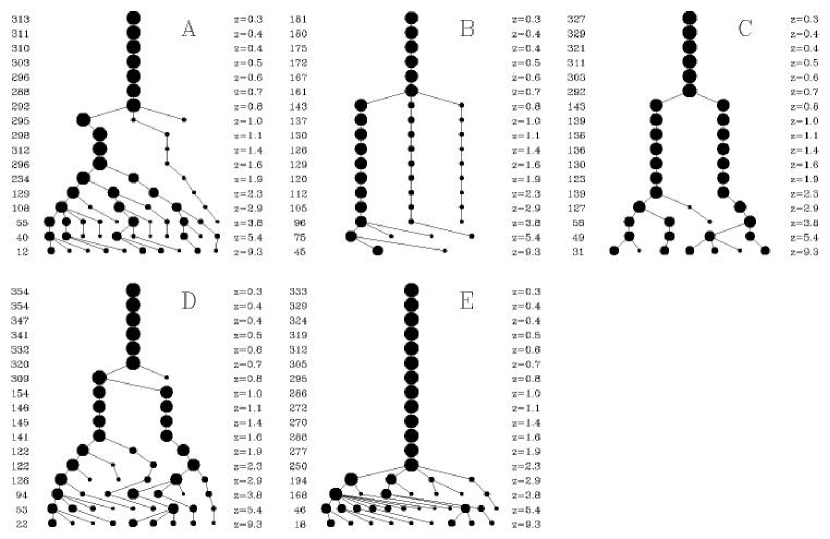
Figure 3.— Schematic merger trees for our five models. The right columns indicate the redshift frame. Circles are proportional to the mass of the halos at the given times.

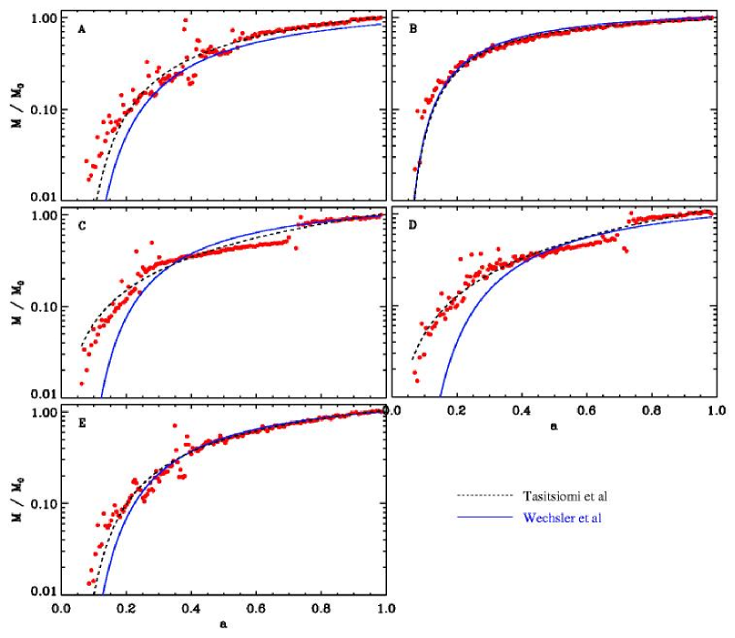
Figure 4.— Mass Accretion Histories for our five models. The red dots indicate the measured mass normalized by the final mass of the respective halo. The blue continuous line represents the best fit from the W02 model, while the dashed black lines the Tasitsiomi et al. (2004) model.

Since we have identified all halos for basically each of the output times of our simulations (we have found halos for all models from $z\approx 20$ onwards), we can construct detailed merger trees along the path of the main progenitor. Using the main halo at a given time, we trace back the identified particles to the previous time step and correlate them with the most massive halos at this time. The progenitor is identified with that halo which contains at least $50\%$ of the particles of the parent halo. We also follow the trajectories of their respective centers. This will assure that we follow the right predecessor. Once a branch has been chosen along the halo’s tree, we follow it up until this branch opens again and repeat the same procedure. Note that in this way the followed halo is not necessarily the most massive halo at all times in the simulation, but rather most of the time.

Figure 3 shows the merger trees for our five models. The size of the circles is proportional to the logarithm of their respective masses (indicated by the numbers located by the left columns of each panel) at the respective times (indicated by the right columns labels). The degree of accuracy of the trees depends upon the number of identified structures at each time step. In general, our merger trees consider all identified structures per time step, but for the sake of clarity we have only plotted the relevant halos to illustrate the evolution of the models.

Once the merger trees have been elaborated, one can construct the MAHs straightforward. The red dots in Figure 4 represent the measured masses normalized with respect to their respective final halo masses. The blue solid lines represent the best fit according to the W02 model, while the dashed black lines — to the Tasitsiomi et al. (2004) model. The fits were obtained by $\chi^{2}$ minimization. In general, the Tasitsiomi et al. model represents a better fit to all models than the W02 one. However, both methods fail in reproducing the early parts of the MAHs. The deficiencies of the W02 model are emphasized in models C and D which have a more violent history than the rest of the models. On the other hand, the Tasitsiomi et al. fits do not represent the full MAH of such halos, see for example the large deviations at $a\sim 0.6$ for both models (the time between two major mergers). It is clear that neither fits reproduces the MAH of a halo throughout its entire history. At best such fits can accurately describe the MAH within one single passive evolution phase. Having stated that, we have used Model B, which has the longest quiescent phase, to test the quality of the analytical fits.

4.3. NFW analysis

For all halo models, we fit the NFW profiles as a function of time and thus follow the cosmological evolution of their parameters ($R_{\rm s}$ and $\rho_{\rm s}$). Many factors may affect the fits of analytical profiles to the observed (simulated) ones: the choice of binning, the merit function, the weights assigned to the data points, the range of radii used in the fitting (Tasitsiomi et al., 2004). We have divided each halo into spherical shells equally spaced logarithmically until $0.6R_{\rm vir}$, in order to give more statistical weight to the inner regions of the halos. We have chosen this radius since fitted profiles do not change substantially beyond this radius. In case that a massive subhalo is nearby (we define such halos as those with mass $>0.3M_{\rm vir}$) the density profiles are non-monotonic and bumps at the data point distributions are present. We avoid such bumps by performing fits until $min(0.6R_{\rm vir},0.5d_{\rm h})$, where $d_{\rm h}$ is the distance to the given subhalo. We have set the minimum fitting radius equal to $2\epsilon$ (where $\epsilon$ is the gravitational softening imposed in the $N$-body force calculation) in order to avoid two-body interactions. This minimum radius is well within the range where a density profile for the characteristic of our models can be considered to be “resolved” (e.g., Binney, 2004; Diemand et al., 2004; Reed et al., 2005a). The fitting procedure is performed by weighted $\chi^{2}$, where the residual in a given shell is normalized by its own density.

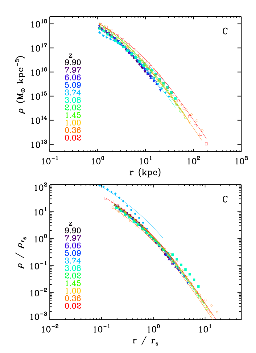
Figure 5.— NFW fits for model C. The symbols are the data measurements (symbols and colors indicate different halo epochs), while the continuous lines represent the best NFW fit. The upper panel shows the normal fits, while the bottom panel presents the normalized fits and data.

The upper panel of Figure 5 shows the NFW fits for 12 different time outputs (indicated by different colors and symbols) of model C. The bottom panel presents the same fits but normalized by $R_{\rm s}$ and $\rho_{\rm s}$ respectively. Symbols indicate the data measurements while the continuous lines the best fitted models. Most of the fits are in good agreement with the measured data. Such fits correspond to the steady/quiet epochs in the halo evolution. The fits that do not follow the observed data correspond to those epochs where the halo is passing through a violent episode (major merger).

4.4. Virial quantities

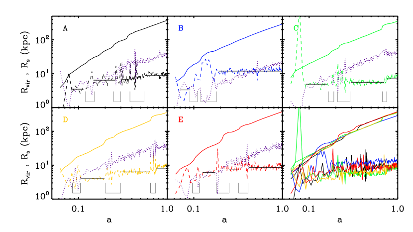
Figure 6.— Evolution of the virial radii $R_{\rm vir}$ (solid lines), characteristic radii $R_{\rm s}$ (dashed lines) and concentration parameter $c$ (dotted lines). Each panel refers to a different model. The bottom right-most panel compares directly the $R_{\rm vir}$ and $R_{\rm s}$ quantities.

By following the evolution of the halo virial quantities ($R_{\rm vir}$, $M_{\rm vir}$), we are able to distinguish, as a function of time, the main large scale characteristics between the different models. Figure 6 shows the evolution of the virial radii for the different models (solid lines). In the bottom right-most panel, all profiles have been superimposed for a better comparison. Note that the virial radius grows almost linearly with $a$ during the quiescent phases in all models. The sudden increases correspond to the epochs where violent activity takes place indicated by the square brackets at the bottom of each panel. The width of the brackets shows the duration of the violent event. Despite the fact that the various models have different violent epochs at different times, all of them (apart from model B) seem to converge to the same virial values once their last major merger has taken place. This happens since the larger constraint has been set to form a $\sim 10^{12}M_{\odot}$ halo. The violent activity is more noticeable in the virial mass (Figure 7, continuous lines) where the large jumps indicate a substantial mass component addition to the main progenitor. During the quiescent epochs, mass is only deposited very slowly through accretion and minor mergers that are being tidally disrupted outside $R_{\rm s}$. This can be observed as a very gentle increase in the mass trajectories between the major mergers.

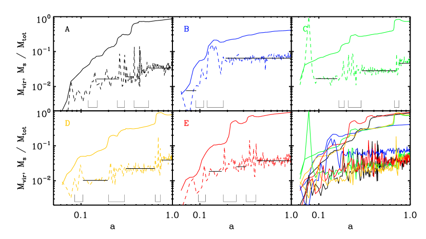
Figure 7.— Evolution of the virial mass $M_{\rm vir}$ and the characteristic mass $M_{\rm s}$ (in units of the total mass, $M_{\rm tot}$) for all models. The bottom right-most panel presents all mass trajectories. Different colors correspond to different models.

4.5. Inner characteristic quantities: $R_{\rm s}$, $M_{\rm s}$, $c$, etc.

Figure 6 also exhibits the evolution of the inner radius $R_{\rm s}$ (broken lines), and the concentration parameter $c$ (dotted lines). Subject to a $\sim 10\%$ jitter, $R_{\rm s}$ is a growing step function. In other words, $R_{\rm s}$ grows only at the moments when major events take place (indicated by the bottom square brackets) and it remains constant along the quiescent phases. The horizontal lines which overlie the distributions are the average of $R_{\rm s}$ between the major events. Note that the $R_{\rm s}$ distributions follow closely the mean lines for the whole ranges. The amplitudes of the jumps are proportional to the degree of “violence” of the encounters, in other words, to the change in the kinetic energy that the system experiences (Paper I and Sec. 4.6). The large jumps and discontinuities in $R_{\rm s}$ are a clear indication of major mergers taking place. In the bottom right-most panel, all $R_{\rm s}$ trajectories can be compared more closely. All models reach approximately the same value after their last major merger (apart from model B), independently of the number of major mergers and the epoch they took place. It is interesting to see that model B has the largest $R_{\rm s}$ among all the models.

The corresponding concentration parameters $c$ (Figure 8) display an erratic behavior at early epochs, e.g., $a\sim 0.1$. However, starting with $a\sim 0.2$, the trajectories become more coherent. Different model $R_{\rm s}$ and $R_{\rm vir}$ exhibit the tendency to converge after their last major merger, while $c$ does not (the bottom right panel of Fig. 8). The jitter present in $c$ is mainly dictated by the $R_{\rm s}$ behavior. It has been claimed that $c$ grows linearly with time (W02). However, since we resolve the step-like evolution of $R_{\rm s}$ and the discontinuities in $R_{\rm vir}$, $c$ appears to grow linearly only during the quiescent phases. We show this clearly in Fig. 8, where the black continuous lines represent the best linear fits for the given quiescent phases. The numbers shown within each frame represent the best fit parameters for the slopes, $m$, and zero-points, $s$. Note that the slopes decrease after each major event. The intermediate slopes for Models A and E are unreliable and were not fitted because the halos do not have enough time to relax between these major events.

Model B has been assembled earlier compared to other models, but it possesses the smallest $c$ at the present time. This behavior appears to be in contrast with the previously reported results (i.e. Bullock et al., 2001b, W02) which claimed that the halos assembled early, when the universe has a larger density, are more concentrated and have a larger $c$ parameter. However, $R_{\rm s}$ and, therefore, $c$ are related not only to the density of the universe at that time, but also to the intensity of an event during the formation epoch of this particular halo (Fig. 8, see also Paper I). Since model B has experienced the strongest event in terms of the deposited kinetic energy $K_{\rm s}$ within $R_{\rm s}$ (see Fig. 11), it has the larger $R_{\rm s}$ and, therefore, the smallest $c$.

It is interesting that both models C and D seem to depart from the general trend observed by the rest of the models at $a\sim 0.7$. This corresponds to the epoch in which both models went through their last major merger. After these events took place, the $c$ trajectories lower their amplitude and join the general trend. The growth of $c$ seems to be nearly linear with respect to $a$  during the quiescent phase, indicating that its behavior is dominated mainly by $R_{\rm vir}$ (see also Fig. 6).

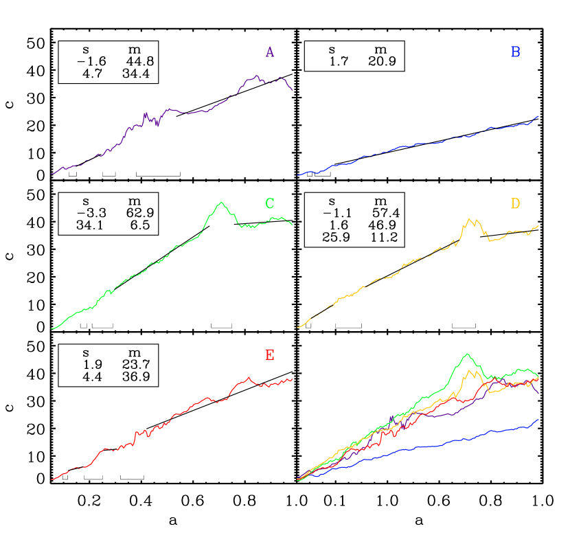
Figure 8.— Linear plot of the evolution of the concentration parameter, $c$, for the five models. The individual curves has been smoothed over ten points. The continuous lines represent the best linear fits for various quiescent phases. The fitting has been avoided for short phases because of the associated errors. The enclosed top-left parameters indicate the best zero-points, $s$, and slopes, $m$.

The mass $M_{\rm s}$ is computed by counting particles within this radius and hence it is a top-hat mass. The $M_{\rm s}$ behavior is presented in Figure 7 (dashed lines) for all five models, and is very similar to that of $R_{\rm s}$— it remains constant during the quiet phases and grows only during the violent events. The horizontal lines indicate (as in the case of $R_{\rm s}$) the mean $M_{\rm s}$ within the given time intervals. Similarly to Fig. 6, the bottom brackets in each frame indicate the time and duration of the major mergers. The model B also has the largest $M_{\rm s}$, as noted at the bottom right-most panel where all $M_{\rm s}$ trajectories are depicted. At the time of the violent events associated with the core growth, the system is not in a virial equilibrium and so the density profile is undefined causing the erratic appearance of spikes in $R_{\rm s}$ and $M_{\rm s}$ (e.g., Figs. 6, 7 and  9).

4.5.1 General trends in $R_{\rm s}$

The $R_{\rm s}$ behavior detected in Paper I and in the previous section has been only addressed from the ‘typical’ NFW fitting procedures. As has been pointed out in Section 1, there is a controversy whether the inner slope is $-1$, steeper or shallower, or it is not universal at all. This raises the question whether the $R_{\rm s}$ behavior is driven by the change in the inner slope (a mere effect of the NFW fitting procedure) or by a real change in $R_{\rm s}$. To answer this question, we fit the halos using three alternative density profiles, i.e., by applying the generalized law (Zhao, 1996):

$$\rho(r)=\frac{4\ \rho_{\rm s}}{(r/R_{\rm s})^{\gamma}(1+(r/R_{\rm s})^{\alpha})^{\frac{\beta-\gamma}{\alpha}}}\,,$$ (5)

where $(\alpha,\beta,\gamma)=(1,3,1)$ for a NFW, $(1.5,3,1.5)$ for a Moore et al. (1999), $(1,3,1.5)$ for a Jing & Suto (2002) and $(\alpha,3,\gamma)$ for a more general density profile. In general, the fitting procedure varying the parameters $\alpha,\beta$ and $\gamma$ leads to degeneracies between the parameters (see Klypin et al., 2001; Tasitsiomi et al., 2004). With this approach, it is possible to find “excellent” fits using parameter values far from what have been found for that kind of halos. Therefore, in order to get physically meaningful fit estimates one has to constraint the parameter range.

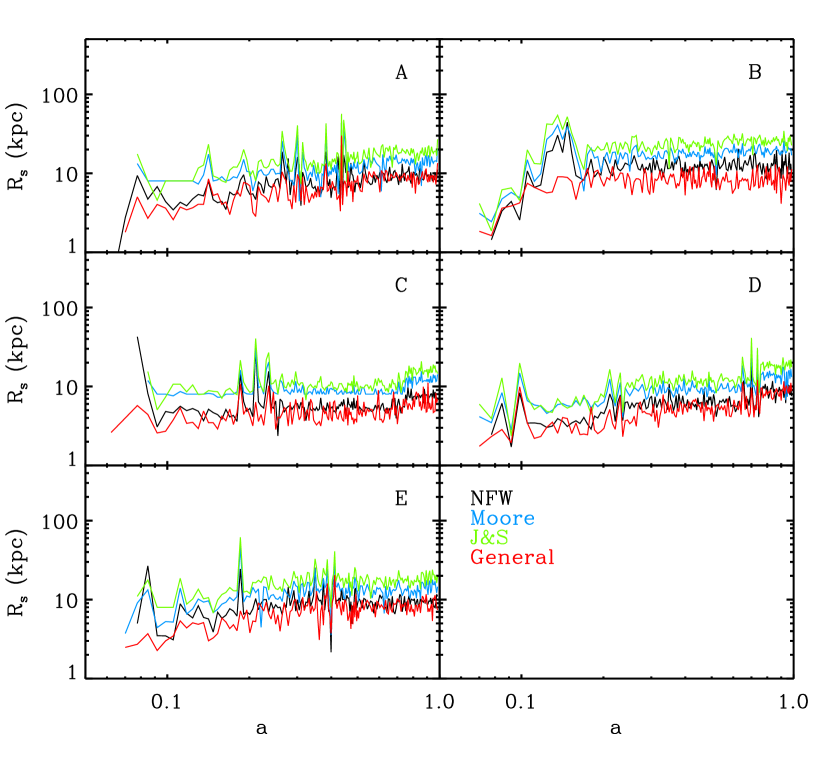
Figure 9.— Evolution of density profiles using various fits to our five models. The black lines represent the NFW profiles, the blue lines — the Moore et al. profile, the green lines — the Jing & Suto profile, while the red lines — the general profile of Zhao.

Figure 9 shows the evolution of $R_{\rm s}$’s obtained from four different fitting profiles indicated by different colors. Note that all profiles show the same behavior, $R_{\rm s}$ remains constant during the quiet phases and increases abruptly during the violent epochs. It is expected that the application of different density profiles will result in differing values of $R_{\rm s}$, which can be correlated (e.g., Tasitsiomi et al., 2004). The general fits (red lines) are very close to the NFW fit (black lines). This effect could be due to our use of NFW values to constrain the general fitting.

Reed et al. (2005a) found that the inner slope does not decrease in time, but rather stays constant during the quiescent phase, by applying a semi-general fitting to the halo evolution. We can apply this observation to each of the phases and conclude that the slope also changes only during the violent events. Combining these two effects, one expects that the NFW $R_{\rm s}$ displays a similar behavior to $R_{\rm s}$ obtained from other fitting procedures; Fig. 9 shows clearly this point. Because we observe that $R_{\rm s}$ grows as a step function even for the general fit, this indicates that not only a change in the inner slope is involved, but rather a real behavior/change in $R_{\rm s}$.

4.5.2 The characteristic density $\rho_{\rm s}$

The characteristic density has the opposite behavior to $R_{\rm s}$ — it is a decreasing function of time, so their product, $\rho_{\rm s}$$R_{\rm s}$, appears nearly constant with time for all models and across the violent and quiescent phases. As $R_{\rm s}$ also $\rho_{\rm s}$ is affected by the $10\%$ jitter. At major mergers it drops considerably and fluctuates until it reaches a plateau where it remains constant. At the next major merger it drops and reaches a new, lower level plateau.

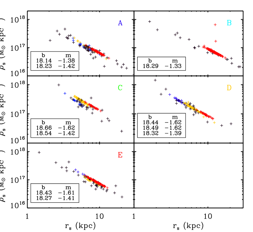
Figure 10.— The characteristic density $\rho_{\rm s}$ as a function of the characteristic radius $R_{\rm s}$. The colors indicate the different quiescent phases that each halo passes through. The individual slopes, $m$, and the zero points, $s$, are specified for separate quiescent phases for every model (see text for further details). The fitting has been avoided for short phases because of associated errors.

We have investigated the possibility of a correlation between $R_{\rm s}$ and $\rho_{\rm s}$within the jitter of the quiescent phases. Naively one expects that $R_{\rm s}$ and $\rho_{\rm s}$ in the jitter will produce a scatter diagram. However, Figure 10 shows that a strong correlation exists between both quantities: larger $R_{\rm s}$ correspond to smaller $\rho_{\rm s}$. Moreover, a one-to-one correlation exists between $R_{\rm s}$ and $\rho_{\rm s}$ across the full range of $R_{\rm s}$. The different colors represent the various quiescent episodes that the halos experience through their MAHs. The black symbols correspond to the violent episodes and to the early assembly time of the halo. The scattered points located above and below the main trends mark the violent events. Model B displays a single phase since this halo formed at an early phase and remained quiescent for most of its evolution. Models C and D, which display three well identified quiescent phases, have three well defined point distributions separated from each other. Models A and E present very similar distributions. We have performed linear fits to the logarithmic distributions for all models of the form

$${\rm log}~{}\rho_{\rm s}=m\ {\rm log}~{}R_{\rm s}+b\,.$$ (6)

in two fashions. First, by including all plotted points; second, by separating the quiescent phases and fitting each. The upper legends at each panel indicate the slope of the individual fits $(m)$ and their zero points $(b)$. Note that all the zero points lie about log $\rho_{\rm s}$$\sim 18.2$. The slope averaged over all models is $m=-1.37\pm 0.03$. Even the slope constructed from different epochs (given by different colors in Fig. 10) shows very little scatter around the average value. This value appears to be independent of particular halos and of their evolution. Furthermore, the points corresponding to the later time (i.e., red color) are consistently located in the tail of their respective distributions. This color order is a direct consequence of $R_{\rm s}$ and $\rho_{\rm s}$ monotonic evolution discussed earlier. The measured jitter ($10\%$ or so) in both $R_{\rm s}$ and $\rho_{\rm s}$ can be recognized now as the individual trends (colors) for each model. This implies that a clear order exists in the halo variations. Specifically, we find that $\rho_{\rm s}$$\sim$$R_{\rm s}$^-1.59±0.15 during the jitter at early quiescent, i.e., $a<0.5$, epochs in all models, while $\rho_{\rm s}$$\sim$$R_{\rm s}$^-1.39±0.04 for later times. When translated to $M_{\rm s}$—$R_{\rm s}$ correlation, this amounts to $M_{\rm s}$$\sim$$R_{\rm s}$^1.41 and $M_{\rm s}$$\sim$$R_{\rm s}$^1.61, respectively. The simplest interpretation of these correlations is that they are driven by density fluctuations which originate at radii between the cusp (i.e., slope = –1) and $R_{\rm s}$ (i.e., slope = -2).

Lastly, the shifts between different colors in Fig. 10 come from violent events which deposit kinetic energy and mass within $R_{\rm s}$ and separate the quiescent evolution (see section 5.5). Our results are in agreement with those reported by Zhao et al. (2003), who found that $M_{\rm s}$$\sim$$R_{\rm s}$^1.44 holds in the “slow accretion phase” (gentle accretion), and $M_{\rm s}$$\sim$$R_{\rm s}$^1.92 in the “rapid accretion phase.” The difference results from our ability to separate the violent and quiescent phases — we have excluded the black symbols in Fig. 10 from the fitting, because they correspond either to the very early assembly or later violent times. This reduces the scatter in our fits below that of Zhao et al.

4.6. Kinetic and Potential energy and the virial ratio

We have computed the internal kinetic energy $K$ of the main halo along its merger tree. For each time output, we have computed the kinetic energy, $K_{\rm r}=\sum_{i=1}^{n_{\rm r}}\frac{1}{2}m_{\rm i}\sigma_{\rm i}^{2}$, where the summation goes for all objects enclosed within a radius $r$, $n_{\rm r}$, and $\sigma_{\rm i}$ represents the velocity dispersion of a given object $i$ of mass $m_{\rm i}$.

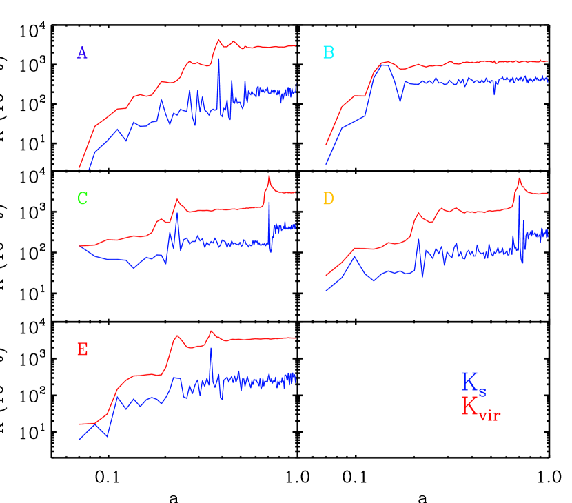
Figure 11.— Kinetic energy for all models as a function of time. The blue distributions represent the characteristic kinetic energy, while the red ones the virial distributions. Labels are the same as in the previous figures.

Figure 11 shows the evolution of the internal kinetic energy computed within the radii $R_{\rm s}$ (blue lines) and $R_{\rm vir}$ (red lines). As in the case of $R_{\rm s}$, $K_{\rm s}$ also increases as a step function, i.e.,  only at the major events and it remains constant during the quiescent phases. On the other hand, $K_{\rm vir}$ grows in two different ways, it grows suddenly at the violent phases as $K_{\rm s}$ does, while during the quiescent phases it grows in a very gentle way.

From Fig. 11, one can realize that $K_{\rm s}$ of model B has the largest value of all models while its $K_{\rm vir}$ is the smallest from all models. This is a mere reflection of their mass accretion histories. Furthermore, the growth of model B energy curve is the most abrupt of all models, occurring at an early redshift ($z\sim 9$). This halo went through a very violent and rapid formation epoch at this early $z$. This violent formation event resulted in the largest $R_{\rm s}$ in our sample, although it is the less massive of the five models.

The potential well of the halos is also constructed from their respective MAHs. Zhao et al. (2003) found in their simulations that the potential well is mainly build up in the so-called fast accretion phase, while remaining almost constant during the slow accretion phase. Figure 12 shows the evolution of the potential energy ($\phi$) for our set of models. This $\phi$ is computed by including all particles within a given radius, namely $R_{\rm s}$ and $R_{\rm vir}$. Since there is no mass accretion within $R_{\rm s}$ in the quiescent phases, it is expected, therefore, that the potential $\phi_{\rm s}$ remains constant during such phases and only deepens at the major events when mass is accreted within $R_{\rm s}$. In the case of the potential within $R_{\rm vir}$, where the halo growth is due to violent and gentle mass accretion, $\phi_{\rm vir}$ uncovers these two phases as well. It sinks substantially at the major events and it deepens in a very gentle way during the quiescent phases. This general behavior indicates that the potential wells are only formed and substantially modified at the violent events. The main difference with the Zhao et al. (2003) analysis is that they only recognize a single early fast accretion period, while in our models the later quiescent phase is intermitted by the violent events.

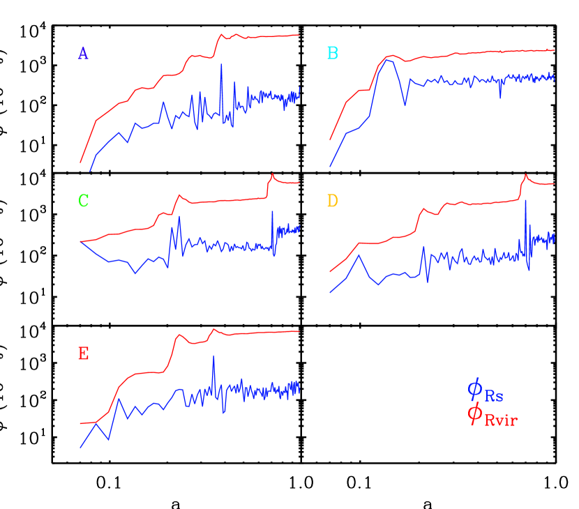
Figure 12.— Potential energy for all models as a function of time. Labels and colors are the same as in previous figures.

The way energy is acquired by the halos and the details of the formation of the respective potential wells reinforces our view of the halo growth process. Energy is deposited into the halo via gentle and violent mass accretion. The latter affects the whole halo since both $R_{\rm s}$ and $R_{\rm vir}$ grow during such events, while the former affects only the exterior part of the halo. Gentle accretion and minor mergers deposit their mass and energy within this outer region. Energetic events such as those produced by the major mergers are able to reach the halo core, since they are more strongly gravitationally bound. Part of their mass and energy are deposited inside the halo core.

The interplay between the kinetic and potential energies within a given halo can be better understood in terms of the virial ratio defined as $Q_{\rm r}=-2K_{\rm r}/\phi_{\rm r}$, where the subindex $r$ denotes the radius at which this quantity is computed. At the virial radius, $Q_{\rm r}$ should be close to unity for systems in virial equilibrium and nearly isolated. Because virialized structures are bordered by infalling and outgoing material, the convergence of $Q_{\rm r}$ to unity at $R_{\rm vir}$ should not be fully expected (see e.g., Macciò et al., 2003; Shaw et al., 2005). However, since our models are basically constructed in isolation, after their respective last major merger, $Q_{\rm vir}$$\rightarrow 1$. Indeed, this can be observed in Figure 13 where the solid lines represent the $Q_{\rm vir}$ quantities for each model. The pronounced spikes along each track represent the time of the major events and the considerable departure from the virial equilibrium. On the contrary, $Q_{\rm s}$ is not expected to be close to unity, since this region experiences “pressure” from overlying halo. Note that during the quiescent phases $Q_{\rm s}$ remains constant and, as in the case of $R_{\rm s}$, jumps to another stationary trajectory when the major events take place.

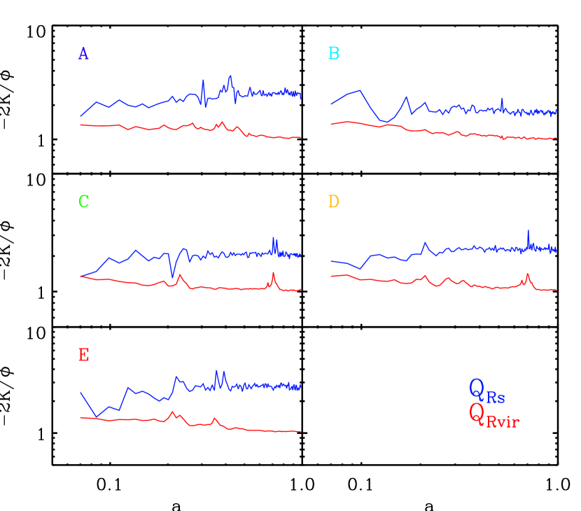
Figure 13.— Virial ratios for all models as a function of time. Labels and colors are the same as in previous figures.

4.7. Shapes

We have analyzed the shapes of our halos as a function of time by using the inertia tensor, for $R_{\rm s}$ and $R_{\rm vir}$ respectively, using the unweighted moment of inertia defined as $I_{\rm ij}=\sum_{n=1}^{n_{\rm r}}x_{\rm i,n}x_{\rm j,n}$, where $x_{\rm i},x_{\rm j}$ represent the $i,j$ Cartesian components of the position of a particle $n$ and the summation extends over all particles enclosed within the given radius $r$ ($=$ $R_{\rm s}$, $R_{\rm vir}$). Allgood et al. (2006) showed that the weighted and unweighted moments of inertia used to compute halo shapes differ only by $10\%$. Our aim here is to compute the halo shape evolution at various radii as a function of their merging history. Therefore, we divide the halos into spherical shells. An alternative approach is to compute the shapes within isosurfaces of density or potential (Berentzen & Shlosman, 2006). Since so far we used quantities defined within the $R_{\rm s}$ and $R_{\rm vir}$ spherical distributions, we choose the former approach for consistency.

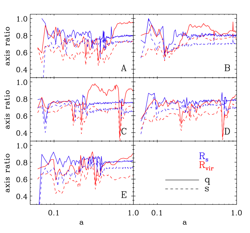
Figure 14.— Axes ratios for our five models. For each model we present $s~{}(\equiv c/a,$ dashed lines) and $q~{}(\equiv b/a,$ solid lines) ratios for $R_{\rm s}$ (blue lines) and $R_{\rm vir}$ (red lines).

We compute the eigenvectors and eigenvalues of the moment of inertia matrix and define the axes of the ellipsoid as $a,b,c={\sqrt{(}\lambda_{\rm a},\lambda_{\rm b},\lambda_{\rm c})}$, where $\lambda_{\rm i}$ corresponds to the $i$th eigenvalue, and they are arranged in the descendent order (i.e.,  $\lambda_{\rm a}>\lambda_{\rm b}>\lambda_{\rm c}$). These axes are normally described in terms of the ratios $s\equiv c/a$, $q\equiv b/a$ and $p\equiv c/b$.

Figure 14 displays the shape evolution of $R_{\rm s}$ and $R_{\rm vir}$ indicated by the red and blue colors respectively. The dashed lines correspond to the $s$ parameter of both radii, while the solid lines — to the $q$ number. Clearly, all models are prolate within $R_{\rm s}$. This result is in agreement with the analysis of Allgood et al. (2006) at small radii, and of Berentzen & Shlosman (2006). Within $R_{\rm s}$ the halo shapes are unperturbed and only change at the major mergers. On the other hand, the $R_{\rm vir}$ shapes change during the quiescent epochs as well, mainly because gentle accretion is not isotropic. The $s$ and $q$ at $R_{\rm vir}$ indicate that there is a tendency for the halos to become less triaxial with time.

4.8. Angular momentum considerations

One of the drawbacks of the present simulations is the lack of the external tidal field presence in our simulations. Although our simulations have accounted for the tidal field within the original box of $8~{}h^{-1}\mathrm{Mpc}$, this volume does not suffice to include the large scale tidal contributions. Nevertheless, this affects only the final phases of the formation of the halo. At earlier times, the main halo is surrounded by other halos of about the same mass that torque it. Therefore, the measured angular momentum will be mainly produced by the direct interactions of the halo with those substructures created with the constrained random field. Any differences between the models will be attributed to their different merging histories.

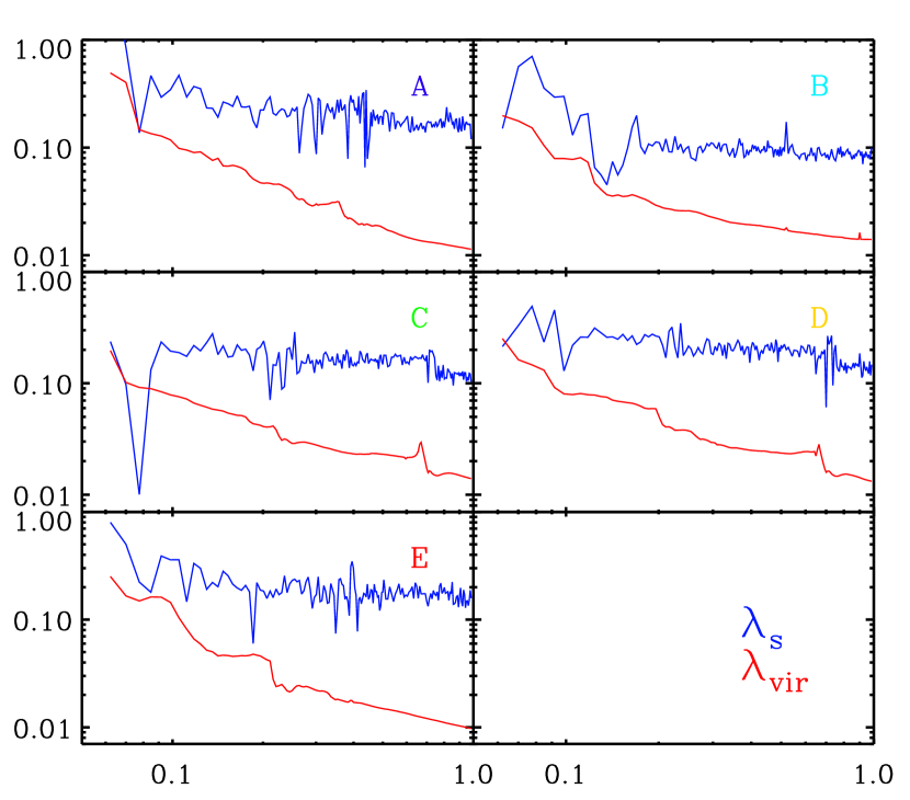
Figure 15.— Spin parameters for our five models computed at $R_{\rm vir}$ and $R_{\rm s}$.

The angular momentum can be expressed in term of the dimensionless spin parameter (e.g., Peebles, 1969) $\lambda\equiv J|E|^{1/2}/(G\,M^{5/2})$, where $J,~{}E$ and $M$ are the total angular momentum, energy and mass of the system, and $G$ is the gravitational constant. The value of the spin parameter roughly corresponds to the ratio of the angular momentum of a halo to that needed for rotational support (see e.g., Padmanabhan, 1993). Typical values of the spin parameter of individual halos from $N$-body simulations are in the range $[0.02,0.11]$ (Barnes & Efstathiou, 1987; Ryden, 1988; Warren et al., 1992; Steinmetz & Bartelmann, 1995; Cole & Lacey, 1996; Gardner, 2001; Bullock et al., 2001a). The spin parameters in $N$-body simulations are independent of the cosmological model (Barnes & Efstathiou, 1987; Warren et al., 1992; Lemson & Kauffmann, 1999; Gardner, 2001), halo environment or halo mass (Lemson & Kauffmann, 1999). The only correlation that has been found is with the time of the last major merger: halos that had a recent major merger have larger spin parameter (Gardner, 2001).

Bullock et al. (2001a) proposed an alternative and more practical way to compute the spin parameter $\lambda^{\prime}\equiv J/(\sqrt{2}\,M\,V\,R)$, where $J$ is the angular momentum within a spherical volume of radius $R$ with mass $M$ and $V$ is the halo circular velocity at radius $R$, $V^{2}=GM/R$. This definition reduces to the standard one when measured at the virial radius of a truncated singular isothermal halo (Bullock et al., 2001a). In $\lambda^{\prime}$ definition, $J$ is defined as ${\bf J}=\sum_{i=1}^{n_{\rm r}}{\bf r}_{\rm i}\times m_{\rm i}{\bf v}_{\rm i}$. We have adopted the Bullock et al. definition, hereafter $\lambda$. Figure 15 shows the evolution of the spin parameter computed at the two usual radii, $R_{\rm vir}$ and $R_{\rm s}$, $\lambda_{\rm s}$ and $\lambda_{\rm vir}$(blue and red lines respectively). The sudden changes in $\lambda_{\rm vir}$ are clearly correlated with the major events involving each halo. $\lambda_{\rm vir}$ exhibits the tendency to decline during the quiescent epochs (see also Vitvitska et al., 2002). This is a consequence of fast increase in $R_{\rm vir}$$\sim a$ during these epochs, which makes the denominator in $\lambda$ to grow faster than $J$ for any reasonable scenarios of the halo growth. Models A and E have the lowest virial spin parameter because most of the accreting material has already joined them. Model B has the largest $\lambda_{\rm vir}$ by the end of the simulations — it has the smallest main halo and a substantial amount of material is locked in its companion and around it.

The behavior of $\lambda_{\rm s}$ differs somewhat from that of $\lambda_{\rm vir}$. It confirms that the halo core grows only via accretion of major mergers and minor mergers do not play a role. Under these conditions, one expects that $\lambda$ will be conserved. The blue lines of Fig. 15 shows precisely this type of behavior. The spin parameter decreases only at the major events and remains constant during the quiescent phases in most of the models which exhibit the same $\lambda_{\rm s}$ value. However, Model B has the lowest $\lambda_{\rm s}$, which is due to a smaller number of major mergers it has experienced.

This analysis shows that although the models miss large scale torques, this does not represent a considerable problem for their evolution. While the models have been constrained to the same initial sizes and masses, no constraint has been imposed on the spin parameter. Because the number of major mergers is the same in all models except the Model B, the final spin parameter differs little between them.

5. Discussion and Conclusions

We have investigated the effect of a different assembly history on the final structure of the DM halos. We have employed the Constrained Realization method of random Gaussian fields in order to create the initial conditions for a $10^{12}h^{-1}M_{\odot}$ halo, which has been evolved subsequently by means of the $N$-body simulations. Five different variants of the same final halo have been simulated and analyzed using a sufficient mass resolution to identify the halos and subhalos at early redshifts ($z>10$), and a sufficient time sampling in order to closely follow their dynamical evolution. The model evolution has been quantified in terms of parameters which characterize the NFW as well as other, non-NFW density distributions.

The evolution of a given halo can be characterized by a number of quiescent phases of a slow evolution intermitted by violent episodes of major mergers. We find that the inner halo is in a state of a dynamical equilibrium during the former phases, and its density is well approximated by an NFW profile. Furthermore, the NFW characteristic radius $R_{\rm s}$ appears to be the best gauge of the dynamical evolution of a halo. It remains constant in the quiescent phases and it grows discontinuously during the violent episodes. Other variables that characterize the inner structure, i.e.,  within $R_{\rm s}$, behave in a similar way in their growth or decline, e.g., $\rho_{\rm s}$, $M_{\rm s}$, $\lambda_{\rm s}$, etc. Between the major mergers, the halos evolve very passively. This means that a gentle accretion does not influence the behavior of the characteristic quantities. The minor mergers only contribute to the gentle growth of the external halo and to a decrease of the spin parameter. We note that the product $\rho_{\rm s}$$R_{\rm s}$ is nearly constant in time showing only a very slight decline. The significance of this will be discussed elsewhere.

On the other hand, the virial parameters, e.g., $R_{\rm vir}$, $M_{\rm vir}$, $\lambda_{\rm vir}$, etc., exhibit a monotonic growth or decline during the quiescent phases, in accordance with the simple analytical relation (e.g.,W02, Bullock et al., 2001b). During this time, the virial radius $R_{\rm vir}$ shows a nearly linear growth with the expansion parameter $a$, and the mass accretion history, namely $M_{\rm vir}$, is fairly well described by the fitting formula of Wechsler et al. (2002) and Tasitsiomi et al. (2004) which exhibits an overall slowdown for the later times. However, these simple relations hold in the quiescent phases only, and, in general, cannot be extrapolate from one phase to the other. During the violent episodes, the virial parameters change discontinuously. Therefore, one cannot fit the entire evolution of a halo, consisting of a a series of violent and quiescent phases, with a single analytical expression. The occurrence of a few generations of violent phases is typical for the CDM cosmogonies rather than an anomaly and any theory which aims at modeling the evolution of halos should account for that.

The above discussion implies that the concentration parameter $c$ closely mimics the behavior of $R_{\rm vir}$ during each quiescent phase by showing a nearly linear growth with $a$. This growth, however, slows down with each consecutive quiescent phase. The value of $c$ at the onset of each slow phase appears to depend both on the structural change in the halo that underwent the violent merger (i.e., change in $R_{\rm s}$) and on the degree of violence of that merger.

We note that the trends observed here do not pertain only to a NFW fit but remain when various fitting formulae for the density profiles have been applied. The actual numerical values of the structural parameters (i.e.,  $R_{\rm s}$, $R_{\rm vir}$, etc.) have been found to depend on the exact fitting procedure, but the general trends did not change. Therefore, our conclusions reflect the robust characteristics of the halo evolution.

The original goal of this work was to impose different constraints on the mass distribution within the computation box with the same total mass. Whether this would lead to a diverging evolution was one of the main objectives of the current project. One of the aspects was to obtain a different number of major mergers within the box. The crucial question was to what extent the final halo properties depends upon its assembly history. Our results have shown that the imposed constraints on the mass distribution had only a partial effect on the initial conditions because of the random component. As a result, the number of major mergers after $z\sim 10$ was the same (i.e., three mergers) in all the models, except in model B (two overlapping mergers or one). Hence the initial conditions did not possess a sufficient scatter to form the final halos characterized with wide range of internal structure. Nevertheless, clear trends emerge.

First, one is unable to reconstruct the evolution of the halo without accounting for the amplitudes of the discontinuities triggered by the major mergers. Their overall effect is non-additive, in the sense that larger fractional energy inputs, $\Delta K_{\rm s}/K_{\rm s}$, during the mergers result in the non-linear growth of $R_{\rm s}$ and other structural parameters as well.

In order to quantify the violent phases of halo evolution, we introduce the ‘violence’ parameter, $Q_{\rm vio}\equiv\Delta K_{\rm s}/K_{\rm s}$, defined in terms of the fractional kinetic energy deposited within $R_{\rm s}$ in a major merger. Assuming virial equilibrium this parameter measures the deepening of the gravitational potential in a violent event. We denote the change in the characteristic parameters across the major merger event by $\Delta$$R_{\rm s}$/$R_{\rm s}$$\equiv(R_{\rm s2}-R_{\rm s1})/R_{\rm s1}$, where subscripts ‘1’ and ‘2’ refer to ‘before’ and ‘after’ the event. Fig. 2 of Paper I shows that the fractional change of $R_{\rm s}$ in terms of the fractional change of $K_{s}$ are approximately related by

$$Q_{\rm vio}\equiv\bigg{(}\frac{\Delta K_{\rm s}}{K_{\rm s}}\bigg{)}\propto\bigg{(}\frac{\Delta R_{\rm s}}{R_{\rm s}}\bigg{)}^{1/2}\,,$$ (7)

where typically $0<Q_{\rm vio}\mathrel{\raise 1.29167pt\hbox{$<$}\mkern-14.0mu\lower 2.58334pt\hbox{$\sim$}}1$, but it also can be somewhat larger than unity in principle. Thus the change in $R_{\rm s}$ varies in a non-linear fashion with $Q_{\rm vio}$. Therefore, the evolution of $R_{\rm s}$ depends both on the number of the violent phases and the magnitude of each one. This implies that the evolution of $R_{\rm s}$ cannot be reconstructed from integral quantities but it depends on its detailed merging history.

Second, we compare our models at four benchmark redshifts, namely $z=0,1,2$ and 3. For this purpose, we only use the primary halos with the same virial parameters, i.e., of the same virial mass. Figure 7 shows that models B, C and D possess similar mass halos at $z\sim 1-3$. However, the structural differences between these halos at higher redshifts are more substantial than at $z=0$. For example, The NFW scaling parameters $R_{\rm s}$ exhibit much larger scatter at earlier times. They converge towards $z=0$, except for model B. The latter has the largest $R_{\rm s}$ despite going through an early prolonger major merger — an indication that the energetics of mergers characterized by $Q_{\rm vio}$ can be as important to the halo’s structural evolution as the number of mergers (Fig. 6). At $z\sim 1$ models B, C and D observe the relation $R{{}^{\rm C}_{\rm s}}\sim R{{}^{\rm D}_{\rm s}}\sim 0.5R{{}^{\rm B}_{\rm s}}$. This is also the case of models D and E at $z\sim 5.$, for which $R{{}^{\rm D}_{\rm s}}\sim 0.6R{{}^{\rm E}_{\rm s}}$. These examples show how the merging histories of otherwise similar objects can affect their NFW structure, i.e., the $R_{\rm s}$ related quantities.

Third, the value of the concentration parameter $c$ has been demonstrated to depend not only on the formation time of the halo but also on the degree of violence in its merger events, $Q_{\rm vio}$. Hence, the halos forget the initial conditions to some extent. This trend is expected to become more obvious with the increase of the computational box, and, hence with the associated increase in the number of major mergers that the halo goes through.

Lastly, we comment on the effect of the environment on the growth of the halos. The virial parameters in our models grow nearly linearly (on linear plots!) during the successive quiescent phases. A closer look on Figs. 6 and 8 reveals that this growth tends to flatten at later times in all models except model B which stays linear since its early merger. This latter model is the only one where the largest constraint is still collapsing at $z=0$. Hence halos which are located in rich environments are expected to continue growing even at present time while for those which are located in voids, the growth will saturate.

The emerging picture from the evolution of characteristic masses and radii and of virial masses and radii confirms that only the major mergers are able to penetrate the core, as has been argued by Syer & White (1998). The minor structures seem to be stripped completely in the external halo before they could reach the inner core, and so the mass of the external halo region grows during the minor mergers and the gentle mass accretion. This relatively straightforward picture will be complicated if baryons are included. Dissipative processes associated with them will lead to the formation of a substantially more bound systems, either purely baryons or mixed with the DM. Such systems will be able to survive during very un-equal (minor) mergers and contribute to the evolution of the halo core.

The main limitation of the present simulations is the small size of the computational box. In none of the models the halo is embedded within the typical cosmic web and it evolves rather as an increasingly isolated halo. The size of the box limits the effect of the tidal interactions which induces the halo’s angular momentum. Nevertheless, the resulting spin parameter of the halo in all simulations, $\lambda\approx 0.01$, is still within the scatter measured in cosmological simulations. One can conjecture that to the extent that the large scale tidal field affects the internal structure of a halo, the increase in the size of the computational box might lead to a stronger dependence of the halo structure on its merging history and hence on the imposed constraints.

The five models considered here provide five different possibilities for the merging history leading to the formation of essentially the same halo. Thus, only one main halo is considered here, based on one given realization of the primordial perturbation field. More realizations are needed to construct an ensemble of halos so as to calculate the evolution of the averaged quantities. It follows that actual numerical values of quantities of interest, such as the concentration parameter, $R_{\rm s}$, and so, cannot be considered as representative. Yet, the different evolutionary trends pointed out here provide an accurate description of the evolution of DM halos in the CDM-like cosmologies.

Appendix A Constrained Realizations Formalism

Consider the primordial cosmological density field $\delta({\bf r})$ on which a set of linear constraints are to be imposed. The constraints consist of a set of positions, mass scales and the value of the $\delta$ field at the specified locations, appropriately smoothed on the mass scales, namely $\big{\{}{\bf r}_{\alpha},\ M_{\alpha},\ \Delta_{\alpha}\big{\}}_{\alpha=1,...,M}$, where ${\bf r}_{\alpha}$ is the location, $M_{\alpha}$ the smoothing mass scale and $\Delta_{\alpha}$ is the value of the smoothed density field of the $\alpha$-th constraint. The smoothed field is define by a convolution with a Gaussian kernel,

$$\Delta_{R}({\bf r})={1\over(2\pi)^{3}}\int{\rm d}^{3}k\ \delta_{\bf k}\exp\biggl{[}-\imath{\bf r}\cdot{\bf k}-{k^{2}R^{2}\over 2}\biggr{]},$$ (A1)

where $\delta_{\bf k}$ is the Fourier transform of the primordial perturbation field, $\delta$, and $R$ is the linear smoothing scale. For a Gaussian smoothing, $R$ is related to the smoothing mass scale by

$$R=0.64\biggl{[}{M\over(4\pi/3)\rho_{\rm crit}\Omega_{\rm m}}\biggr{]}^{1/3}\,,$$ (A2)

where $\rho_{\rm crit}$ is the critical cosmological density and $\Omega_{\rm m}$ is the matter density parameter (Bardeen et al. 1986). The constraint on the mass scale $M$ is referred to as on the co-moving linear scale $R$.

Bertschinger (1987) proposed that a constrained field can be composed from the sum of a mean field (fixed by the values and forms of the constraints) and a residual field. This last field adds the random component to the mean field. A constrained realization of the unsmoothed $\delta$ field has been obtained by Hoffman & Ribak (1991):

$$\delta^{\rm CR}({\bf r})=\tilde{\delta}({\bf r})+\Big{<}\delta({\bf r})\ \Delta_{\rm R_{\alpha}}\Big{>}\ \Big{<}\Delta_{\rm R_{\alpha}}\ \Delta_{\rm R_{\beta}}\Big{>}^{-1}(\Delta_{\rm R_{\beta}}-\tilde{\Delta}_{\rm R_{\beta}})\,.$$ (A3)

Here, $\tilde{\delta}({\bf r})$ is a random realization of the $\delta$ field and $\tilde{\Delta}_{\rm R_{\alpha}}$ is a mock constraint obtained from the random realization,

$$\tilde{\Delta}_{\rm R}({\bf r}_{\alpha})={1\over(2\pi)^{3}}\int{\rm d}^{3}k\ \tilde{\delta}_{\bf k}\exp\biggl{[}-\imath{\bf r}_{\alpha}\cdot{\bf k}-{k^{2}R{{}^{2}_{\alpha}}\over 2}\biggr{]}.$$ (A4)

Namely, $\tilde{\Delta}_{\rm R}({\bf r}_{\alpha})$ is the value of the random field at the position ${\bf r}_{\alpha}$ after applying a Gaussian kernel with a smoothing scale $R_{\alpha}$. The angular brackets denote an ensemble average used to calculate the autocorrelation matrix of the constraints and the cross correlation matrix of the constraints and the underlying $\delta$ field. The constraints auto-correlation matrix is given by $\Big{<}\Delta_{\rm R_{\alpha}}\ \Delta_{\rm R_{\beta}}\Big{>}=\xi_{\alpha\beta}(|{\bf r}_{\alpha}-{\bf r}_{\beta}|),$ where the constraints auto-correlation function is

$$\xi_{\alpha\beta}({\bf r})={1\over(2\pi)^{3}}\int{\rm d}^{3}k\ P(k)\exp\biggl{[}-\imath{\bf r}\cdot{\bf k}-{k^{2}(R{{}^{2}_{\alpha}}+R{{}^{2}_{\beta}})\over 2}\biggr{]},$$ (A5)

where $P(k)$ is the power spectrum. Similarly, the constraints field cross-correlation matrix is given by $\Big{<}\delta({\bf r})\ \Delta_{\rm R_{\alpha}}\Big{>}=\xi_{\alpha}(|{\bf r}-{\bf r}_{\alpha}|),$ where the constraints auto-correlation function is given by:

$$\xi_{\alpha}({\bf r})={1\over(2\pi)^{3}}\int{\rm d}^{3}k\ P(k)\exp\biggl{[}-\imath{\bf r}\cdot{\bf k}-{k^{2}R{{}^{2}_{\alpha}}\over 2}\biggr{]}.$$ (A6)

One should note that a constrained field is “effectively” constrained not only at the place where the constraints have been imposed, but also throughout the whole region within their respective correlation length. Regions located beyond that length obey the random part of the procedure. In principle, this can add other kind of structures that can affect the dynamical evolution of the imposed constraints.

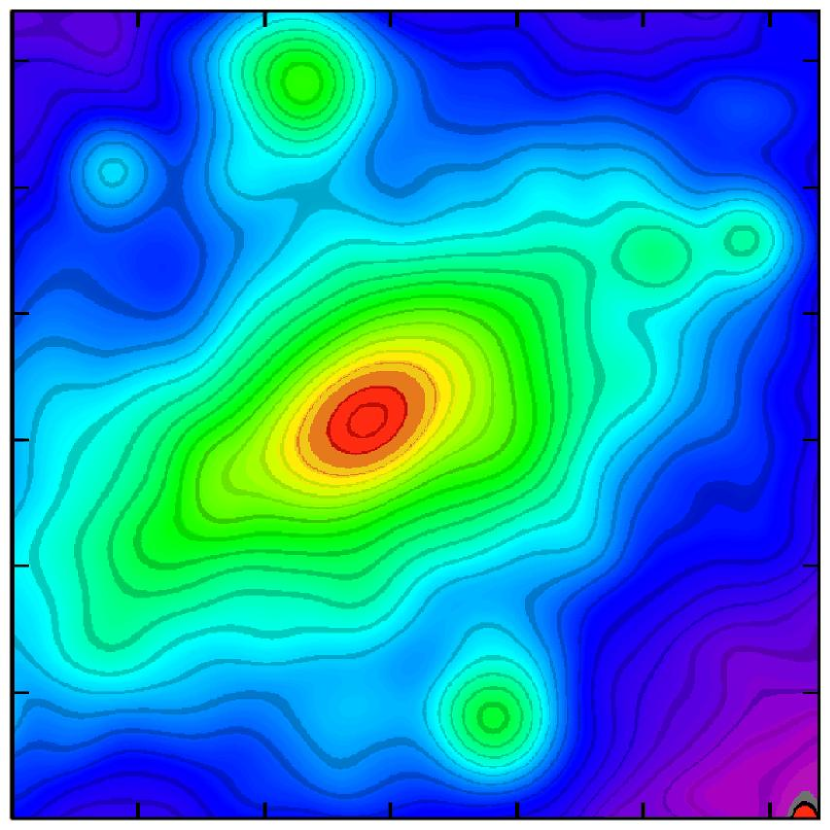
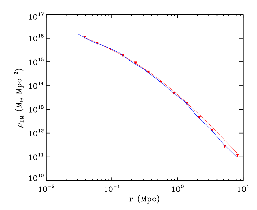
Figure 16.— Comparison with the Santa Barbara cluster (Frenk et al., 1999). The left panel shows the projected dark matter density at $z=0$. The image, covering the inner 8 Mpc of the simulation cube, has been smoothed with a Gaussian kernel of $R_{\rm G}=250$ kpc. The right panel shows the radial spherical density distribution for the halo (red triangles), together with the mean points from the Santa Barbara project (blue line). The red line indicates the best NFW fit to the data points.

Appendix B Comparison of the FTM code with the Santa Barbara Cluster

“The Santa Barbara cluster comparison project” (Frenk et al., 1999) was envisioned as a reliable comparison test between different cosmological numerical codes. It represents a hydrodynamical simulation of the formation of a rich cluster of galaxies. This exercise has become a standard test for new numerical codes in order to check for broad consistencies with other codes. Here we limit ourself to present only a comparison with respect to the DM properties of such cluster. The FTM has been tested extensively with respect to other dynamical codes.

We have simulated the Santa Barbara cluster with a numerical resolution of $128^{3}$ particles with a homogeneous sampling from the original $256^{3}$ realization. The left-panel of Figure 16 shows a density cut of the final output time from the simulation. This figure has been constructed in the same way as those presented in Frenk et al. (1999), i.e., , the image covers the inner 8 Mpc of the simulation cube, and it has been smoothed with a Gaussian kernel of $R_{\rm G}=250$ kpc. A visual comparison shows that our simulation possesses the same characteristics as the Santa Barbara one. This is further corroborated with the computed virial quantities: $M_{\rm vir}=1.06\times 10^{15}~{}M_{\odot}$, $R_{\rm vir}=2.63$ Mpc, which are in good agreement with those reported in the Santa Barbara project. In the right panel of Fig. 16 the radial density distribution of our cluster is presented. The red triangles represent our measurements and the red line shows the corresponding NFW profile. This distribution is in good agreement with respect to the averaged density profile reported in the Santa Barbara project.

References

- Allgood et al. (2006) Allgood, B., Flores, R. A., Primack, J. R., Kravtsov, A. V., Wechsler, R. H., Faltenbacher, A., & Bullock, J. S. 2006, MNRAS, 367, 1781
- Ascasibar et al. (2004) Ascasibar, Y., Yepes, G., Gottlöber, S., & Müller, V. 2004, MNRAS, 352, 1109
- Avila-Reese et al. (2005) Avila-Reese, V., Colín, P., Gottlöber, S., Firmani, C., & Maulbetsch, C. 2005, ApJ, 634, 51
- Barnes & Efstathiou (1987) Barnes, J. & Efstathiou, G. 1987, ApJ, 319, 575
- Barnes & Hut (1986) Barnes, J. & Hut, P. 1986, Nature, 324, 446
- Berentzen & Shlosman (2006) Berentzen, I. & Shlosman, I. 2006, ApJ, 648, 807
- Bertschinger (1985) Bertschinger, E. 1985, ApJS, 58, 39
- Bertschinger (1987) —. 1987, ApJ, 323, L103
- Binney (2004) Binney, J. 2004, MNRAS, 350, 939
- Bistolas & Hoffman (1998) Bistolas, V. & Hoffman, Y. 1998, ApJ, 492, 439
- Blais-Ouellette et al. (2001) Blais-Ouellette, S., Amram, P., & Carignan, C. 2001, AJ, 121, 1952
- Bolatto et al. (2002) Bolatto, A. D., Simon, J. D., Leroy, A., & Blitz, L. 2002, ApJ, 565, 238
- Broadhurst et al. (2005) Broadhurst, T., Takada, M., Umetsu, K., Kong, X., Arimoto, N., Chiba, M., & Futamase, T. 2005, ApJ, 619, L143
- Bullock et al. (2001a) Bullock, J. S., Dekel, A., Kolatt, T. S., Kravtsov, A. V., Klypin, A. A., Porciani, C., & Primack, J. R. 2001a, ApJ, 555, 240
- Bullock et al. (2001b) Bullock, J. S., Kolatt, T. S., Sigad, Y., Somerville, R. S., Kravtsov, A. V., Klypin, A. A., Primack, J. R., & Dekel, A. 2001b, MNRAS, 321, 559
- Cole & Lacey (1996) Cole, S. & Lacey, C. 1996, MNRAS, 281, 716
- Davis et al. (1985) Davis, M., Efstathiou, G., Frenk, C. S., & White, S. D. M. 1985, ApJ, 292, 371
- de Blok & Bosma (2002) de Blok, W. J. G. & Bosma, A. 2002, A&A, 385, 816
- Dehnen (2002) Dehnen, W. 2002, J. Comp. Phys., 27
- Dehnen (2005) —. 2005, MNRAS, 360, 892
- Diemand et al. (2004) Diemand, J., Moore, B., Stadel, J., & Kazantzidis, S. 2004, MNRAS, 348, 977
- Eisenstein & Hut (1998) Eisenstein, D. J. & Hut, P. 1998, ApJ, 498, 137
- Eke et al. (2001) Eke, V. R., Navarro, J. F., & Steinmetz, M. 2001, ApJ, 554, 114
- El-Zant (2005) El-Zant, A. 2005, astro-ph/0502472
- El-Zant et al. (2001) El-Zant, A., Shlosman, I., & Hoffman, Y. 2001, ApJ, 560, 636
- El-Zant et al. (2004) El-Zant, A. A., Hoffman, Y., Primack, J., Combes, F., & Shlosman, I. 2004, ApJ, 607, L75
- Fillmore & Goldreich (1984) Fillmore, J. A. & Goldreich, P. 1984, ApJ, 281, 1
- Flores & Primack (1994) Flores, R. A. & Primack, J. R. 1994, ApJ, 427, L1
- Frenk et al. (1999) Frenk, C. S., White, S. D. M., Bode, P., Bond, J. R., Bryan, G. L., Cen, R., Couchman, H. M. P., Evrard, A. E., Gnedin, N., Jenkins, A., Khokhlov, A. M., Klypin, A., Navarro, J. F., Norman, M. L., Ostriker, J. P., Owen, J. M., Pearce, F. R., Pen, U.-L., Steinmetz, M., Thomas, P. A., Villumsen, J. V., Wadsley, J. W., Warren, M. S., Xu, G., & Yepes, G. 1999, ApJ, 525, 554
- Fukushige & Makino (1997) Fukushige, T. & Makino, J. 1997, ApJ, 477, L9+
- Fukushige & Makino (2003) —. 2003, ApJ, 588, 674
- Gardner (2001) Gardner, J. P. 2001, ApJ, 557, 616
- Gelb & Bertschinger (1994) Gelb, J. M. & Bertschinger, E. 1994, ApJ, 436, 467
- Gentile et al. (2004) Gentile, G., Salucci, P., Klein, U., Vergani, D., & Kalberla, P. 2004, MNRAS, 351, 903
- Ghigna et al. (2000) Ghigna, S., Moore, B., Governato, F., Lake, G., Quinn, T., & Stadel, J. 2000, ApJ, 544, 616
- Gunn (1977) Gunn, J. E. 1977, ApJ, 218, 592
- Gunn & Gott (1972) Gunn, J. E. & Gott, J. R. I. 1972, ApJ, 176, 1
- Heller (1995) Heller, C. H. 1995, ApJ, 455, 252
- Heller & Shlosman (1994) Heller, C. H. & Shlosman, I. 1994, ApJ, 424, 84
- Hernquist (1990) Hernquist, L. 1990, ApJ, 356, 359
- Hiotelis (2002) Hiotelis, N. 2002, A&A, 382, 84
- Hoekstra et al. (2004) Hoekstra, H., Yee, H. K. C., & Gladders, M. D. 2004, ApJ, 606, 67
- Hoffman & Ribak (1991) Hoffman, Y. & Ribak, E. 1991, ApJ, 380, L5
- Hoffman & Shaham (1985) Hoffman, Y. & Shaham, J. 1985, ApJ, 297, 16
- Jing & Suto (2000) Jing, Y. P. & Suto, Y. 2000, ApJ, 529, L69
- Jing & Suto (2002) —. 2002, ApJ, 574, 538
- Klypin et al. (2001) Klypin, A., Kravtsov, A. V., Bullock, J. S., & Primack, J. R. 2001, ApJ, 554, 903
- Kravtsov et al. (2002) Kravtsov, A. V., Klypin, A., & Hoffman, Y. 2002, ApJ, 571, 563
- Lemson & Kauffmann (1999) Lemson, G. & Kauffmann, G. 1999, MNRAS, 302, 111
- Łokas & Hoffman (2000) Łokas, E. L. & Hoffman, Y. 2000, ApJ, 542, L139
- Lu et al. (2006) Lu, Y., Mo, H. J., Katz, N., & Weinberg, M. D. 2006, MNRAS, 368, 1931
- Macciò et al. (2003) Macciò, A. V., Murante, G., & Bonometto, S. P. 2003, ApJ, 588, 35
- Moore et al. (1998) Moore, B., Governato, F., Quinn, T., Stadel, J., & Lake, G. 1998, ApJ, 499, L5+
- Moore et al. (1999) Moore, B., Quinn, T., Governato, F., Stadel, J., & Lake, G. 1999, MNRAS, 310, 1147
- Navarro et al. (1997) Navarro, J. F., Frenk, C. S., & White, S. D. M. 1997, ApJ, 490, 493
- Nusser (2001) Nusser, A. 2001, MNRAS, 325, 1397
- Nusser & Sheth (1999) Nusser, A. & Sheth, R. K. 1999, MNRAS, 303, 685
- Padmanabhan (1993) Padmanabhan, T. 1993, Structure Formation in the Universe (Structure Formation in the Universe, by T. Padmanabhan, pp. 499. ISBN 0521424860. Cambridge, UK: Cambridge University Press, June 1993.)
- Peebles (1969) Peebles, P. J. E. 1969, ApJ, 155, 393
- Peirani et al. (2004) Peirani, S., Mohayaee, R., & de Freitas Pacheco, J. A. 2004, MNRAS, 348, 921
- Reed et al. (2005a) Reed, D., Governato, F., Quinn, T., Gardner, J., Stadel, J., & Lake, G. 2005a, MNRAS, 359, 1537
- Reed et al. (2005b) Reed, D., Governato, F., Verde, L., Gardner, J., Quinn, T., Stadel, J., Merritt, D., & Lake, G. 2005b, MNRAS, 357, 82
- Ricotti (2003) Ricotti, M. 2003, MNRAS, 344, 1237
- Romano-Díaz (2004) Romano-Díaz, E. 2004, PhD thesis, University of Groningen, Kapteyn Astronomical Institute
- Romano-Díaz et al. (2006) Romano-Díaz, E., Faltenbacher, A., Jones, D., Heller, C., Hoffman, Y., & Shlosman, I. 2006, ApJ, 637, L93
- Ryden (1988) Ryden, B. S. 1988, ApJ, 329, 589
- Ryden & Gunn (1987) Ryden, B. S. & Gunn, J. E. 1987, ApJ, 318, 15
- Salucci & Burkert (2000) Salucci, P. & Burkert, A. 2000, ApJ, 537, L9
- Shaw et al. (2005) Shaw, L., Weller, J., Ostriker, J. P., & Bode, P. 2005, astro-ph/0509856
- Simon et al. (2003) Simon, J. D., Bolatto, A. D., Leroy, A., & Blitz, L. 2003, ApJ, 596, 957
- Simon et al. (2005) Simon, J. D., Bolatto, A. D., Leroy, A., Blitz, L., & Gates, E. L. 2005, ApJ, 621, 757
- Springel et al. (2001) Springel, V., White, S. D. M., Tormen, G., & Kauffmann, G. 2001, MNRAS, 328, 726
- Steinmetz & Bartelmann (1995) Steinmetz, M. & Bartelmann, M. 1995, MNRAS, 272, 570
- Subramanian et al. (2000) Subramanian, K., Cen, R., & Ostriker, J. P. 2000, ApJ, 538, 528
- Syer & White (1998) Syer, D. & White, S. D. M. 1998, MNRAS, 293, 337
- Tasitsiomi et al. (2004) Tasitsiomi, A., Kravtsov, A. V., Gottlöber, S., & Klypin, A. A. 2004, ApJ, 607, 125
- Taylor & Navarro (2001) Taylor, J. E. & Navarro, J. F. 2001, ApJ, 563, 483
- van de Weygaert & Bertschinger (1996) van de Weygaert, R. & Bertschinger, E. 1996, MNRAS, 281, 84
- van den Bosch (2002) van den Bosch, F. C. 2002, MNRAS, 331, 98
- Vitvitska et al. (2002) Vitvitska, M., Klypin, A. A., Kravtsov, A. V., Wechsler, R. H., Primack, J. R., & Bullock, J. S. 2002, ApJ, 581, 799
- Warren et al. (1992) Warren, M. S., Quinn, P. J., Salmon, J. K., & Zurek, W. H. 1992, ApJ, 399, 405
- Wechsler et al. (2002) Wechsler, R. H., Bullock, J. S., Primack, J. R., Kravtsov, A. V., & Dekel, A. 2002, ApJ, 568, 52
- Wechsler et al. (2005) Wechsler, R. H., Zentner, A. R., Bullock, J. S., Kravtsov, A. V., & Allgood, B. 2005, astro-ph/0512416
- Weinberg & Katz (2002) Weinberg, M. D. & Katz, N. 2002, ApJ, 580, 627
- Weldrake et al. (2003) Weldrake, D. T. F., de Blok, W. J. G., & Walter, F. 2003, MNRAS, 340, 12
- Zaroubi & Hoffman (1993) Zaroubi, S. & Hoffman, Y. 1993, ApJ, 416, 410
- Zel’dovich (1970) Zel’dovich, Y. B. 1970, A&A, 5, 84
- Zhao et al. (2003) Zhao, D. H., Mo, H. J., Jing, Y. P., & Börner, G. 2003, MNRAS, 339, 12
- Zhao (1996) Zhao, H. 1996, MNRAS, 278, 488