The Mass Distribution of the Central Stars of Planetary Nebulae in the Large Magellanic Cloud

Abstract

We present the properties of the central stars from a sample of 54 Planetary Nebulae (PNe) observed in the Large Magellanic Cloud (LMC) with the Hubble Space Telescope Imaging Spectrograph (STIS). The Hubble Space Telescope’s spatial resolution allows us to resolve the central star from its nebula (and line-of-sight stars) at the distance of the LMC, eliminating the dependency on photoionization modeling in the determination of the stellar flux. For the PNe in which the central star is detected we obtain the stellar luminosities by directly measuring the stellar fluxes through broad-band imaging and the stellar temperatures through Zanstra analysis. From the position of the central stars in the HR diagram with respect to theoretical evolutionary tracks, we are able to determine reliable core masses for 21 central stars. By including the central star masses determined in this paper to the 16 obtained previously using the same technique (Villaver et al., 2003), we have increased the sample of central star masses in the LMC to 37, for which we find a non-Gaussian mass distribution. The average central star mass for this sample is $<m_{CS},LMC>$ = 0.65$\pm$0.07 M_⊙, slightly higher than the one reported in the literature for both white dwarfs and the central stars of PNe in the Galaxy. If significant, this higher average central star mass in the LMC can be understood in terms of a metallicity dependency on mass-loss rates during the Asymptotic Giant Branch, since the LMC has on average half the metallicity compared to the Galaxy. Finally, for the 37 objects analyzed in the LMC, we do not find any significant correlation between the mass of the central star and the morphology of the nebula.

1 INTRODUCTION

The central stars of Planetary Nebulae (PNe) are the result of the evolution of stars in the approximate mass range 1–8 M_⊙ that ascend the Asymptotic Giant Branch (AGB) after both hydrogen and helium have been exhausted in the core. The heavy, and largely unknown, mass-loss rates taking place during the late AGB evolution (Willson, 2000) ultimately determine the initial–to–final mass relation for single stars and therefore the mass boundary between those stars that will evolve off the AGB phase into central stars of PNe and ultimately fade into white dwarfs, and those that will end their lives as Type ii Supernovae.

After the star leaves the AGB, it first evolves into the PN phase at constant luminosity towards higher effective temperatures following an evolutionary track that is mostly dependent on the central star mass. The mass of the central star alone determines the energy budget and the timescale of evolution of the nebular shell (Villaver et al., 2002b). An accurate measurement of the central star properties (mass, effective temperature and luminosity) is then crucial to understanding how the formation and evolution of PNe relates to the initial mass of the progenitor star. Moreover, central stars of PNe are the immediate stellar precursors of white dwarfs and in principle the determination of their masses should provide further constraints to fundamental empirical quantities such as the initial–final mass relation which rely primarily on the measurements of white dwarfs masses. Although the central stars of PNe can be up to 10⁴ times more luminous than white dwarfs, their mass determination in our Galaxy is extremely uncertain (i.e. Shaw & Kaler 1989; Stanghellini et al. 2000) primarily due to the poor knowledge of their individual distances. The central star evolutionary tracks in the HR diagram depend primarily on mass and show very little variation with the central star luminosity. In the best case scenario, the horizontal part of the HR diagram, the dependency of the central star mass ($M_{CS}$) with its luminosity ($L_{CS}$) goes as, $[M_{CS}/M_{\rm\odot}]~{}=~{}0.5+1.8\times 10^{-5}~{}[L_{CS}/L_{\rm\odot}]$ (Vassiliadis & Wood, 1994) which means that in order to determine accurately the central star mass the distance has to be known to better than 10% (Shaw, 2006).

In principle the problem with the distance uncertainties can be overcome by observing PNe in the Magellanic Clouds, where the distance is known to an accuracy of $\sim$10% (Benedict et al., 2002), and the distances to all nebulae within one Cloud are known to within a few percent. However, since PNe in the Magellanic Clouds cannot be resolved using ground-based observations, the central star parameters derived from ground–based studies have usually relied heavily on photoionization modeling of the nebula (Boroson, & Liebert, 1989; Henry, Liebert, & Boroson, 1989; Dopita, Meatheringham, 1991a, b; Meatheringham & Dopita, 1991a, b). As a result, these studies can only determine lower limits to the stellar luminosities (Villaver, 2006). The high spatial resolution capabilities of the Hubble Space Telescope (HST) allowed for the first time to spatially resolve PNe in the Magellanic Clouds. The first HST observations of PNe in the Magellanic Clouds, however, were designed to target the nebulae through narrow-band filters (Dopita et al., 1994, 1996, 1997; Vassiliadis et al., 1996, 1998) and since they could not detect the central star, they did not yield a significant improvement in the determination of the central star parameters compared to results based on ground-based observations.

Our group has acquired and analyzed the first HST data samples of PNe in the Magellanic Clouds, aimed at determining the stellar continuum through broad-band imaging (Shaw et al., 2001; Stanghellini et al., 2002a). The first detailed analysis of the central stars included a sample of 35 PNe in the Large Magellanic Cloud (LMC) (Villaver et al., 2003) and 27 PNe in the Small Magellanic Cloud (SMC) (Villaver et al., 2004). Often the central star is not detected above the nebular continuum, either because it has evolved to luminosities below our detection limits or because the nebular continuum is brighter than the stellar one. As a consequence the properties of only 14 (out of 27 PNe observed in the SMC) and 16 (out of 35 PNe in the LMC) central stars were determined. Note that only four masses of central stars in the LMC were known previously from direct measurement of the stellar flux (Dopita et al., 1993; Bianchi, Vassiliadis, & Dopita, 1997) (seven more central star masses have been determined in the LMC since then by Herald & Bianchi 2004). From the analysis of our HST samples we found an average central star mass of 0.63$\pm$0.1 M_⊙ in the SMC (Villaver et al., 2004), which is similar to the average mass obtained in the LMC (0.65$\pm$0.07 M_⊙) (Villaver et al., 2003). However, we found that the SMC and LMC central star mass distributions are different, in that the SMC sample lacks an intermediate-mass stellar population (0.65 to 0.75 M_⊙) (Villaver et al., 2004).

In this paper, we extend our previous study of the properties of the LMC central stars to a sample of 54 additional PNe. We present the analysis of the central stars of PNe obtained on a Cycle 10 HST SNAPSHOT survey of LMC PNe using broad-band imaging with the Space Telescope Imaging Spectrograph (STIS). The broad and narrow-band images of the PNe are presented elsewhere (Shaw et al., 2006), together with the line intensities and nebular physical conditions obtained by using HST STIS slitless spectroscopy. In §2 we describe the observations and in §3 the photometric calibration, and the central star temperature and luminosity determinations. Our results are presented in §4 and discussed and summarized in §5.

2 OBSERVATIONS

The observations presented in this paper are from the HST program #9077 (P.I. Shaw). The targets were scheduled as SNAPSHOT exposures, which means that the actual observations were selected on the basis of expediency for the scheduling system, and on the availability of visits with suitable durations. The observation log, observing configuration, target selection, acquisition and a description of the basic calibration (through flat-fielding) can be found in Shaw et al. (2006). The target list included all known LMC PNe that have not already been observed with HST and was derived from the catalogs of Sanduleak et al. (1978), Sanduleak (1984), Jacoby (1980), Morgan & Good (1992) and Morgan (1994).

The photometry of the central stars has been obtained from the STIS clear aperture mode images (50CCD). The 50CCD is an unvigneted aperture with a field of view of 52″$\times$ 52″  and a focal plate scale of 0″.0507 pix^-1. In this setting no filter is used and the shape of the bandpass is governed by the detector (which has a sensitivity from $\sim$2 000 to 10 300 Å) and by the reflectivity of the optics. The central wavelength of the 50CCD is 5850Å, and the bandpass is 4410 Å. The FWHM of the PSF is close to 2 pixels at 5 000 Å and the 90% encircled energy radius is 3 pixels (Leitherer et al., 2001). The observations were made with the CCD detector using a gain of 1 $e^{-}$ per analog-to-digital converter unit. All the exposures were split into two equal components to allow cosmic-ray rejection.

Table 1 gives in column (1) the object name according to the SMP nomenclature when available, in columns (2) and (3) the sky coordinates, in column (4) the nebular diameters measured with respect to the 10% intensity contour of the outer most structure in the [O iii] 5007 Å line, in column (5) the total integration time, and in column (6) whether or not the central star was detected in the images.

3 ANALYSIS

3.1 Stellar Photometry

The photometric technique has already been described in detail in Villaver et al. (2003). In summary, we have applied aperture photometry using the IRAF PHOT task. Given the spatially resolved nature of the nebula we measure the flux within a circular aperture with a radius of 2 pixels centered on the star, and subtract the nebular emission by estimating the median nebular flux in an annulus with a width of 1 or 2 pixels adjacent to the stellar aperture. The nebular emission within this aperture can be highly inhomogeneous and strong variations from the median of the nebular flux are reflected in the large standard deviation. These uncertainties are propagated into the errors of the measured magnitudes. The internal consistency of the procedure, which is accurate at the 1% level, has been tested in previous papers by performing aperture photometry on nebular subtracted images built by co-adding 2D monochromatic images taken from the STIS spectroscopy.

The instrumental magnitudes are given in the STMAG system by using the zero-point calibration and aperture corrections presented in Brown et al. (2002). The STIS charge transfer efficiency (CTE) correction was applied in this version of the pipeline (see Shaw et al. 2006) but it has been shown only to have an effect less than 0.01 mags (Rejkuba et al., 2000) for stars in the center of the field.

The stellar extinction correction has been estimated from the nebular Balmer decrement, c, and the relation $c~{}=~{}1.41~{}E_{B-V}$ (Seaton, 1979), where E_B-V is the color excess. Ultimately this approach relies on the lack of strong spatial variations in the extinction within the nebula caused by internal absorption by dust. Significant spatial variations in the H$\beta$/H$\alpha~{}$ratio within the nebulae have not been found for any of the heavily reddened objects in our sample, confirming the validity of this approach. The extinction constants have been taken from (Shaw et al., 2006) except for J 5, MG 16 and MO 33 where the extinction could not be determined because the intensity of the H$\alpha~{}$line was blended with the [N ii] 6548, 6583 Å line emission in the slitless spectra. The extinction constants for J 5, MG 16, and MO 33 are not available in the literature and therefore we have assumed zero extinction for these central stars. Note that the mean extinction for the bright Magellanic Cloud PNe observed with the HST is $c~{}=~{}$0.19 (Shaw, 2006) so adopting a low extinction for this purpose is not unreasonable.

In the wavelength range under consideration, the LMC and Galactic extinction laws are very similar (Howarth, 1983). Thus, we used the interstellar extinction law of Savage & Mathis (1979) and assumed that R${}_{V}~{}=~{}3.1$. The extinction in magnitudes (A_V) is then A${}_{V}~{}=~{}2.2c$.

The transformation from the instrumental STMAG magnitude to the standard V-band magnitude in the photometric Johnson-Cousins UBVI system has been derived using synthetic photometry with IRAF/STSDAS SYNPHOT by using a blackbody spectrum to represent the Spectral Energy Distribution (SED) of the central star. The procedure, which is described in detail in Villaver et al. (2003), basically consists in obtaining a median of the V-50CCD colors for blackbodies between 30 000 and 300 000  K with the extinction values appropriate for each source. The uncertainty in the transformation has been added in quadrature to the error in the measured magnitude.

When the central star is not detected (i.e., no stellar PSF appears above the nebular level), we computed a lower limit to the central star magnitude by measuring the flux inside a stellar aperture at the geometric center of the nebula (i.e., the most likely position of the central star). The lower limits to the magnitudes for those central stars that have not been detected in our sample are presented in Table 2 where column (1) gives the object name, columns (2) and (3) give the lower limit magnitude of the central star in the STMAG and Johnson-Cousins systems respectively and column (4) gives the nebular extinction constant.

In Table 3, we give the results of the photometry for the objects in which the central star has been detected. Column (1) gives the PN name, columns (2) and (3) give the STMAG and $V$ magnitudes respectively as well as the associated errors. The uncertainties includes the CCD noise (i.e. photon noise and read noise), the systematic error (central star flux, sky) and the errors in the calibration. The nebular extinction constants used to correct for the stellar extinction are listed in column (4). We have 6 objects (MG 29, Mo 47, Sa 121, SMP 45, SMP 49, and SMP 74) for which the central star is detected, but at a marginal level above the nebula (see footnote in Table 1). The large errors obtained for these objects directly reflect the uncertainty in the measurement of the stellar magnitude.

3.2 Effective Temperatures, Bolometric Corrections and Stellar Luminosities

As in previous papers we have estimated the temperature of the central star by using the method originally developed by Zanstra (Zanstra, 1931) which is extensively used in the literature (i.e. Harman & Seaton 1966; Kaler 1983; Stanghellini et al. 2002b). The Zanstra temperature is an estimate of the ionizing flux from a star computed by comparing the flux of a nebular recombination line of hydrogen or helium to the stellar continuum flux in the $V$-band assuming a particular choice for the stellar spectral energy distribution, which in our case is a blackbody.

The data needed for the temperature calculation have been taken from Shaw et al. (2006) (H$\beta$ fluxes, nebular radii and extinction constants). The He ii 4686 Å line fluxes were taken from Boroson, & Liebert (1989), Meatheringham & Dopita (1991a), Morgan & Parker (1998), and Leisy & Dennefeld (2006). In order to assure the best results we have been very conservative with the uncertainties in the fluxes quoted by the references. We have supplemented the above with fluxes from our unpublished, ground-based NTT spectra for SMP 57. In Table 3, column (5) we list the He ii 4686 Å line intensity relative to H$\beta$ = 100, not corrected for extinction; in column (6) we list the reference code for the He ii 4686 Å fluxes.

The bolometric correction (BC) dependence with stellar effective temperature was taken from Vacca, Garmany, & Shull (1996) which was derived for Galactic O-type and early B-type stars. We use this relation because the dependence of BC with $\log$ g was found to be extremely weak. The BCs have been computed by using the He ii Zanstra temperature when available, otherwise the H i Zanstra temperature was used. Temperatures derived from He ii Zanstra analysis are the most reliable, because most PNe are optically thick to He ii ionizing photons. H i Zanstra temperatures can be reliable for PNe with sufficient optical depth, but the problem is in determining which PNe are optically thick to hydrogen ionizing radiation.

In order to compute the central star luminosities we adopted a distance to the LMC of 50.6 kpc and an absolute bolometric magnitude for the Sun of M_bol,⊙= 4.75 mag (Allen, 1976). Note that the same distance to the LMC is used by the HST Key Project in the extragalactic distance scale (Freedman et al., 2001; Mould et al., 2000). From the three dimensional structure of the LMC (Freeman, Illingworth, & Oemler, 1983; van der Marel & Cioni, 2001), we have estimated a spread in the distance modulus of 0.03, which we propagate into the error of the absolute magnitudes and luminosities. We have not taken into account the error in the distance to the LMC, because it will affect all the objects in the same way.

We give the computed temperatures and luminosities in Table 4. In column (1) we give the PN name; in columns (2) and (3) we give the effective temperatures (in units of 10³ K) derived from the Zanstra method for the He ii and for the H i recombination lines, respectively. The visual absolute magnitudes derived from the BCs are listed in column (4). The BCs and their errors, computed by propagating the errors in the determination of the effective temperature are given in column (5). Column (6) gives the stellar luminosity and column (7) the morphological classification of the PN. We use the morphological classification of the nebula given in Shaw et al. (2006). PNe are classified as Round, Elliptical, Bipolar, and Point-symmetric according to their morphology in the [O iii] 5007 Å line. We have excluded the bipolar core morphological class as a secondary morphology indicator given the small number of objects with bipolar core morphology and with detected central stars.

4 RESULTS

4.1 Central Star Direct Detection

We are able to detect and successfully measure a central star magnitude in 64% of all PNe presented in this paper, and in Villaver et al. (2003, 2004). When we are unable to measure the central star magnitude, the most common reason is that the nebular continuum is much stronger than that from the central star. This is illustrated in Figure 1, where we plot the stellar $V$ magnitudes vs. the average surface brightness of the PN in H$\beta$ emission. The nebular continuum is primarily composed of free-bound emission from H⁰ and He⁺ (when present), although free-free emission can be a significant contributor in the blue part of the spectrum (Osterbrock, 1989). This emission will for the most part be spatially coincident with the H bound-bound emission. One would expect that the stellar magnitudes would be well determined above the noise, and less well determined or undetected as the stellar continuum becomes lost in the nebula. This is clear from Fig. 1, where the error bars on the magnitudes increase along the upper envelope of the trend line until all that can be determined is a lower limit. The transition region between well determined magnitudes and limits is not perfectly sharp because the nebular continuum is often spatially non-uniform, which can but often does not necessarily complicate the photometry. Stars shown as upper limits are those where the central star was saturated in the image. Stars with very faint lower limits are those that were not detectable even in the absence of nebular continuum.

In all, the technique of observing the central stars of PNe with the STIS 50CCD aperture has been very effective and yields an accurate $V$ magnitude for most of the time. In cases where the stars are undetectable, useful limits can be set on the stellar flux. In addition, the high-resolution image (see Shaw et al. 2006) provides a clear view of the proximity of field stars from which the viability of ground-based observations of the central star can be judged. Very often it is the central stars of bipolar nebulae that are lost in the continuum of the surrounding nebula, which limits our ability to study the evolution of their progenitors. In order to improve significantly on our technique for detecting the central star directly, it will be necessary either to obtain high quality spectra and model the nebular continuum, or to obtain high-resolution images of these PNe in the ultraviolet.

As mentioned in the introduction, in the past, most of the central star properties of PNe in the LMC and SMC have been derived from ground-based optical spectroscopic observations that do not permit a separation of the stellar continuum from that of the nebula. As a result, the central star luminosity and temperature have to be computed using modeling techniques that rely completely on nebular measurements. The strongest implications of this approach is on the stellar luminosities that are determined from the H$\beta$ line flux of the nebula under the assumption that the nebula is optically thick. The nebular H$\beta$ line flux is used as a measurement of the recombination and therefore the ionizing flux from the star. The main problem with this approach of estimating the stellar luminosity is that the nebulae are sometimes totally optically thin, or thin in some directions, and therefore the derived stellar luminosities are lower limits.

4.2 Stellar Distribution on the $\rm\log\,L-\log\,T$ Plane

In Figure 2 we show the distribution in the $\rm\log\,L-\log\,T$ plane of the central stars analyzed in this paper. In the cases where the flux at He ii 4686 Å was not available (MG 16, Mo 7, Mo 33, SMP 43, and Mo 47), we have used the H i Zanstra temperature to locate the central stars on the HR diagram. It is well known that the H i Zanstra temperature underestimates the temperature of the central stars of optically thin PNe (i.e. Kaler & Jacoby 1989; Gruenwald & Viegas 2000) but it is accurate for optically thick objects. We have also used H i Zanstra temperatures for J 39 that has zero measured flux at He ii 4686 Å and for SMP 67 where the measured He ii 4686 Å flux is very small and therefore the uncertainty is expected to be very high.

Figure 3 shows the distribution in the $\rm\log\,L-\log\,T$ plane of the total sample of central stars observed by us with HST in the LMC. The central star parameters obtained in Villaver et al. (2003) from HST GO program 8271 (Shaw et al., 2001) for 16 central stars have been added to the 21 central stars shown in Fig. 2. We see an identical distribution of the central star locations in the HR diagram when we plot the two samples together and in either sample we do not find any central star with an effective temperature below 30 000  K. From stellar evolution theory a massive progenitor would evolve very fast along this region of the HR diagram and therefore the probability of detection is very small. From numerical simulations coupled to the central star evolution (Villaver et al., 2002a, b), a very low-mass central star, although it evolves more slowly in the HR diagram, it still needs at least 3 000  yr (after the star leaves the AGB) for a thin PN shell to become ionized and therefore observable. Shorter timescales than $\sim$3 000  yr are needed to observe ionized PNe originating from intermediate-mass progenitors (Villaver et al., 2002b). We believe that the coupled evolution between the star and the nebula is reflected in the location of the central stars in the HR diagram shown in Fig. 3.

The central star masses obtained in this paper have been derived from Fig. 2 by comparing their location on the HR diagram with the Vassiliadis & Wood (1994) tracks for stars with LMC metallicity (Z = 0.008). Note that the progenitors of the PNe we studied have a range of initial metallicities, and using single metallicities for all the tracks has the potential to introduce additional uncertainty in the determination of individual masses. We have not plotted or derived masses for the stars that lie below the evolutionary tracks (MG 14, MG 16, Mo 7, Sa 117 and Mo 47). We did not have He ii 4686 Å fluxes (or the He ii 4686 Å  measured flux is very small) for MG 14, MG 16, Mo 7 and Mo 47 and therefore their central star parameters are very uncertain. The central star of Sa 117 is only marginally detected above the nebula. We did not estimate the central star masses for MG 45, Sa 104a, and SMP 88 that have much larger luminosities than those encompassed by the highest mass evolutionary track. Given the compact nature of these three PNe, our photometric technique fails in subtracting the true nebular contribution from the stellar aperture. J 5 has been excluded as well from the following analysis because its magnitude was measured from saturated data and because most of its Balmer emission appears to be coming from the central star (Shaw et al., 2006). The core masses and the morphological classification of the nebulae are summarized in Table 5.

The Vassiliadis & Wood (1994) LMC models are more efficient at producing He-burning post-AGB tracks for lower mass progenitors, which they argue is a natural consequence of the mass-loss behavior during the AGB phase. The He-burning or H-burning nature of the post-AGB track depends on whether the star leaves the AGB when helium-shell or when hydrogen-shell burning is dominant. However, the mechanism that controls the departure of the star from the AGB is unknown and therefore artificially defined in the stellar evolutionary models. From our data we cannot constrain the nature of the track, so when possible we have estimated the masses from both the H-burning and the He-burning LMC tracks.

Note that the central star temperatures and luminosities (and therefore the masses) have been computed under the assumption of a non-binary central star, i.e. assuming that all the measured flux arises from the central star. The reliability of this assumption has been addressed in Villaver et al. (2004) where we explored the possibility of light from a stellar companion contaminating the photometric measurements. A significant contribution from a stellar companion to the measured flux in the STIS/50CCD bandpass can be excluded given the additional restriction that a known distance imposes on the measured flux. It is important to note that our analysis does not rule out the possibility of a binary companion to the central star: we only exclude companions with fluxes in the STIS bandpass that are comparable to that of the ionizing source.

4.3 Central Star Mass-PN Morphology Relation

Given the large amount of observational evidence that shows fundamental differences in the physical and chemical properties among PN morphological classes, it has been suggested that the initial mass of the progenitor star determines the morphology of the PN. In particular, the N and O chemical enrichment found in the Galactic bipolar and extremely asymmetric morphological classes (Greig, 1971; Peimbert, 1978; Torres-Peimbert & Peimbert, 1997) together with their lower average distance from the Galactic plane (Corradi & Schwarz, 1995; Manchado et al., 2000; Stanghellini et al., 2002b; Parker et al., 2006), suggests that the bipolar class might evolve from more massive progenitors and given the initial–final mass relation massive progenitors imply massive central stars. The correlation between the central star mass and the PN morphology has been explored for Galactic samples by several authors (Stanghellini, Corradi, & Schwarz, 1993; Amnuel, 1995; Gorny, Stasinska, & Tylenda, 1997; Stanghellini et al., 2002b) who have found slightly different mass distributions for the central stars of symmetric and axisymmetric PNe. In the sample of objects analyzed in this paper, we do not find any correlation between the mass of the central star and the morphology of the nebula. The lack of correlation still holds if we include the LMC objects presented in Villaver et al. (2003). The number of objects with bipolar/quadrupolar morphology and central star masses measured is small (9 objects), although it still represents 24% of the sample of 37 objects. The average mass of the central stars of the 9 bipolar PNe is 0.64$\pm$0.04 M_⊙.

In assessing the lack of correlation found between central star mass and morphology in this sample, it is important to consider the various selection effects that may shape the outcome. Shaw et al. (2006) pointed out that the selection of objects to be imaged with HST is, for a variety of reasons, skewed towards brighter objects, and the completeness of faint PNe in the LMC at the time the HST targets were selected was poor compared to the SMC (Jacoby & De Marco, 2002). Note that the number of PNe known in the in the central 25 sq. degree region of the LMC, especially at the faint end, have just tripled (Reid & Parker, 2006). The incidence of bipolars is higher for less luminous PNe (Shaw et al., 2006), which suggests that bipolars might be under-represented in our sample. The detection rate of central stars in bipolar PNe is comparable to or only slightly less than that for the full sample. However, the reasons for failing to detect central stars seems to be different among the different morphological classes. While non-detected central stars in bipolar PNe are too faint, non-detected central stars in round and elliptical PNe are often buried in bright nebulosity (sometimes even saturated). Finally, one should recall that high-mass central stars evolve very quickly through the HR diagram, and therefore are most likely to be found at low luminosities. If bipolar nebulae are produced by high-mass progenitors, then they may fall below our detection limit more readily than central stars in other types of nebulae. The magnitude of these selection effects is hard to quantify and might play a role in the average central star mass determined for the bipolar class.

4.4 The LMC Central Star Mass Distribution

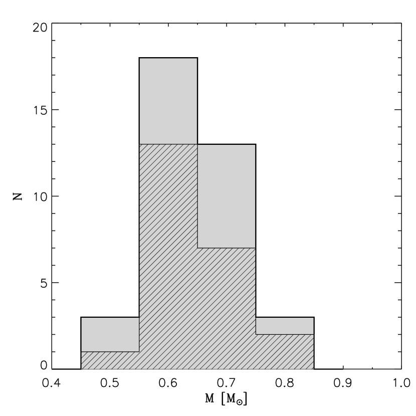
Figure 4: The gray histogram represents the central star mass distribution of the sample of objects analyzed by us in the LMC (i.e. masses obtained in Villaver et al. (2003) and this paper). The hatched histogram represents the mass distribution of selected central stars from the whole sample that have He ii Zanstra temperature determinations and masses derived from H-burning post-AGB tracks.

In Figure 4 we show the histogram of the mass distribution of the 37 central stars of PNe obtained by us in the LMC (in gray). We have plotted the central star masses obtained in this paper (21 objects) and the LMC central star masses from Villaver et al. (2003) (16 objects). In the theoretical PN luminosity function and other PN applications, the central star mass distribution is generally assumed to be Gaussian. A Kolmogorov-Smirnov test (Chakravarti, Laha, & Roy, 1967) has been applied to determine the likelihood that the sample has been drawn from a parent population whose underlying distribution is normal. The KS test rules out this possibility at the 87% confidence level. A similar result is obtained by applying the Shapiro-Wilk test (Shapiro & Wilk, 1965). In Villaver et al. (2003) using a smaller number of objects, we pointed out that the measured central star masses were not normally distributed. Here we corroborate this result using a larger sample.

The mean and the median of the mass distribution of the 37 central stars of PNe in the LMC are 0.65$\pm$0.07 and 0.64$\pm$0.06 M_⊙ respectively. Stanghellini et al. (2002b) analyzed a sample that contained $\sim$200 central stars of PNe in the Galaxy and found an average mass $<~{}M_{CS},GAL~{}>$ = 0.60$\pm$0.13 M_⊙. The distribution of white dwarf masses in the Galaxy is very narrow as well with a peak at $\sim$0.57 M_⊙ and a tail extending towards larger masses (Bergeron, Saffer, & Liebert, 1992; Finley, Koester, & Basri, 1997; Madej et al., 2004). However, it has been noted that the average mass of the white dwarf population should be used with caution, as it depends on the underlying distribution of masses which is a function of the temperature range covered by the sample (Finley, Koester, & Basri, 1997). More recently, Liebert et al. (2005) have analyzed a large sample of 350 white dwarfs from the Palomar Green Survey and found the $<M_{WD},GAL>$ = 0.603$\pm$0.134 M_⊙ in good agreement with the Stanghellini et al. (2002b) results. The average mass of the total sample of LMC central stars presented in Fig. 4 (37 objects) is slightly higher than the average mass of both white dwarfs and central stars of PNe in the Galaxy reported in the literature.

The central star mass depends mainly on the stellar mass during the Main-Sequence phase (hereafter, the initial mass), and on the mass-loss during the AGB phase. Mass-loss during the AGB phase has a strong dependency on metallicity as it is thought to be driven mainly by dust (Wood, 1979; Bowen, 1988). The dust formation process depends on the chemical composition of the gas: the lower the metallicity the smaller the amount of dust formed, and the lower the efficiency of the momentum transfer to the gas. Thus, low metallicity stars with dust-driven winds are expected to loose smaller amounts of matter (Winters et al., 2000) and therefore are expected to end-up with higher central star masses. It has been shown that mass-loss during the AGB phase can also occur in the absence of dust (Willson, 2000), but in this case the mass-loss efficiency is much lower. The metallicity of the LMC is on average half that of the solar mix (Russell & Bessell, 1989; Russell & Dopita, 1990). Therefore, it is well expected that the efficiency of mass-loss during the AGB phase will be reduced in the LMC. As a result a higher central star mass should be the outcome of the evolution for a given initial progenitor. If we believe the higher average central star mass of PNe we find in the LMC we might have the first observational evidence from PNe progenitors for reduced mass-loss rates in a lower metallicity environment. The consequences are very important in terms of galactic chemical enrichment, as a higher fraction of main sequence stars should reach the Chandrasekhar mass limit in the LMC than in the Galaxy (Umeda, Nomoto, Yamaoka, & Wanajo, 1999; Dominguez, Chieffi, Limongi, & Straniero, 1999; Girardi, Bressan, Bertelli, & Chiosi, 2000).

It is important to mention that higher masses are obtained from He-burning evolutionary tracks than from H-burning tracks. As mentioned in §4.2 the nature of the tracks in stellar evolution models depends on the artificially selected point of departure from the AGB, with different authors using different criteria. Since we cannot constrain the nature of the track from observations, we have tried to check the consistency of our results with our best mass estimates. We have selected from the total sample of objects those with central stars well detected above the nebular level and with He ii Zanstra temperatures. For the following analysis we have excluded 8 central stars located in the HR diagram with H i Zanstra temperature determinations (4 central stars from this paper and 4 from Villaver et al. 2003). We have excluded as well the 6 central stars marked in Table 1 that have large errors in the magnitude measurement. This leaves us with 23 central star masses out of the 37 original total sample. Since H-burning tracks for the initial LMC composition are not available in the literature for the smaller central star masses (M${}_{MS}<$ 2 M_⊙), we have estimated the central star masses using the galactic post-AGB H-burning tracks by Vassiliadis & Wood (1994). The tracks on the HR diagram for the H-burning stars calculated for the Galactic and LMC initial abundances are very similar, with a small shift towards higher luminosities for the LMC composition. We have estimated the shift based on the tracks that we have in common for the Galactic and LMC composition, then applied that shift when estimating the H-burning masses of the low-mass central stars. The core mass-luminosity relation for H-burning post-AGB stars (Vassiliadis & Wood, 1994) has been used to determine the H-burning masses in all the cases where the central star lies on the horizontal part of the track. These mass determinations are based on fuel consumption principles and have a negligible dependency on metallicity. The re-calculated masses from H-burning tracks for the central stars in this paper are listed in Table 5. For some objects we list two mass determinations, the first one listed is the best determination available from the LMC He-burning tracks at hand and the second one is the mass determination from the H-burning tracks as explained above. The masses from H-burning tracks have also been derived for the central stars presented in Villaver et al. (2003).

The hatched histogram in Fig. 4 shows the mass distribution obtained for the reduced and homogeneously determined sample of central stars described above. It is worth noting that the two samples (total and selected) have similar mass distributions and average masses (0.65$\pm$0.07 M_⊙). The average central star masses, estimated under the assumption that all the stars are H-burners is very similar to that determined with a mixed of He and H-burners.

5 CONCLUSIONS

We have analyzed a sample of 54 PNe in the LMC and obtained reliable physical parameters for 21 of the central stars in the sample. This is possible given that the distance to the LMC is known and that HST’s spatial resolution allowed us to separate the star from the nebula.

We derive an average mass $<m_{CS},LMC>$ = 0.65$\pm$0.07 M_⊙ for the total sample of central stars analyzed by us in the LMC (37 objects when we combine the 21 central star masses presented here to the 16 obtained in Villaver et al. 2003). This average mass suggests that the average central star mass in the LMC is higher than that in the Galaxy. Although the uncertainties in the determination of Galactic central stars masses hamper our conclusions, if the initial mass distribution in the galaxies in the 1-5 M_⊙ range were the same, we would expect to find exactly this effect. That is, higher final masses in the LMC compared to the Galaxy, which is a consequence of the reduced mass-loss rate expected in a lower metallicity environment. Note that this holds given that no evidence of a dependency of the IMF with metallicity has been found. If correct, we might have the first direct evidence of a mass-loss rate dependency on metallicity found from PN progenitors.

We do not find any significant relation between the morphology and the central star mass in the LMC sample, although it should be noted that there are very few (9) axisymmetric PNe with detected central stars in the LMC.

It is worth noting that the evolutionary tracks used here (Vassiliadis & Wood, 1994) are calculated based on a single initial composition, while individual LMC central stars may span a range of metallicities (see, i.e. Stanghellini et al. 2000). This affects the mass determination by a very small amount, well within the observational errors, and would not affect our conclusions on the average mass and the mass distribution. However, it is important to note that our HST sample of LMC objects might be biased towards bright PNe in the [O iii] 5007 Å line (see Shaw et al. 2006). If bright PNe in the [O iii] 5007 Å are not only the result of evolution but they also happen to host different kind of progenitors, then our average central star mass has to be handled with care.

Table 1: OBSERVATIONS

	R.A	Decl.	Nebular Diameter	Integration
Name	J(2000)	J(2000)	(arcsec)	(s)	Central Star Detection
J 5	5:11:48.05	-69:23:42.2	0.97 x 1.48	120	YES
J 25	5:19:54.88	-69:31:04.3	0.45 X 0.32	120	NO
J 27 (SMP-48)	5:20:09.66	-69:53:39.2	0.40 X 0.36	120	NO
J 33 (Sa-115)	5:21:18.11	-69:43:01.9	1.53 x 1.79	300	YES
J 34 (SMP-52)	5:21:23.75	-68:35:34.9	0.73	120	NO
J 39 (SMP-63)	5:25:26.12	-68:55:55.4	0.63 x 0.57	120	YES
MG 04	4:52:44.83	-70:17:50.6	4.3 x 3.3	120	NO
MG 14	5:04:27.67	-68:58:12.3	1.59 x 1.57	120	YES
MG 16	5:06:05.22	-64:48:48.9	1.28 x 1.63	120	YES
MG 29	5:13:42.48	-68:15:17.9	1.48 x 2.30	120	YES
MG 40	5:22:35.36	-68:24:26.5	0.38 x 0.33	120	YES
MG 45	5:26:06.45	-63:24:04.4	0.31 x 0.23	120	YES
MG 51	5:28:34.47	-70:33:01.9	1.22 x 1.43	120	YES
MG 70	5:38:12.37	-75:00:21.6	0.48 x 0.67	120	NO
MO 7	4:49:19.86	-64:22:36.8	0.72 x 0.93	120	YES
MO 21	5:19:04.11	-64:44:39.3	3.1 x 2.9	120	NO
MO 33	5:32:09.75	-70:24:43.7	2.12 x 1.58	300	YES
MO 36	5:38:53.81	-69:57:56.0	1.14 x 0.97	120	NO
MO 47	6:13:03.35	-65:55:09.4	3.47	120	YES
Sa 104a	4:25:32.15	-66:47:18.5	$\cdots$	120	YES
Sa 107	5:06:43.81	-69:15:38.4	1.70 x 1.62	120	YES
Sa 117	5:24:56.82	-69:15:31.2	1.18 x 1.30	300	YES
Sa 121	5:30:26.20	-71:13:49.5	1.58 x 1.65	300	YES
SMP 3	4:42:23.79	-66:13:01.0	0.26 X 0.23	120	Unresolved
SMP 5	4:48:08.62	-67:26:06.5	0.46 x 0.50	120	YES
SMP 6	4:47:38.97	-72:28:21.6	0.67 x 0.56	120	NO
SMP 11	4:51:37.69	-67:05:16.1	0.76 x 0.55	300	NO
SMP 14	5:00:21.09	-70:58:52.3	2.41 x 1.87	300	NO
SMP 29	5:08:03.34	-68:40:16.8	0.51 x 0.47	120	NO
SMP 37	5:11:03.12	-67:47:57.6	0.50 x 0.43	120	NO
SMP 39	5:11:42.26	-68:34:59.3	0.60 X 0.55	120	NO
SMP 43	5:17:02.40	-69:07:16.1	1.11	120	YES
SMP 45	5:19:20.75	-66:58:08.4	1.66 X 1.62	120	YES
SMP 49	5:20:09.46	-70:25:38.5	1	120	YES
SMP 51	5:20:52.56	-70:09:36.6	$\cdots$	60	Unresolved
SMP 57	5:23:48.69	-69:12:20.9	0.93 x 0.90	300	YES
SMP 61	5:24:36.37	-73:40:40.0	0.56 X 0.54	120	YES
SMP 62	5:24:55.24	-71:32:56.4	0.59 x 0.41	120	NO
SMP 64	5:27:35.69	-69:08:56.4	$\cdots$	120	Unresolved
SMP 67	5:29:16.01	-67:32:48.0	0.88 x 0.61	120	YES
SMP 68	5:29:02.83	-70:19:23.8	1.33 x 0.97	120	YES
SMP 69	5:29:23.31	-67:13:21.9	1.84 x 1.43	120	NO
SMP 73	5:31:22.27	-70:40:45.3	0.31 x 0.27	120	NO
SMP 74	5:33:29.51	-71:52:27.9	0.79 X 0.63	120	YES
SMP 75	5:33:47.00	-68:36:44.0	0.56	120	NO
SMP 82	5:35:57.47	-69:58:16.6	0.31 x 0.30	120	YES
SMP 83	5:36:20.82	-67:18:07.0	3.98 x 3.63	120	YES
SMP 84	5:36:53.17	-71:53:39.8	0.57 x 0.48	120	YES
SMP 88	5:42:33.27	-70:29:24.2	0.61 x 0.45	120	YES
SMP 89	5:42:36.84	-70:09:32.0	0.51 x 0.45	120	NO
SMP 91	5:45:06.02	-68:06:49.1	1.89 x 1.40	120	NO
SMP 92	5:47:04.63	-69:27:34.5	0.62 x 0.54	120	NO
SMP 98	6:17:35.59	-73:12:37.3	0.41	120	NO
SMP 101	6:23:40.24	-69:10:38.9	1.03 x 0.82	120	YES

Table 2: MAGNITUDE LOWER LIMITS

Name	STMAG	V	c
(1)	(2)	(3)	(4)
J 25	$\geq$17.17	$\geq$16.71	0.23
J 27	$\geq$17.22	$\geq$16.62	0.27
J 34	$\geq$20.64	$\geq$20.15	0.24
MG 4	$\geq$27.81	$\geq$28.10	$\cdots$
MG 70	$\geq$23.01	$\geq$22.66	0.19
Mo 21	$\geq$25.89	$\geq$26.09	$\cdots$
MO 36	$\geq$25.53	$\geq$24.91	0.29
SMP 3	$\geq$16.96	$\geq$17.16	0.01
SMP 6	$\geq$23.04	$\geq$23.38	0.69
SMP 11	$\geq$21.34	$\geq$20.66	0.31
SMP 14	$\geq$25.56	$\geq$25.74	$\cdots$
SMP 29	$\geq$18.13	$\geq$17.72	0.21
SMP 37	$\geq$19.29	$\geq$18.80	0.20
SMP 39	$\cdots$	$\cdots$	$\cdots$
SMP 51	$\geq$17.52	$\geq$15.44	0.86
SMP 62	$\geq$17.50	$\geq$17.50	0.07
SMP 64	$\geq$17.05	$\geq$14.40	1.12
SMP 69	$\cdots$	$\cdots$	$\cdots$
SMP 73	$\geq$19.64	$\geq$19.35	0.17
SMP 75	$\geq$17.02	$\geq$16.43	0.26
SMP 89	$\geq$18.60	$\geq$18.15	0.31
SMP 91	$\geq$27.73	$\geq$28.04	$\cdots$
SMP 92	$\geq$20.04	$\geq$19.78	0.16
SMP 98	$\geq$18.35	$\geq$17.74	0.28

Table 3: MAGNITUDES, EXTINCTION, AND He ii FLUXES

Name	STMAG	V	c	I(He ii)	Reference
(1)	(2)	(3)	(4)	(5)	(6)
J 5	17.28$~{}\pm~{}$0.05	17.57$~{}\pm~{}$0.09	$\cdots$	40.0$~{}\pm~{}$4.0	1
J 33	20.64$~{}\pm~{}$0.01	20.93$~{}\pm~{}$0.07	0.00	67.0$~{}\pm~{}$6.0	1
J 39	18.14$~{}\pm~{}$0.10	18.11$~{}\pm~{}$0.15	0.14	0.0$~{}\pm~{}$0.0	2
MG 14	20.62$~{}\pm~{}$0.02	20.91$~{}\pm~{}$0.07	0.00	1.2$~{}\pm~{}$0.6	3
MG 16	22.46$~{}\pm~{}$0.09	22.75$~{}\pm~{}$0.14	$\cdots$	$\cdots$	$\cdots$
MG 29	24.58$~{}\pm~{}$0.18	24.39$~{}\pm~{}$0.22	0.15	66.7$~{}\pm~{}$1.2	3
MG 40	21.21$~{}\pm~{}$0.03	20.95$~{}\pm~{}$0.07	0.17	3.5$~{}\pm~{}$0.5	3
MG 45	17.57$~{}\pm~{}$0.03	15.68$~{}\pm~{}$0.04	0.78	16.1$~{}\pm~{}$1.0	4
MG 51	19.32$~{}\pm~{}$0.02	19.61$~{}\pm~{}$0.07	0.00	0.8$~{}\pm~{}$0.2	3
MO 7	20.38$~{}\pm~{}$0.02	20.63$~{}\pm~{}$0.07	0.01	$\cdots$	$\cdots$
MO 33	25.29$~{}\pm~{}$0.11	25.58$~{}\pm~{}$0.16	$\cdots$	$\cdots$	$\cdots$
MO 47	26.51$~{}\pm~{}$0.70	26.80$~{}\pm~{}$0.76	$\cdots$	$\cdots$	$\cdots$
Sa 104a	17.30$~{}\pm~{}$0.02	17.36$~{}\pm~{}$0.07	0.07	57.0$~{}\pm~{}$3.2	4
Sa 107	21.24$~{}\pm~{}$0.04	20.03$~{}\pm~{}$0.06	0.51	3.4$~{}\pm~{}$0.2	3
Sa 117	23.00$~{}\pm~{}$0.07	22.63$~{}\pm~{}$0.10	0.21	4.9$~{}\pm~{}$0.3	3
Sa 121	25.52$~{}\pm~{}$0.23	25.81$~{}\pm~{}$0.29	0.00	2.7$~{}\pm~{}$1.2	2
SMP 5	17.64$~{}\pm~{}$0.03	17.83$~{}\pm~{}$0.08	0.03	2.0$~{}\pm~{}$0.1	4
SMP 43	21.39$~{}\pm~{}$0.13	21.21$~{}\pm~{}$0.17	0.15	$\cdots$	$\cdots$
SMP 45	24.21$~{}\pm~{}$0.84	23.30$~{}\pm~{}$0.87	0.40	18.7$~{}\pm~{}$1.5	3
SMP 49	23.26$~{}\pm~{}$0.28	23.20$~{}\pm~{}$0.32	0.11	29.4$~{}\pm~{}$1.2	3
SMP 57	20.05$~{}\pm~{}$0.04	19.74$~{}\pm~{}$0.07	0.19	7.0$~{}\pm~{}$2.0	5
SMP 61	18.52$~{}\pm~{}$0.05	18.11$~{}\pm~{}$0.08	0.22	1.0$~{}\pm~{}$0.2	4
SMP 67	18.79$~{}\pm~{}$0.05	18.76$~{}\pm~{}$0.10	0.14	0.2$~{}\pm~{}$0.1	4
SMP 68	22.52$~{}\pm~{}$0.10	22.80$~{}\pm~{}$0.15	0.00	95.9$~{}\pm~{}$9.0	4
SMP 74	20.41$~{}\pm~{}$0.53	20.41$~{}\pm~{}$0.58	0.09	27.3$~{}\pm~{}$1.3	3
SMP 82	19.16$~{}\pm~{}$0.06	18.05$~{}\pm~{}$0.08	0.47	54.3$~{}\pm~{}$3.1	4
SMP 83	19.95$~{}\pm~{}$0.04	20.24$~{}\pm~{}$0.09	0.00	60.1$~{}\pm~{}$2.0	4
SMP 84	17.90$~{}\pm~{}$0.03	17.92$~{}\pm~{}$0.07	0.08	0.5$~{}\pm~{}$0.2	4
SMP 88	18.21$~{}\pm~{}$0.03	16.81$~{}\pm~{}$0.04	0.58	73.0$~{}\pm~{}$1.2	4
SMP 101	19.56$~{}\pm~{}$0.03	19.60$~{}\pm~{}$0.06	0.08	72.5$~{}\pm~{}$2.3	4

Note. — 1-$\sigma$ errors are quoted throughout.

References. — (1)Boroson, & Liebert (1989); (2) (Meatheringham & Dopita, 1991a); (3) Morgan & Parker (1998), (3) Leisy & Dennefeld (2006); (5) Our spectra

Table 4: CENTRAL STAR PARAMETERS

	Teff(HeII)	Teff(H)
NAME	(103K)	(103K)	MV	BC	$\log L_{*}/L_{\sun}$	M
(1)	(2)	(3)	(4)	(5)	(6)	(7)
J 5	62.2$~{}\pm~{}$2.9	24.3$~{}\pm~{}$2.9	-0.95$~{}\pm~{}$0.09	-5.13$~{}\pm~{}$0.14	4.33$~{}\pm~{}$0.07	E
J 33	86.7$~{}\pm~{}$5.4	38.7$~{}\pm~{}$5.4	2.41$~{}\pm~{}$0.07	-6.11$~{}\pm~{}$0.18	3.38$~{}\pm~{}$0.08	E
J 39	$\cdots$	44.1$~{}\pm~{}$2.0	-0.42$~{}\pm~{}$0.15	-4.11$~{}\pm~{}$0.19	3.71$~{}\pm~{}$0.10	E
MG 14	58.3$~{}\pm~{}$3.8	43.6$~{}\pm~{}$3.8	2.39$~{}\pm~{}$0.08	-4.94$~{}\pm~{}$0.19	2.92$~{}\pm~{}$0.08	R
MG 16	$\cdots$	55.5$~{}\pm~{}$4.0	4.23$~{}\pm~{}$0.14	-4.79$~{}\pm~{}$0.41	2.12$~{}\pm~{}$0.17	B
MG 29	173.0$~{}\pm~{}$19.9	144.5$~{}\pm~{}$19.9	5.86$~{}\pm~{}$0.22	-8.17$~{}\pm~{}$0.34	2.82$~{}\pm~{}$0.16	B
MG 40	64.0$~{}\pm~{}$3.1	42.0$~{}\pm~{}$3.1	2.43$~{}\pm~{}$0.07	-5.21$~{}\pm~{}$0.14	3.01$~{}\pm~{}$0.06	E
MG 45	53.7$~{}\pm~{}$2.1	21.5$~{}\pm~{}$2.1	-2.84$~{}\pm~{}$0.03	-4.69$~{}\pm~{}$0.12	4.91$~{}\pm~{}$0.05	E
MG 51	46.8$~{}\pm~{}$1.8	26.8$~{}\pm~{}$1.8	1.09$~{}\pm~{}$0.08	-4.28$~{}\pm~{}$0.12	3.18$~{}\pm~{}$0.05	E
Mo 7	$\cdots$	29.7$~{}\pm~{}$1.7	2.10$~{}\pm~{}$0.07	-2.94$~{}\pm~{}$0.25	2.23$~{}\pm~{}$0.10	E
Mo 33	$\cdots$	179.9$~{}\pm~{}$0.0	7.06$~{}\pm~{}$0.16	-8.28$~{}\pm~{}$0.59	2.39$~{}\pm~{}$0.24	E
Mo 47	$\cdots$	243.8$~{}\pm~{}$0.0	8.28$~{}\pm~{}$0.74	-9.19$~{}\pm~{}$0.97	2.26$~{}\pm~{}$0.48	R
Sa 104a	78.0$~{}\pm~{}$2.2	33.3$~{}\pm~{}$2.2	-1.16$~{}\pm~{}$0.07	-5.80$~{}\pm~{}$0.08	4.69$~{}\pm~{}$0.04	U
Sa 107	56.5$~{}\pm~{}$2.4	31.4$~{}\pm~{}$2.3	1.50$~{}\pm~{}$0.06	-4.84$~{}\pm~{}$0.12	3.23$~{}\pm~{}$0.05	B
Sa 117	79.4$~{}\pm~{}$4.6	67.8$~{}\pm~{}$4.6	4.04$~{}\pm~{}$0.17	-5.86$~{}\pm~{}$0.17	2.62$~{}\pm~{}$0.08	P
Sa 121	103.3$~{}\pm~{}$10.7	190.1$~{}\pm~{}$10.7	7.28$~{}\pm~{}$0.29	-6.64$~{}\pm~{}$0.31	1.64$~{}\pm~{}$0.16	E
SMP 5	54.7$~{}\pm~{}$1.1	32.7$~{}\pm~{}$1.1	-0.68$~{}\pm~{}$0.08	-4.75$~{}\pm~{}$0.06	4.07$~{}\pm~{}$0.04	E
SMP 43	$\cdots$	66.1$~{}\pm~{}$4.0	2.69$~{}\pm~{}$0.17	-5.31$~{}\pm~{}$0.45	2.95$~{}\pm~{}$0.19	R
SMP 45	132.1$~{}\pm~{}$21.3	145.9$~{}\pm~{}$21.3	4.78$~{}\pm~{}$0.87	-7.37$~{}\pm~{}$0.47	2.93$~{}\pm~{}$0.39	B
SMP 49	133.7$~{}\pm~{}$13.5	123.9$~{}\pm~{}$13.5	4.68$~{}\pm~{}$0.32	-7.40$~{}\pm~{}$0.30	2.99$~{}\pm~{}$0.8	R
SMP 57	62.2$~{}\pm~{}$3.3	33.6$~{}\pm~{}$3.3	1.22$~{}\pm~{}$0.07	-5.13$~{}\pm~{}$0.16	3.46$~{}\pm~{}$0.07	R
SMP 61	57.5$~{}\pm~{}$1.6	43.8$~{}\pm~{}$1.6	-0.41$~{}\pm~{}$0.08	-4.90$~{}\pm~{}$0.08	4.02$~{}\pm~{}$0.05	E
SMP 67	49.5$~{}\pm~{}$2.0	42.5$~{}\pm~{}$1.0	0.23$~{}\pm~{}$0.11	-3.99$~{}\pm~{}$0.18	3.40$~{}\pm~{}$0.09	B
SMP 68	160.7$~{}\pm~{}$17.0	108.6$~{}\pm~{}$17.0	4.28$~{}\pm~{}$0.15	-7.95$~{}\pm~{}$0.31	3.37$~{}\pm~{}$0.13	E
SMP 74	105.2$~{}\pm~{}$8.5	74.8$~{}\pm~{}$8.4	1.89$~{}\pm~{}$0.58	-6.69$~{}\pm~{}$0.24	3.82$~{}\pm~{}$0.25	E
SMP 82	66.0$~{}\pm~{}$3.2	25.2$~{}\pm~{}$3.2	-0.47$~{}\pm~{}$0.08	-5.30$~{}\pm~{}$0.14	4.21$~{}\pm~{}$0.07	E
SMP 83	114.8$~{}\pm~{}$4.5	68.2$~{}\pm~{}$4.5	1.72$~{}\pm~{}$0.09	-6.95$~{}\pm~{}$0.12	3.99$~{}\pm~{}$0.06	B
SMP 84	51.1$~{}\pm~{}$2.0	37.0$~{}\pm~{}$2.0	-0.60$~{}\pm~{}$0.07	-4.54$~{}\pm~{}$0.11	3.96$~{}\pm~{}$0.05	E
SMP 88	63.5$~{}\pm~{}$2.9	22.6$~{}\pm~{}$2.9	-1.71$~{}\pm~{}$0.04	-5.19$~{}\pm~{}$0.14	4.66$~{}\pm~{}$0.06	E
SMP 101	98.2$~{}\pm~{}$3.4	47.5$~{}\pm~{}$3.4	1.08$~{}\pm~{}$0.06	-6.49$~{}\pm~{}$0.10	4.07$~{}\pm~{}$0.05	E

Note. — 1-$\sigma$ errors are quoted throughout.

Table 5: STELLAR MASSES

Name	Morphology	M [M⊙]	Comments
J 33	E	0.60	Interpolation He-burning tracks
		0.58	Estimated from H-burning tracks
J 39	E	0.63	He-burning track
		0.57	Estimated from H-burning tracks
MG 29	B	0.67	Core mass-luminosity relation
MG 40	E	0.54	He-burning tracks
MG 51	E	0.54	He-burning tracks
Mo 33	E	0.82	Interpolation H-burning track
Sa 107	B	0.57	He-burning track
		0.55	Estimated from H-burning tracks
Sa 121	E	0.67	He-burning track
		0.67	H-burning track
SMP 5	E	0.71	Core mass-luminosity relation
SMP 43	R	0.53	Extrapolation He-burning tracks
SMP 45	B	0.61	Interpolation He-burning tracks
SMP 49	R	0.61	Interpolation He-burning tracks
SMP 57	R	0.61	Interpolation He-burning tracks
		0.58	Estimated from H-burning tracks
SMP 61	E	0.68	Core mass-luminosity relation
SMP 67	B	0.57	Interpolation He-burning tracks
SMP 68	E	0.65	Interpolation He-burning tracks
		0.65	Estimated from H-burning tracks
SMP 74	E	0.69	He-burning track
		0.62	Core mass-luminosity relation
SMP 82	E	0.80	Core mass-luminosity relation
SMP 83	B	0.68	Core mass-luminosity relation
SMP 84	E	0.67	Core mass-luminosity relation
SMP 101	E	0.75	Core mass-luminosity relation

Note. — Note that the masses from He-burning tracks are slightly larger than when derived from H-burning tracks.

Figure 1: Stellar $V$ magnitudes vs. the average surface brightness of the PN in the H$\beta$ line. The arrows represents the computed lower limit to the stellar magnitude when the central star was not detected. The upper limits are for saturated objects.

Figure 2: HR diagram for the central stars of PNe analyzed in this paper. The symbols represent the morphological types of the hosting nebulae: round (open circles), elliptical (asterisks), bipolar and quadrupolar (squares), and point-symmetric (filled circles). Evolutionary tracks are for LMC metallicities from Vassiliadis & Wood (1994), the initial and core masses are marked on each track. The solid lines are for He-burners and the dotted lines for hydrogen burners. We have only plotted those PN for which we can estimate the masses.

Figure 3: Same as Fig. 1 but including the sample of objects from Villaver, Stanghellini & Shaw(2003).

References

- Allen (1976) Allen, C. W. 1976, Astrophysical Quantities, (London: Athlone)
- Amnuel (1995) Amnuel, P. 1995, Ap&SS, 225, 275
- Benedict et al. (2002) Benedict, G. F., et al. 2002, AJ, 123, 473
- Bergeron, Saffer, & Liebert (1992) Bergeron, P., Saffer, R. A., & Liebert, J. 1992, ApJ, 394, 228
- Bianchi, Vassiliadis, & Dopita (1997) Bianchi, L., Vassiliadis, E., & Dopita, M. 1997, ApJ, 480, 290
- Boroson, & Liebert (1989) Boroson, T. A., & Liebert, J. 1989, ApJ, 339, 844
- Bowen (1988) Bowen, G. H. 1988, ApJ, 329, 299
- Brown et al. (2002) Brown, T. et al. 2002, “HST STIS Data Handbook”, version 4.0, ed. B. Mobasher, (Baltimore:STScI)
- Chakravarti, Laha, & Roy (1967) Chakravarti, Laha, & Roy, (1967). Handbook of Methods of Applied Statistics, Volume I, John Wiley and Sons, pp. 392-394.
- Corradi & Schwarz (1995) Corradi, R. L. M. & Schwarz, H. E. 1995, A&A, 293, 871
- Dominguez, Chieffi, Limongi, & Straniero (1999) Dominguez, I., Chieffi, A., Limongi, M., & Straniero, O. 1999, ApJ, 524, 226
- Dopita, Meatheringham (1991a) Dopita, M. A. & Meatheringham, S. J. 1991a, ApJ, 367, 115
- Dopita, Meatheringham (1991b) Dopita, M. A. & Meatheringham, S. J. 1991b, ApJ, 377, 480
- Dopita et al. (1993) Dopita, M. A., Ford, H. C., Bohlin, R., Evans, I. N., & Meatheringham, S. J. 1993, ApJ, 418, 804
- Dopita et al. (1994) Dopita, M. A., et al. 1994, ApJ, 426, 150
- Dopita et al. (1996) Dopita, M. A., et al. 1996, ApJ, 460, 320
- Dopita et al. (1997) Dopita, M. A., et al. 1997, ApJ, 474, 188
- Finley, Koester, & Basri (1997) Finley, D. S., Koester, D., & Basri, G. 1997, ApJ, 488, 375
- Freedman et al. (2001) Freedman, W. L., et al. 2001, ApJ, 553, 47
- Freeman, Illingworth, & Oemler (1983) Freeman, K. C., Illingworth, G., & Oemler, A. 1983, ApJ, 272, 488
- Girardi, Bressan, Bertelli, & Chiosi (2000) Girardi, L., Bressan, A., Bertelli, G., & Chiosi, C. 2000, A&AS, 141, 371
- Gorny, Stasinska, & Tylenda (1997) Gorny, S. K., Stasinska, G., & Tylenda, R. 1997, A&A, 318, 256
- Greig (1971) Greig, W. E. 1971, A&A, 10, 161
- Gruenwald & Viegas (2000) Gruenwald, R. & Viegas, S. M. 2000, ApJ, 543, 889
- Harman & Seaton (1966) Harman, R. F. & Seaton, M. J. 1966, MNRAS, 132, 15
- Henry, Liebert, & Boroson (1989) Henry, R. B. C., Liebert, J., & Boroson, T. A. 1989, ApJ, 339, 872
- Herald & Bianchi (2004) Herald, J. E., & Bianchi, L. 2004, ApJ, 611, 294
- Howarth (1983) Howarth, I. D. 1983, MNRAS, 203, 301
- Jacoby (1980) Jacoby, G. H. 1980, ApJS, 42, 1
- Jacoby & De Marco (2002) Jacoby, G. H., & De Marco, O. 2002, AJ, 123, 269
- Kaler (1983) Kaler, J. B. 1983, ApJ, 271, 188
- Kaler & Jacoby (1989) Kaler, J. B. & Jacoby, G. H. 1989, ApJ, 345, 871
- Leitherer et al. (2001) Leitherer et al.(2001) “STIS Instrument handbook”, version 5.1, (Baltimore:STScI)
- Leisy & Dennefeld (2006) Leisy, P. & Dennefeld, M. 2006, A&AS, in press
- Liebert et al. (2005) Liebert, J., Bergeron, P., & Holberg, J. B. 2005, ApJS, 156, 47
- Manchado et al. (2000) Manchado, A., Villaver, E., Stanghellini, L., & Guerrero, M. A. 2000 , ASP Conf. Ser. 199: Asymmetrical Planetary Nebulae II: From Origins to Microstructures, eds. J. H. Kastner, N. Soker, & S. Rappaport, 17
- Madej et al. (2004) Madej, J., Należyty, M., & Althaus, L. G. 2004, A&A, 419, L5
- Meatheringham & Dopita (1991a) Meatheringham, S. J. & Dopita, M. A. 1991a, ApJS, 75, 407
- Meatheringham & Dopita (1991b) Meatheringham, S. J. & Dopita, M. A. 1991, ApJS, 76, 1085
- Morgan & Good (1992) Morgan, D. H., & Good, A. R. 1992, A&AS, 92, 571
- Morgan (1994) Morgan, D. H. 1994, A&AS, 103, 235
- Morgan & Parker (1998) Morgan, D. H., & Parker, Q. A. 1998, MNRAS, 296, 921
- Mould et al. (2000) Mould, J. R., et al. 2000, ApJ, 529, 786
- Osterbrock (1989) Osterbrock, D. E. 1989, Astrophysics of Gaseous Nebulae and Active Galactic Nuclei (Mill Valley, CA: University Science Books)
- Parker et al. (2006) Parker et al. 2006, MNRAS(in press)
- Peimbert (1978) Peimbert, M. 1978, IAU Symp. 76, ed. Y. Terzian, Reidel, 215
- Reid & Parker (2006) Reid, W. A., & Parker, Q. A. 2006, MNRAS, 365, 401
- Rejkuba et al. (2000) Rejkuba, M., Minniti, D., Gregg, M. D., Zijlstra, A. A., Alonso, M. V. & Goudfrooij, P., 2000, AJ, 120, 801
- Russell & Bessell (1989) Russell, S. C. & Bessell, M. S. 1989, ApJS, 70, 865
- Russell & Dopita (1990) Russell, S. C. & Dopita, M. A. 1990, ApJS, 74, 93
- Sanduleak et al. (1978) Sanduleak, N., MacConnell, D. J., & Philip, A. G. D. 1978, PASP, 90, 621
- Sanduleak (1984) Sanduleak, N. 1984, IAU Symp. 108: Structure and Evolution of the Magellanic Clouds, 108, 231
- Savage & Mathis (1979) Savage, B. D. & Mathis, J. S. 1979, ARA&A 17, 73
- Seaton (1979) Seaton, M. J. 1979, MNRAS, 187, 73P
- Shapiro & Wilk (1965) Shapiro, S. S. and Wilk, M. B. (1965). Biometrika, 52, 591.
- Shaw & Kaler (1989) Shaw, R. A., & Kaler, J. B. 1989, ApJS, 69, 495
- Shaw et al. (2001) Shaw, R. A., Stanghellini, L., Mutchler, M., Balick, B., & Blades, J. C. 2001, ApJ, 548, 727
- Shaw et al. (2006) Shaw, R. A., Stanghellini, L., Mutchler, M., and Villaver, E., 2006, ApJ, in press
- Shaw (2006) Shaw, R. A. 2006, IAU Symp. 234, ed. Barlow & Mendez (San Francisco: ASP), in press
- Stanghellini, Corradi, & Schwarz (1993) Stanghellini, L., Corradi, R. L. M., & Schwarz, H. E. 1993, A&A, 279, 521
- Stanghellini et al. (2000) Stanghellini, L., Shaw, R. A., Balick, B., & Blades, J. C. 2000, ApJ, 534, L167
- Stanghellini et al. (2002a) Stanghellini, L., Shaw, R. A., Mutchler, M., Palen, S., Balick, B., & Blades, J. C. 2002a, ApJ, 575, 178
- Stanghellini et al. (2002b) Stanghellini, L., Villaver, E., Manchado, A., & Guerrero, M. A. 2002b, ApJ, 576, 285
- Torres-Peimbert & Peimbert (1997) Torres-Peimbert, S., & Peimbert, M. 1997, IAU Symp. 180, eds. H. Habing and H. Lamers, Kluwer, 175
- Umeda, Nomoto, Yamaoka, & Wanajo (1999) Umeda, H., Nomoto, K., Yamaoka, H., & Wanajo, S. 1999, ApJ, 513, 861
- Vacca, Garmany, & Shull (1996) Vacca, W. D., Garmany, C. D., & Shull, J. M. 1996, ApJ, 460, 914
- van der Marel & Cioni (2001) van der Marel, R. P. & Cioni, M. L. 2001, AJ, 122, 1807
- Vassiliadis et al. (1996) Vassiliadis, E., et al. 1996, ApJS, 105, 375
- Vassiliadis & Wood (1994) Vassiliadis, E.,& Wood, P. R. 1994, ApJS, 92, 125
- Vassiliadis et al. (1998) Vassiliadis, E. et al. 1998, ApJ, 503, 253
- Villaver et al. (2002a) Villaver, E., García-Segura, G., & Manchado, A. 2002a, ApJ, 571, 880
- Villaver et al. (2002b) Villaver, E., Manchado, A., & García-Segura, G. 2002b, ApJ, 581, 1204
- Villaver et al. (2003) Villaver, E., Stanghellini, L., & Shaw, R. A. 2003, ApJ, 597, 298
- Villaver et al. (2004) Villaver, E., Stanghellini, L., & Shaw, R. A. 2004, ApJ, 614, 716
- Villaver (2006) Villaver, E., 2006, Planetary Nebulae Beyond the Milky Way, 147
- Willson (2000) Willson, L. A. 2000, ARA&A, 38, 573
- Winters et al. (2000) Winters, J. M., Le Bertre, T., Jeong, K. S., Helling, C., & Sedlmayr, E. 2000, A&A, 361, 641
- Wood (1979) Wood, P. R. 1979, ApJ, 227, 220
- Zanstra (1931) Zanstra, H. 1931, Publ. Dom. Astrophys. OBs. Victoria, 4, 209