Simplified solution to determination of a binary orbit
Abstract
We present a simplified solution to orbit determination of a binary system from astrometric observations. An exact solution was found by Asada, Akasaka and Kasai by assuming no observational errors. We extend the solution considering observational data. The generalized solution is expressed in terms of elementary functions, and therefore requires neither iterative nor numerical methods.
1 Introduction
In the seventeenth century, Kepler discovered the laws of the motion of celestial objects. Since then, a fundamental problem has been how to determine the orbital elements (and the mass) of a binary from observational data of its positions projected onto a celestial sphere. In fact, astrometric observations play an important role in astronomy through determining a mass of various unseen celestial objects currently such as a massive black hole (Miyoshi et al. 1995), an extra-solar planet (Benedict et al. 2002) and two new satellites of Pluto (Weaver et al. 2006).
The orbit determination of resolved double stars was solved first by Savary in 1827, secondly by Encke 1832, thirdly by Herschel 1833 and by many authors including Kowalsky, Thiele and Innes (Aitken 1964 for a review on earlier works; for the state-of-the-art techniques, e.g, Eichhorn and Xu 1990, Catovic and Olevic 1992, Olevic and Cvetkovic 2004). Here, resolved double stars are a system of two stars both of which can be seen. The relative vector from the primary star to the secondary is in an elliptic motion with a focus at the primary. This relative vector is observable because the two stars are seen. On the other hand, an astrometric binary is a system of two objects where one object can be seen but the other cannot like a black hole or a very dim star. In this case, it is impossible to directly measure the relative vector connecting the two objects, because one end of the separation of the binary, namely the secondary, cannot be seen. The measures are made in the position of the primary with respect to unrelated reference objects (e.g. quasars )whose proper motion is either negligible or known.
There are two major problems in determination of a binary orbit: (1) observational errors and (2) the conditional equations which connect the observable quantities with the orbital parameters. The conditional equations are not only non-linearly coupled but also transcendental because of Kepler’s equation (e.g., Goldstein 1980, Danby 1988, Roy 1988, Murray and Dermott 1999, Beutler 2004).
As a method to determine the orbital elements of a binary, an analytic solution in an explicit form has been found by Asada, Akasaka and Kasai (2004, henceforth AAK) by assuming no observational errors. This solution is given in a closed form by requiring neither iterative nor numerical methods. The purpose of this brief article is to extend the AAK solution considering observational data. We will summarize the AAK solution in 2, next extend the solution considering observational data in 3, and make a computational test of the extended solution in 4.
2 AAK solution
Here we briefly summarize our notation and formulation for ideal cases without any observational error. We consider only the Keplerian motion of a star around the common center of mass of a binary system by neglecting motions of the observer and the common center in our galaxy. Let denote the Cartesian coordinates on a celestial sphere. A general form of an ellipse on the celestial sphere is
| (1) |
which is specified by five parameters since the center, the major/minor axes and the orientation of the ellipse are arbitrary. Here, we should note that the origin of the coordinates is arbitrary in this paper, while it is taken at the position of the primary star in the case of resolved double stars (for instance, Aitken 1967).
At least five observations enable us to determine the parameters by using the least square method as
| (17) |
where the location of the star on the celestial sphere at the time of for is denoted by . The inverse of a matrix in the L. H. S. exists uniquely. In some case such as a large observational error, however, the determinant of the matrix can become nearly zero. Then, it would be more difficult to estimate the inverse matrix.
The time interval between observations is denoted by for . We choose the Cartesian coordinates so that the observed ellipse given by Eq. (1) can be reexpressed in the standard form as
| (18) |
where . The ellipticity is . There exists such a coordinate transformation as a combination of a translation and a rotation, which is expressed as
| (25) |
where and are given by
| (32) |
and is determined by
| (33) |
Then, and are given by
| (34) | |||
| (35) |
where , , and .
It has been recently shown (Asada et al. 2004) that the orbital elements can be expressed explicitly as elementary functions of the locations of four observed points and their time intervals if astrometric measurements are done without any error. The key thing is that even after a Keplerian orbit is projected onto the celestial sphere, the law of constant-areal velocity (e.g., Goldstein 1980, Danby 1988, Roy 1988, Murray and Dermott 1999, Beutler 2004) still holds, where the area is swept by the line interval between the star and the projected common center of mass but not a focus of the observed ellipse. For example, let us consider four observed points , , and for . The location of the projected common center is given (Asada et al. 2004) by
| (36) | |||||
| (37) |
where
| (38) | |||||
| (39) | |||||
| (40) |
and the eccentric anomaly in the observed ellipse is given by . What Eqs. (36) and (37) tell us is the relative position of the projected common center of mass with respect to the center of the observed ellipse, that is the origin of our coordinates system. If one wishes to take the origin of the coordinates as another point such as the location of the primary star, must be shifted by the displacement from the center of the observed ellipse to the new point. The above solution is generalized to determination of an open orbit (Asada 2006).
3 Extension to observational data
In reality, however, we have observational errors in each position measurement. We assume that these random errors obey the Gaussian distribution. When the errors vanish, any set of four points , , and among observational data must satisfy Eqs. (36) and (37), if one replaces , , and . All of , , , and in Eqs. (36) and (37) have been determined up to this point and and are the parameters to be estimated. We should note that Eqs. (36) and (37) are linear in parameters and to be determined by the least square method. Hence, becomes square in and so that the extremum of can tell us
| (41) | |||||
| (42) |
where the summation is taken for every set of four points , , and with a correspondence as , , and for defining , and by Eqs. (38)-(40), and the number of all the combinations is . In practice, the number of summing, namely a denominator of Eqs. (41) and (42), can be reduced significantly from to in the case of , if one considers only a set of four points as for . It is worthwhile to mention that each point appears only once in this case, and the reduction is useful when applied to a lot of data.
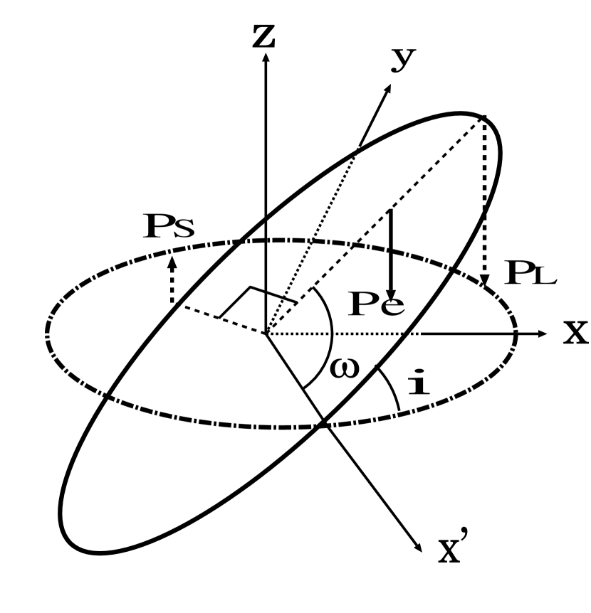
The mapping between the observed ellipse and the Keplerian orbit parameterized by the major axis and the ellipticity is specified by the inclination angle and the ascending node (See Fig. 1).
Given , , and , one can analytically determine the remaining parameters , , and in order as (Asada et al. 2004)
| (43) | |||
| (44) | |||
| (45) | |||
| (46) |
where
| (47) | |||
| (48) | |||
| (49) |
4 Numerical test
In this section, we verify the present formula by numerical computations for various values of the orbital parameters. In order to make a verification, we assume random errors in measurements of positions of the star and show that the orbital parameters are reconstructed: First, we assume a Keplerian orbit specified by and and a projection defined by and . We prepare twenty seven sets of the parameters as , , deg. and deg.
For each test, we pick up twelve points in the original Kepler orbit by assuming the same time interval between neighboring points for simplicity. Next, for assumed and , we estimate the projected locations of the twelve points in the apparent ellipse plane. We add random errors to each point in order to imitate a “measured position” with observational errors (See Fig. 2). In order to produce such a simulated data, we assume that the absolute standard deviation of the random error in the position measurement is 0.001 in the units of . We apply our formula to the simulated data in order to determine the orbital elements, and make a comparison between the assumed value and the retrieved one. Table 1 shows a good agreement between them.
For each parameter set, we perform a hundred of numerical runs for a statistical treatment. We define an error as the absolute standard deviation as , , and , where the prime denotes values retrieved by using the present formula and the square bracket denotes a mean over each set. In Table 1, asterisk () indicates that the formula does not always give a real value but a complex one. The case of complex numbers occurs because a large error in measurements of the positions in the apparent ellipse plane causes an anomaly in the apparent motion such as an apparent clockwise motion even if a true one is anti-clockwise.
It is worthwhile to make a comment on Table 1: In the case of no inclination as , the ascending node does not exist, so that an error in retrieving can be apparently quite large, though it is harmless.
5 Conclusion
In this paper, as a simplified method to determine a binary orbit, we extend the solution considering observational data. We expect that the present formula will be used for orbit determinations by some planned astrometric space missions such as SIM111http://sim.jpl.nasa.gov/ (Shao 2004), GAIA222http://astro.estec.esa.nl/GAIA/ (Mignard 2004, Perryman 2004) and JASMINE333http://www.jasmine-galaxy.org/ (Gouda et al. 2004), which will observe with the accuracy of possibly a few micro arcseconds a number of binaries whose components are a visible star and a companion ranging from a black hole to an extra-solar planet. Our numerical computations correspond to a case that by these missions we observe a binary system at a distance of 1 kpc from us, where the semimajor axis of the primary’s orbit is around 1AU.
References
- (1) Aitken R. G., 1964 The Binary Stars (NY: Dover)
- (2) Asada H., Akasaka T., Kasai M., 2004, PASJ., 56, L35
- (3) Asada H., 2006, Celest. Mech. in press (astro-ph/0609769)
- (4) Benedict G. F. et al., 2002, ApJ., 581, L115
- (5) Beutler G., 2004 Methods of Celestial Mechanics (Berlin: Springer)
- (6) Catovic Z., Olevic D., 1992 in IAU Colloquim 135, ASP Conference Series Vol. 32 (eds McAlister H. A., Hartkopf W. I., ) 217-219 (San Francisco, Astronomical Society of the Pacific).
- (7) Danby J. M. A., 1988 Fundamentals of Celestial Mechanics (VA: William-Bell)
- (8) Eichhorn H. K., Xu Y., 1990, ApJ., 358, 575
- (9) Goldstein H., 1980 Classical Mechanics (MA: Addison-Wesley)
- (10) Gouda N. et al., ‘Japan Astrometry Satellite Mission for Infrared Exploration (JASMINE)’, Proc. The Three-Dimensional Universe with Gaia, 4-7 October 2004, Paris (Netherlands: ESA Publications)
- (11) Mignard F., ‘Overall Science Goals of the Gaia Mission’, Proc. The Three-Dimensional Universe with Gaia, 4-7 October 2004, Paris (Netherlands: ESA Publications)
- (12) Miyoshi M. et al., 1995, Nature, 373, 127
- (13) Murray C. D., Dermott S. F., 1999 Solar System Dynamics (Cambridge: Cambridge Univ. Press)
- (14) Olevic D., Cvetkovic Z., 2004, A&A, 415, 259
- (15) Perryman M. A. C., ‘Overview of the Gaia Mission’, Proc. The Three-Dimensional Universe with Gaia, 4-7 October 2004, Paris (Netherlands: ESA Publications)
- (16) Roy A. E., 1988 Orbital Motion (Bristol: Institute of Physics Publishing)
- (17) Shao M., 2004, ’Science Overview and Status of the SIM Project’, SPIE 5491-36
- (18) Weaver H. A. et al., 2006, Nature, 439, 943

| [deg.] | [deg.] | |||
|---|---|---|---|---|
| 1-0.1- 0- 0 | 0.00113 | 0.00271 | 3.27 | 50.9 |
| 1-0.1- 0-30 | 0.00106 | 0.00258 | 3.16 | 24.7 |
| 1-0.1- 0-60 | * | * | * | * |
| 1-0.1-30- 0 | 0.000866 | 0.00305 | 0.116 | 1.34 |
| 1-0.1-30-30 | 0.00110 | 0.00296 | 0.154 | 1.30 |
| 1-0.1-30-60 | 0.00110 | 0.00343 | 0.122 | 1.04 |
| 1-0.1-60- 0 | 0.00112 | 0.00450 | 0.0574 | 2.08 |
| 1-0.1-60-30 | 0.00193 | 0.00544 | 0.0951 | 2.20 |
| 1-0.1-60-60 | 0.00141 | 0.00501 | 0.0605 | 1.90 |
| 1-0.3- 0- 0 | 0.00180 | 0.00497 | 4.29 | 47.5 |
| 1-0.3- 0-30 | 0.00166 | 0.00516 | 4.29 | 27.8 |
| 1-0.3- 0-60 | 0.00193 | 0.00555 | 4.52 | 28.4 |
| 1-0.3-30- 0 | 0.000933 | 0.00518 | 0.224 | 0.943 |
| 1-0.3-30-30 | 0.00175 | 0.00542 | 0.317 | 0.719 |
| 1-0.3-30-60 | 0.00142 | 0.00597 | 0.164 | 0.449 |
| 1-0.3-60- 0 | 0.00157 | 0.00884 | 0.122 | 1.17 |
| 1-0.3-60-30 | 0.00238 | 0.00856 | 0.150 | 0.832 |
| 1-0.3-60-60 | 0.00227 | 0.00797 | 0.0888 | 0.715 |
| 1-0.6- 0- 0 | 0.0105 | 0.0137 | 9.16 | 54.6 |
| 1-0.6- 0-30 | 0.00977 | 0.0147 | 9.24 | 34.8 |
| 1-0.6- 0-60 | 0.0131 | 0.0150 | 9.48 | 33.3 |
| 1-0.6-30- 0 | 0.00240 | 0.0168 | 1.67 | 2.37 |
| 1-0.6-30-30 | 0.00374 | 0.0172 | 1.32 | 2.48 |
| 1-0.6-30-60 | 0.00953 | 0.0150 | 0.623 | 2.54 |
| 1-0.6-60- 0 | 0.00400 | 0.0279 | 0.919 | 1.68 |
| 1-0.6-60-30 | 0.00614 | 0.0287 | 0.765 | 0.966 |
| 1-0.6-60-60 | 0.0117 | 0.0191 | 0.256 | 0.586 |